Abstract
We provide a stochastic extension of the Baez–Fritz–Leinster characterization of the Shannon information loss associated with a measure-preserving function. This recovers the conditional entropy and a closely related information-theoretic measure that we call conditional information loss. Although not functorial, these information measures are semi-functorial, a concept we introduce that is definable in any Markov category. We also introduce the notion of an entropic Bayes’ rule for information measures, and we provide a characterization of conditional entropy in terms of this rule.
Keywords:
Bayes; conditional probability; disintegration; entropy; error correction; functor; information theory; Markov category; stochastic map; synthetic probability MSC:
Primary 94A17; Secondary 18A05; 62F15
1. Introduction
The information loss associated with a measure-preserving function between finite probability spaces is given by the Shannon entropy difference
where is the Shannon entropy of p (and similarly for q). In [1], Baez, Fritz, and Leinster proved that the information loss satisfies, and is uniquely characterized up to a non-negative multiplicative factor by, the following conditions:
- 0.
- Positivity: for all . This says that the information loss associated with a deterministic process is always non-negative.
- 1.
- Functoriality: for every composable pair of measure-preserving maps. This says that the information loss of two successive processes is the sum of the information losses associated with each process.
- 2.
- Convex Linearity: for all . This says that the information loss associated with tossing a (possibly unfair) coin in deciding amongst two processes is the associated weighted sum of their information losses.
- 3.
- Continuity: is a continuous function of f. This says that the information loss does not change much under small perturbations (i.e., is robust with respect to errors).
As measure-preserving functions may be viewed as deterministic stochastic maps, it is natural to ask whether there exist extensions of the Baez–Fritz–Leinster (BFL) characterization of information loss to maps that are inherently random (i.e., stochastic) in nature. In particular, what information-theoretic quantity captures such an information loss in this larger category?
This question is answered in the present work. Namely, we extend the BFL characterization theorem, which is valid on deterministic maps, to the larger category of stochastic maps. In doing so, we also find a characterization of the conditional entropy. Although the resulting extension is not functorial on the larger category of stochastic maps, we formalize a weakening of functoriality that restricts to functoriality on deterministic maps. This weaker notion of functoriality is definable in any Markov category [2,3], and it provides a key axiom in our characterization.
To explain how we arrive at our characterization, let us first recall the definition of stochastic maps between finite probability spaces, for which the measure-preserving functions are a special case. A stochastic map associates with every a probability distribution on Y such that , where is the distribution evaluated at . In terms of information flow, the space may be thought of as a probability distribution on the set of inputs for a communication channel described by the stochastic matrix , while is then thought of as the induced distribution on the set of outputs of the channel.
Extending the information loss functor by assigning to any stochastic map would indeed result in an assignment that satisfies conditions 1–3 listed above. However, it would no longer be positive and the interpretation as an information loss would be gone. Furthermore, no additional information about the stochasticity of the map f would be used in determining this assignment. In order to guarantee positivity, an additional term, depending on the stochasticity of f, is needed. This term is provided by the conditional entropy of and is given by the the non-negative real number
where is the Shannon entropy of the distribution on Y (in the case that and are probability spaces associated with the alphabets of random variables and , then coincides with conditional entropy [4]). If is in fact deterministic, i.e., if is a point-mass distribution for all , then for all . As such, is a measure of the uncertainty (or randomness) of the outputs of f averaged over the prior distribution p on the set X of its inputs. Indeed, is maximized precisely when is the uniform distribution on Y for all .
Therefore, given a stochastic map , we call
the conditional information loss of (the same letter K is used here because it agrees with the Shannon entropy difference when f is deterministic). As whenever f is deterministic, the conditional information loss restricts to the category of measure preserving functions as the information loss functor of Baez, Fritz, and Leinster, while also satisfying conditions 0, 2, and 3 (i.e., positivity, convex linearity, and continuity) on the larger category of stochastic maps. However, conditional information loss is not functorial in general, and while this may seem like a defect at first glance, we prove that there is no extension of the information loss functor that remains functorial on the larger category of stochastic maps if the positivity axiom is to be preserved, thus retaining an interpretation as information loss. In spite of this, conditional information loss does satisfy a weakened form of functoriality, which we briefly describe now.
A pair of composable stochastic maps is a.e. coalescable if and only if for every pair of elements and for which and , there exists a unique such that and . Intuitively, this says that the information about the intermediate step can be recovered given knowledge about the input and output. In particular, if f is deterministic, then the pair is a.e. colescable (for obvious reasons, since knowing x alone is enough to determine the intermediate value). However, there are other many situations where a pair could be a.e. coalescable and the maps need not be deterministic. With this definition in place (which we also generalize to the setting of arbitrary Markov categories), we replace functoriality with the following weaker condition.
- 1🟉.
- Semi-functoriality: for every a.e. coalescable pair of stochastic maps. This says that the conditional information loss of two successive processes is the sum of the conditional information losses associated with each process provided that the information in the intermediate step can always be recovered.
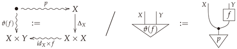
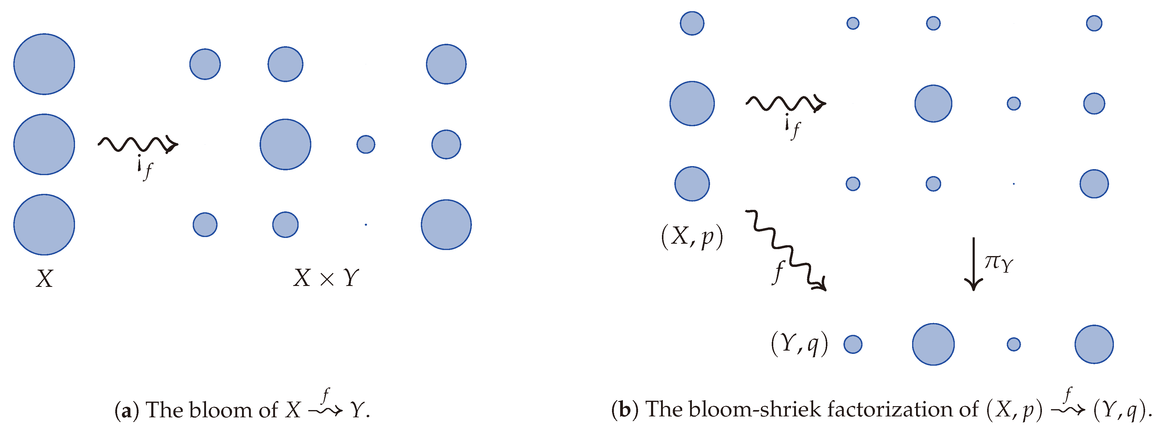
Replacing functoriality with semi-functoriality is not enough to characterize the conditional information loss. However, it comes quite close, as only one more axiom is needed. Assuming positivity, semi-functoriality, convex linearity, and continuity, there are several equivalent axioms that may be stipulated to characterize the conditional information loss. To explain the first option, we introduce a convenient factorization of every stochastic map . The bloom-shriek factorization of f is given by the decomposition , where is the bloom of f whose value at is the probability measure on given by sending to , where is the Kronecker delta. In other words, records each of the probability measures on a copy of Y indexed by . A visualization of the bloom of f is given in Figure 1a. When one is given the additional data of probability measures p and q on X and Y, respectively, then Figure 1b illustrates the bloom-shriek factorization of f. From this point of view, keeps track of the information encoded in both p and f, while the projection map forgets, or loses, some of this information.
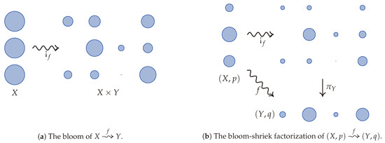
Figure 1.
A visualization of bloom and the bloom-shriek factorization via water droplets as inspired by Gromov [5]. The bloom of f splits each water droplet of volume 1 (an element of X) into several water droplets whose total volume equates to 1. If X has a probability p on it, then the initial volume of that water droplet is scaled by this probability. The stochastic map therefore splits the water droplet using this scale.
With this in mind, our final axiom to characterize the conditional information loss is
- 4(a).
- Reduction: , where is the bloom-shriek factorization of f. This says that the conditional information loss of f equals the information loss of the projection using the associated joint distribution on .
Note that this axiom describes how K is determined by its action on an associated class of deterministic morphisms. These slightly modified axioms, namely, semi-functoriality, convex linearity, continuity, and reduction, characterize the conditional information loss and therefore extend Baez, Fritz, and Leinster’s characterization of information loss. A much simpler axiom that may be invoked in place of the reduction axiom which also characterizes conditional information loss is the following.
- 4(b).
- Blooming: , where is the unique map from a one point probability space to . This says that if a process begins with no prior information, then there is no information to be lost in the process.
The conditional entropy itself can be extracted from the conditional information loss by a process known as Bayesian inversion, which we now briefly recall. Given a stochastic map , there exists a stochastic map such that for all and (the stochastic map is the almost everywhere unique conditional probability so that Bayes’ rule holds). Such a map is called a Bayesian inverse of f. The Bayesian inverse can be visualized using the bloom-shriek factorization because it itself has a bloom-shriek factorization . This is obtained by finding the stochastic maps in the opposite direction of the arrows so that they reproduce the appropriate volumes of the water droplets.
Given this perspective on Bayesian inversion, we prove that the conditional entropy of equals the conditional information loss of its Bayesian inverse . Moreover, since the conditional information loss of is just the information loss of , this indicates how the conditional entropy and conditional information losses are the ordinary information losses associated with the two projections and in Figure 1b. This duality also provides an interesting perspective on conditional entropy and its characterization. Indeed, using Bayesian inversion, we also characterize the conditional entropy as the unique assignment F sending measure-preserving stochastic maps between finite probability spaces to real numbers satisfying conditions 0, , 2, and 3 above, but with a new axiom that reads as follows.
- 4(c).
- Entropic Bayes’ Rule: for all . This is an information theoretic analogue of Bayes’ rule, which reads for all and , or in more traditional probabilistic notation
In other words, we obtain a Bayesian characterization of the conditional entropy. This provides an entropic and information-theoretic description of Bayes’ rule from the Markov category perspective, in a way that we interpret as answering an open question of Fritz [6].
2. Categories of Stochastic Maps
In the first few sections, we define all the concepts involved in proving that the conditional information loss satisfies the properties that we will later prove characterize it. This section introduces the domain category and its convex structure.
Definition 1.
Let X and Y be finite sets. Astochastic map associates a probability measure to every . If is such that is a point-mass distribution for every , then f is said to bedeterministic.
Notation 1.
Given a stochastic map (also written as ), the value will be denoted by . As there exists a canonical bijection between deterministic maps of the form and functions , deterministic maps from X to Y will be denoted by the functional notation .
Definition 2.
A stochastic map of the form from a single element set to a finite set X is a single probability measure on X. Its unique value at x will be denoted by for all . The set will be referred to as thenullspaceof p.
Definition 3.
LetFinStochbe the category of stochastic maps between finite sets. Given a finite set X, the identity map of X inFinStochcorresponds to the identity function . Second, given stochastic maps and , the composite is given by the Chapmann–Kolmogorov equation
Definition 4.
Let X be a finite set. Thecopyof X is the diagonal embedding , and thediscardof X is the unique map from X to the terminal object • inFinStoch, which will be denoted by . If Y is another finite set, theswap mapis the map given by . Given morphisms and inFinStoch, theproductof f and g is the stochastic map given by
The product of stochastic maps endows FinStoch with the structure of a monoidal category. Together with the copy, discard, and swap maps, FinStoch is a Markov category [2,3].
Definition 5.
Let (this stands for “finiteprobabilities andstochastic maps”) be the co-slice category , i.e., the category whose objects are pairs consisting of a finite set X equipped with a probability measure p, and a morphism from to is a stochastic map such that for all . The subcategory of deterministic maps in will then be denoted by (which stands for “finiteprobabilities anddeterministic maps”). A pair of morphisms in is said to be acomposable pairiff exists.
Note that the category was called in [1].
Remark 1.
Though it is often the case that we will denote a morphism in simply by f, such notation is potentially ambiguous, as the morphism is distinct from the morphsim whenever . As such, we will only employ the shorthand of denoting a morphism in by its underlying stochastic map whenever the source and target of the morphism are clear from the context.
Lemma 1.
The object given by a single element set equipped with the unique probability measure is a zero object (i.e., terminal and initial) in .
Definition 6.
Given an object in , theshriekandbloomof p are the unique maps to and from respectively, which will be denoted and (the former is deterministic, while the latter is stochastic). The underlying stochastic maps associated with and are and , respectively.
Example 1.
Since is a zero object, given any two objects and , there exists at least one morphism , namely the composite .
Definition 7.
Let be a morphism in . Thejoint distributionassociated with f is the probability measure given by .
It is possible to take convex combinations of both objects and morphisms in , and such assignments will play a role in our characterization of conditional entropy.
Definition 8.
Let be a probability measure and let be a collection of objects in indexed by X. The p-weighted convex sum is defined to be the set equipped with the probability measure given by
In addition, if is a collection of morphisms in indexed by X, the p-weighted convex sum is given by
3. The Baez–Fritz–Leinster Characterization of Information Loss
In [1], Baez, Fritz, and Leinster (BFL) characterized the Shannon entropy difference associated with measure-preserving functions between finite probability spaces as the only non-vanishing, continuous, convex linear functor from to the non-negative reals (up to a multiplicative constant). It is then natural to ask whether there exist either extensions or analogues of their result by including non-deterministic morphisms from the larger category . Before delving deeper into such inquiry, we first recall in detail the characterization theorem of BFL.
Definition 9.
Let be the convex category consisting of a single object and whose set of morphisms is . The composition in is given by addition. Convex combinations of morphisms are given by ordinary convex combinations of numbers. The subcategory of non-negative reals will be denoted .
In the rest of the paper, we will not necessarily assume that assignments from one category to another are functors. Nevertheless, we do assume they form (class) functions (see ([7], Section I.7) for more details). Furthermore, we assume that they respect or reflect source and targets in the following sense. If and are two categories, all functions are either covariant or contravariant in the sense that for any morphism in , is a morphism from to or from to , respectively. These are the only types of functions between categories we will consider in this work. As such, we therefore abuse terminology and use the term functions for such assignments throughout. If M is a commutative monoid and denotes its one object category, then every covariant function is also contravariant and vice-versa.
We now define a notion of continuity for functions of the form .
Definition 10.
A sequence of morphisms in convergesto a morphism if and only if the following two conditions hold.
- (a)
- There exists an for which and for all .
- (b)
- The following limits hold: and (note that these limits necessarily imply ).
A function iscontinuousif and only if whenever is a sequence in converging to f.
Remark 2.
In the subcategory , since the topology of the collection of functions from a finite set X to another finite set Y is discrete, one can equivalently assume that a sequence as in Definition 10, but this time with all deterministic, converges to if and only if the following two conditions hold.
- (a)
- There exists an for which for all .
- (b)
- For , one has .
In this way, our definition of convergence agrees with the definition of convergence of BFL on the subcategory [1].
Definition 11.
A function is said to beconvex linearif and only if for all objects in ,
for all collections in .
Definition 12.
A function is said to befunctorialif and only if it is in fact a functor, i.e., if and only if for every composable pair in .
Definition 13.
Let be a probability measure. TheShannon entropyof p is given by
When considering any entropic quantity, we will always adhere to the convention that .
Definition 14.
Given a map in , the Shannon entropy difference will be referred to as theinformation lossof f. Information loss defines a functor , henceforth referred to as theinformation loss functoron .
Theorem 1
(Baez–Fritz–Leinster [1]). Suppose is a function which satisfies the following conditions.
- 1.
- F is functorial.
- 2.
- F is convex linear.
- 3.
- F is continuous.
Then F is a non-negative multiple of information loss. Conversely, the information loss functor is non-negative and satisfies conditions 1–3.
In light of Theorem 1, it is natural to question whether or not there exists a functor that restricts to as the information loss functor. It turns out that no such non-vanishing functor exists, as we prove in the following proposition.
Proposition 1.
If is a functor, then for all morphisms f in .
Proof.
Let be a morphism in . Since F is a functor,
Let be any morphism in (which necessarily exists by Example 1, for instance). Then a similar calculation yields
Hence, . □
4. Extending the Information Loss Functor
Proposition 1 shows it is not possible to extend the information loss functor to a functor on . Nevertheless, in this section, we define a non-vanishing function that restricts to the information loss functor on , which we refer to as conditional information loss. While K is not functorial, we show that it satisfies many important properties such as continuity, convex linearity, and invariance with respect to compositions with isomorphisms. Furthermore, in Section 5 we show K is functorial on a restricted class of composable pairs of morphisms (cf. Definition 18), which are definable in any Markov category. At the end of this section we characterize conditional information loss as the unique extension of the information loss functor satisfying the reduction axiom 4(a) as stated in the introduction. In Section 8, we prove an intrinsic characterization theorem for K without reference to the deterministic subcategory inside . Appendix A provides an interpretation of the vanishing of conditional information loss in terms of correctable codes.
Definition 15.
Theconditional information lossof a morphism in is the real number given by
where
is theconditional entropyof .
Proposition 2.
The function , uniquely determined on morphisms by sending to , satisfies the following conditions.
- (i)
- .
- (ii)
- K restricted to agrees with the information loss functor (cf. Definition 14).
- (iii)
- K is convex linear.
- (iv)
- K is continuous.
- (v)
- Given , then , where is the projection and is the joint distribution (cf. Definition 7).
Lemma 2.
Let be a morphism in . Then
Proof of Lemma 2.
Applying K to f yields
Proof of Proposition 2.
- (i)
- The non-negativity of K follows from Lemma 2 and the equality .
- (ii)
- This follows from the fact that for all deterministic f.
- (iii)
- Let be a probability measure, and let be a collection of morphisms in indexed by X. Then the p-weighted convex sum is a morphism in of the form , where , , , , and . Thenwhich shows that K is convex linear.
- (iv)
- Let be a sequence (indexed by ) of probability-preserving stochastic maps such that and for large enough n, and where and . Thenwhere the last equality follows from the fact that the limit and sum (which is finite) can be interchanged and all expressions are continuous on .
- (v)
- This follows fromand the fact that . □
Remark 3.
Since conditional entropy vanishes for deterministic morphisms, conditional information loss restricts to as the information loss functor. It is important to note that if the term was not included in the expression for , then the inequality would fail in general. When f is deterministic, Baez, Fritz, and Leinster proved . However, when f is stochastic, the inequality does not hold in general. This has to do with the fact that stochastic maps may increase entropy, whereas deterministic maps always decrease it(while this claim holds in the classical setting as stated, it no longer holds for quantum systems [8]). As such, the term is needed to retain non-negativity as one attempts to extend BFL’s functor K on to a function on .
Item (v) of Proposition 2 says that the conditional information loss of a map in is the information loss of the deterministic map in , so that conditional information loss of a morphism in may always be reduced to the information loss of a deterministic map in naturally associated with it having the same target. This motivates the following definition.
Definition 16.
A function isreductiveif and only if for every morphism in (cf. Proposition 2 item (v) for notation).
Proposition 3
(Reductive characterization of conditional information loss). Let be a function satisfying the following conditions.
- (i)
- F restricted to is functorial, convex linear, and continuous.
- (ii)
- F is reductive.
Then F is a non-negative multiple of conditional information loss. Conversely, conditional information loss satisfies conditions (i) and (ii).
Proof.
This follows immediately from Theorem 1 and item (v) of Proposition 2. □
In what follows, we will characterize conditional information loss without any explicit reference to the subcatgeory or the information loss functor of Baez, Fritz, and Leinster. To do this, we first need to develop some machinery.
5. Coalescable Morphisms and Semi-Functoriality
While conditional information loss is not functorial on , we know it acts functorially on deterministic maps. As such, it is natural to ask for which pairs of composable stochastic maps does the conditional information loss act functorially. In this section, we answer this question, and then we use our result to define a property of functions that is a weakening of functoriality, and which we refer to as semi-functoriality. Our definitions are valid in any Markov category (cf. Appendix B).
Definition 17.
A deterministic map is said to be amediatorfor the composable pair in if and only if
If in fact Equation (1) holds for all , then h is said to be astrong mediatorfor the composable pair inFinStoch.
Remark 4.
Mediators do not exist for general composable pairs, as one can see by considering any composable pair such that (cf. Definitions 7 and 13).
Proposition 4.
Let be a composable pair of morphisms in . Then the following statements are equivalent.
- (a)
- For every and , there exists at most one such that .
- (b)
- The pair admits a mediator .
- (c)
- There exists a function such that
Proof.
((a)⇒(b)) For every for which such a y exists, set . If no such y exists or if , set to be anything. Then h is a mediator for .
((b)⇒(c)) Let h be a mediator for . Since (2) holds automatically for , suppose , in which case (2) is equivalent to for all . This follows from Equation (1) and the fact that h is a function.
((c)⇒(a)) Let and suppose . If h is the mediator, then . But since for all , there is only one non-vanishing term in this sum, and it is precisely . □
Theorem 2
(Functoriality of Conditional Entropy). Let be a composable pair of morphisms in . Then
holds if and only if there exists a mediator for .
We first prove two lemmas.
Lemma 3.
Let be a pair of composable morphisms. Then
In particular, if and only if .
Proof of Lemma 3.
On components, . Hence,
Note that this equality still holds if or as each step in this calculation accounted for such possibilities. □
Lemma 4.
Let be a pair of composable morphisms in . Then
Note that the order of the sums matters in this expression and also note that it is always well-defined since implies .
Proof of Lemma 4.
For convenience, temporarily set . Then
which proves the claim due to the definition of the composition of stochastic maps. □
Proof of Theorem 2.
Temporarily set . In addition, note that the set of all and can be given a more explicit description in terms of the joint distribution associated with the composite and prior p, namely . Then,
(⇒) Suppose , which is equivalent to Equation (3) by Lemma 3. Then since each term in the sum from Lemma 4 is non-negative,
Hence, fix such an . The expression here vanishes if and only if
Hence, for every and , there exists a unique such that . But by (5), this means that for every , there exists a unique such that . This defines a function which can be extended in an s-a.e. unique manner to a function
We now show the function h is in fact a mediator for the composable pair . The equality clearly holds if since both sides vanish. Hence, suppose that . Given , the left-hand-side of (2) is given by
by Equation (6). Similarly, if and , then for all because otherwise would be nonzero. If instead , then and for all by (6). Therefore, (2) holds.
(⇐) Conversely, suppose a mediator h exists and let be the stochastic map given on components by Then
as desired. □
Corollary 1
(Functoriality of Conditional Information Loss). Let be a composable pair of morphisms in . Then if and only if there exists a mediator for the pair .
Proof.
Since the Shannon entropy difference is always functorial, the conditional information loss is functorial on a pair of morphisms if and only if the conditional entropy is functorial on that pair. Theorem 2 then completes the proof. □
Example 2.
In the notation of Theorem 2, suppose that f isa.e. deterministic, which means for all for some function f (abusive notation is used). In this case, the deviation from functoriality, (4), simplifies to
Therefore, if f is p-a.e. deterministic, . In this case, the mediator is given by .
Definition 18.
A pair of composable morphisms in is calleda.e. coalescableif and only if admits a mediator . Similarly, a pair of composable morphisms inFinStochis calledcoalescableiff admits a strong mediator .
Remark 5.
Example 2 showed that if is p-a.e. deterministic, then the pair is a.e. coalescable for any g. In particular, every pair of composable morphisms in is coalescable.
In light of Theorem 2 and Corollary 1, we make the following definition, which will serve as one of the axioms in our later characterizions of both conditional information loss and conditional entropy.
Definition 19.
A function is said to besemi-functorialiff for every a.e. coalescable pair in .
Example 3.
By Theorem 2 and Corollary 1, conditional information loss and conditional entropy are both semi-functorial.
Proposition 5.
Suppose is semi-functorial. Then the restriction of F to is functorial. In particular, if F is, in addition, convex linear, continuous, and reductive, then F is a non-negative multiple of conditional information loss.
Proof.
By Example 2, every pair of composable morphisms in is a.e. coalescable. Therefore, F is functorial on . The second claim then follows from Proposition 3. □
The following lemma will be used in later sections and serves to illustrate some examples of a.e. coalescable pairs.
Lemma 5.
Let be a triple of composable morphisms with e deterministic and g invertible. Then each of the following pairs are a.e. coalescable:
- (i)
- (ii)
- (iii)
- (iv)
Proof.
The proof that is coalescable was provided (in a stronger form) in Example 2. To see that is coalescable, note that since g is an isomorphism we have . Thus, is a mediator function for , thus is coalescable. The last two claims follow from the proofs of the first two claims. □
6. Bayesian Inversion
In this section, we recall the concepts of a.e. equivalence and Bayesian inversion phrased in a categorical manner [2,3,9], as they will play a significant role moving forward.
Definition 20.
Let and be two morphisms in with the same source and target. Then f and g are said toalmost everywhere equivalent(or p-a.e.equivalent) if and only if for every with . In such a case, the p-a.e. equivalence of f and g will be denoted .
Theorem 3
(Bayesian Inversion [2,9,10]). Let be a morphism in . Then there exists a morphism such that for all and . Furthermore, for any other morphism satisfying this condition, .
Definition 21.
The morphism appearing in Theorem 3 will be referred to as aBayesian inverseof . It follows that for all with .
Proposition 6.
Bayesian inversion satisfies the following properties.
- (i)
- Suppose and are p-a.e. equivalent, and let and be Bayesian inverses of f and g, respectively. Then .
- (ii)
- Given two morphisms and in , then f is a Bayesian inverse of g if and only if g is a Bayesian inverse of f.
- (iii)
- Let be a Bayesian inverse of , and let be the swap map (as in Definition 4). Then
- (iv)
- Let be a composable pair of morphisms in , and suppose and are Bayesian inverses of f and g respectively. Then is a composable pair, and is a Bayesian inverse of .
Proof.
These are immediate consequences of the categorical definition of a Bayesian inverse (see [3,10,11] for proofs). □
Definition 22.
A contravariant function is said to be aBayesian inversion functorif and only if acts as the identity on objects and is a Bayesian inverse of f for all morphisms f in .
This is mildly abusive terminology since functoriality only holds in the a.e. sense, as explained in the following remark.
Remark 6.
A Bayesian inversion functor exists. Given any , set to be given by for all with and for all with . Note that this does not define a functor. Indeed, if is a probability space with for some , then is the uniform measure on X instead of the Dirac delta measure concentrated on . In other words, . Similar issues of measure zero occur, indicating that for a composable pair of morphisms . Nevertheless, Bayesian inversion is a.e. functorial in the sense that and .
Corollary 2.
for any Bayesian inversion functor and every in .
Proposition 7.
Let be a Bayesian inversion functor on (as in Definition 22). Then isa.e. convex linearin the sense that
where and the other notation is as in Definition 8.
Proof.
First note that it is immediate that is convex linear on objects since Bayesian inversion acts as the identity on objects. Let be a probability measure, be a collection of morphisms in indexed by X, and suppose is a Bayesian inversion functor. Then for with , we have
Thus, is a.e. convex linear. □
Proposition 8.
Given in , and let and be Bayesian inverses of f and g respectively. Then is a.e. coalescable if and only if is a.e. coalescable.
Proof.
Since Bayesian inversion is a dagger functor on a.e. equivalence classes ([3], (Remark 13.10)), it suffices to prove one direction in this claim. Hence, suppose is a.e. coalescable and let h be a mediator function realizing this. Then is a mediator for because
A completely string-diagrammatic proof is provided in Appendix B. □
The following proposition is a reformulation of the conditional entropy identity in terms of Bayesian inversion.
Proposition 9.
Let be a morphism in , and suppose is a Bayesian inverse of f. Then
Proof.
This follows from the fact that both sides of (7) are equal to . □
Proposition 9 implies Bayesian inversion takes conditional entropy to conditional information loss and vice versa, which is formally stated as follows.
Corollary 3.
Let and be given by conditional information loss and conditional entropy, respectively, and let be a Bayesian inversion functor. Then, and .
Remark 7.
If is a deterministic morphism in , Baez, Fritz, and Leinster point out that the information loss of f is in fact the conditional entropy of x given y [1]. Here, we see this duality as a special case of Corollary 3 applied to deterministic morphisms.
7. Bloom-Shriek Factorization
We now introduce a simple, but surprisingly useful, factorization for every morphism in , and we use it to prove some essential lemmas for our characterization theorems for conditional information loss and conditional entropy, which appear in the following sections.
Definition 23.
Given a stochastic map , thebloom of fis the stochastic map given by the composite , and theshriek of fis the deterministic map given by the projection .
Proposition 10.
Let be a morphism in . Then the following statement hold.
- (i)
- The composite is equal to the identity .
- (ii)
- The morphism f equals the composite , where denotes any Bayesian inverse of f and is the swap map.
- (iii)
- The pair is coalescable.
Definition 24.
The decomposition in item (ii) Proposition 10 will be referred to as thebloom-shriek factorizationof f.
Proof of Propostion 10.
Element-wise proofs are left as exercises. Appendix B contains an abstract proof using string diagrams in Markov categories. □
The bloom of f can be expressed as a convex combination of simpler morphisms up to isomorphism. To describe this and its behavior under convex linear semi-functors, we introduce the notion of an invariant and examine some of its properties.
Definition 25.
A function is said to be aninvariantif and only if for every triple of composable morphisms such that e and g are isomorphisms, then .
Lemma 6.
If a function is semi-functorial, then F is an invariant.
Proof.
Consider a composable triple such that e and g are isomorphisms. Then
by Lemma 5. Secondly, since g and e are isomorphisms, and since the pairs and are coalescable, . But since (by semi-functoriality), this requires that for an isomorphism g since and . The same is true for . Hence, . □
Lemma 7.
Let be a morphism in , and suppose is semi-functorial and convex linear. Then the following statements hold.
- (i)
- (ii)
- (iii)
Proof.
For item (i), we have
For items (ii) and (iii), note that and can be expressed as composites of isomorphisms and certain convex combinations, namely
 Hence,
Proposition 11.
Suppose is semi-functorial and convex linear. If are two morphisms in such that , then .
Proof.
Suppose and are such that , and let and be Bayesian inverses for f and g. Then
as desired. □
8. An Intrinsic Characterization of Conditional Information Loss
Theorem 4.
Suppose is a function satisfying the following conditions.
- 1.
- F is semi-functorial.
- 2.
- F is convex linear.
- 3.
- F is continuous.
- 4.
- for every probability distribution .
Then F is a non-negative multiple of conditional information loss. Conversely, conditional information loss satisfies conditions 1–4.
Proof.
Suppose F satisfies conditions 1–4, let be an arbitrary morphism in , and let be the swap map, so that . Then
Thus, F is reductive (see Definition 16) and Proposition 5 applies. □
Remark 8.
Under the assumption that is semi-functorial and convex linear, one may show F satisfies condition 4 in Theorem 4 if and only if F is reductive (see Definition 16 and Proposition 5). While the reductive axiom specifies how the semi-functor acts on all morphisms in , condition 4 in Theorem 4 only specifies how it acts on morphisms from the initial object. This gives not just a simple mathematical criterion, but one with a simple intuitive interpretation as well. Namely, condition 4 says that if a process begins with no prior information, then there is no information to be lost in the process.
We now use Theorem 4 and Bayesian inversion to prove a statement dual to Theorem 4.
Theorem 5.
Suppose is a function satisfying the following conditions.
- 1.
- F is semi-functorial.
- 2.
- F is convex linear.
- 3.
- F is continuous.
- 4.
- for every probability distribution .
Then F is a non-negative multiple of conditional entropy. Conversely, conditional entropy satisfies conditions 1–4.
Before giving a proof, we introduce some terminology and prove a few lemmas. We also would like to point out that condition 4 may be given an operational interpretation as follows: if a communication channel has a constant output, then it has no conditional entropy.
Definition 26.
Let be a function and let be a Bayesian inversion functor. Then will be referred to as aBayesian reflectionof F.
Remark 9.
By Proposition 11, if is a convex linear semi-functor, then a Bayesian reflection is independent of the choice of a Bayesian inversion functor, and as such, is necessarily unique.
Lemma 8.
Let be a morphism in , suppose is a convex linear semi-functor, and let be a Bayesian inverse of f. Then .
Proof of Lemma 8.
Let be a Bayesian inversion functor, so that . Then where the last equality follows from Proposition 11. □
Lemma 9.
Let be a Bayesian inversion functor and let be a sequence of morphisms in converging to . Then .
Proof of Lemma 9.
Set . For all with , we have
Lemma 10.
Suppose is a function satisfying conditions 1–4 of Theorem 5. Then the Bayesian reflection is a non-negative multiple of conditional information loss.
Proof of Lemma 10.
We show satisfies conditions 1–4 of Theorem 4. Throughout the proof, let denote a Bayesian inversion functor, so that .
Semi-functoriality: Suppose is an a.e. coalescable pair of composable morphisms in . Then
Thus, is semi-functorial.
Convex Linearity: Given any probability space and a family of morphisms in indexed by X,
Thus, is convex linear.
Continuity: This follows from Lemma 9 and Proposition 11.
for every probability distribution : This follows from Lemma 8, since is the unique Bayesian inverse of . □
Proof of Theorem 5.
Suppose is a function satisfying conditions 1–4 of Theorem 5, and let be a Bayesian inversion functor. Since F is semi-functorial and convex linear it follows from Proposition 11 that , and by Lemma 10 it follows that for some non-negative constant . We then have . Thus, F is a non-negative multiple of conditional entropy. □
9. A Bayesian Characterization of Conditional Entropy
We now prove a reformulation of Theorem 5, where condition 4 is replaced by a condition that we view as an ‘entropic Bayes’ rule’.
Definition 27.
A function satisfies anentropic Bayes’ ruleif and only if
for every morphism in and any Bayesian inverse of f.
Remark 10.
The entropic Bayes’ rule is an abstraction of the conditional entropy identity 7.
Theorem 6
(A Bayesian characterization of conditional entropy). Suppose is a function satisfying the following conditions.
- 1.
- F is semi-functorial.
- 2.
- F is convex linear.
- 3.
- F is continuous.
- 4.
- F satisfies an entropic Bayes’ rule.
Then F is a non-negative multiple of conditional entropy. Conversely, conditional entropy satisfies conditions 1–4.
Proof.
By Theorem 5, it suffices to show for every object in . For this, first note that , where is the point-mass distribution on a single point. Since F is semi-functorial and is coalescable, we have , which implies . Applying the entropic Bayes’ rule from Definition 27 to the morphism yields
as desired. □
Remark 11.
In ([6], slide 21), Fritz asked if there is a Markov category for information theory explaining the analogy between Bayes’ rule and the conditional entropy identity . In light of our work, we feel we have an adequate categorical explanation for this analogy, which we now explain.
Let be an arbitrary morphism in , and suppose is semi-functorial. Then the commutative diagram (cf. Definition A4)
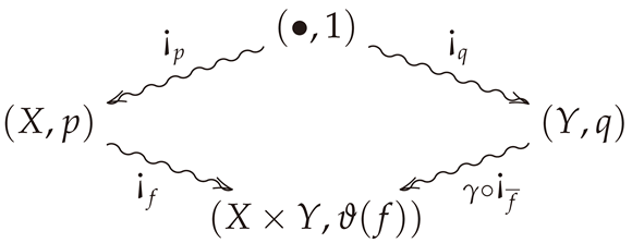 is a coalescable square (where γ is the swap map), i.e., and are both coalescable. The semi-functoriality of F then implies the identity . Now suppose—as in the case of conditional entropy—that F satisfies the further condition that . Then commutivity of (9) and this are equivalent to the following two respective equations:
In the case that , where H is the conditional entropy, we have for every object in (where is the Shannon entropy). Thus, the entropic Bayes’ rule becomes , which is the classical identity for conditional entropy.
is a coalescable square (where γ is the swap map), i.e., and are both coalescable. The semi-functoriality of F then implies the identity . Now suppose—as in the case of conditional entropy—that F satisfies the further condition that . Then commutivity of (9) and this are equivalent to the following two respective equations:
In the case that , where H is the conditional entropy, we have for every object in (where is the Shannon entropy). Thus, the entropic Bayes’ rule becomes , which is the classical identity for conditional entropy.
10. Concluding Remarks
In this paper, we have provided novel characterizations of conditional entropy and the information loss of a probability-preserving stochastic map. The constructions we introduced to prove our main results are general enough to be applicable in the recent framework of synthetic probability [3]. By weakening functoriality and finding the appropriate substitute that we call semi-functoriality, we have shown how certain aspects of quantitative information theory can be done in this categorical framework. In particular, we have illustrated how Bayes’ rule can be formulated entropically and used as an axiom in characterizing conditional entropy.
Immediate questions from our work arise, such as the extendibility of conditional entropy to other Markov categories or even quantum Markov categories [10]. Work in this direction might offer a systematic approach towards conditional entropy in quantum mechanics. It would also be interesting to see what other quantitative features of information theory can be described from such a perspective, or if new ones will emerge.
Author Contributions
Both authors contributed equally to this manuscript. Both authors have read and agreed to the published version of the manuscript.
Funding
This research has received funding from the European Research Council (ERC) under the European Union’s Horizon 2020 research and innovation program (QUASIFT grant agreement 677368).
Institutional Review Board Statement
Not applicable.
Informed Consent Statement
Not applicable.
Data Availability Statement
Not applicable.
Acknowledgments
We thank Tobias Fritz, Azeem ul Hassan, Francois Jacopin, Jiaxin Qiao, and Alex Atsushi Takeda for discussions.
Conflicts of Interest
The authors declare no conflict of interest.
Appendix A. Correctable Codes and Conditional Information Loss
In this appendix, we prove that the conditional information loss of a morphism in vanishes if and only if f is a disintegration, or equivalently, if and only if f is correctable (cf. Remark A1). Briefly, a disintegration is a particular kind of Bayesian inverse that we define momentarily. This provides an additional interpretation of the conditional information loss, namely as a deviation from correctability.
Definition A1.
Let be a morphism in . Then is said to be adisintegrationof g (or for clarity) if and only if .
Lemma A1.
If f is a disintegration of g, then g is q-a.e. deterministic and f is a Bayesian inverse of g. Conversely, if g is q-a.e. deterministic, then every Bayesian inverse of g is a disintegration of g.
Proof.
This is proved in a more abstract setting in ([10], Section 8). □
Theorem A1.
Let be a morphism in . Then if and only if there exists a map such that f is a disintegration of g.
Proof.
The theorem will be proved by showing the equivalent statement ‘ if and only if is q-a.e. deterministic for some Bayesian inverse of f.’ We therefore first justify this as being equivalent to the claim.
First, holds if and only if for some (and hence any) Bayesian inverse of f by Corollary 3 and Lemma 8. Second, the statement ‘there exists a g such that f is a disintegration of g’ holds if and only if ‘there exists a g such that f is a Bayesian inverse of g and g is q-a.e. deterministic’ by Lemma A1. However, since Bayesian inverses always exist (Theorem 3), and because Bayesian inversion is symmetric (item (ii) in Proposition 6), this latter statement is equivalent to ‘there exists a q-a.e. deterministic Bayesian inverse g of f.’
Hence, suppose f has a q-a.e. deterministic Bayesian inverse g. Then
since the entropy of vanishes because it is -valued for all .
Conversely, suppose for some Bayesian inverse of f. Then is a sum of non-negative numbers that vanishes. Hence, for all . But since the entropy of a probability measure on a finite set vanishes if and only if the probability measure is -valued, is -valued for all . Hence, is q-a.e. deterministic. □
Remark A1
(Vanishing of Conditional Information Loss in Terms of Correctable Codes). The vanishing of the conditional information loss is closely related to the correctability of classical codes. Our references for correctable codes include [12,13], though our particular emphasis in terms of possibilistic maps instead of stochastic maps appears to be new. The correctability of classical codes does not require the datum of a stochastic map, but rather that of a possibilistic map.
Apossibilistic map(also called afull relation) from a finite set X to a finite set Y is an assignment f sending to a nonempty subset . Such a map can also be viewed as a transition kernel such that for all and and for each there exists a such that . Aclassical codeis a tuple consisting of finite sets , an inclusion (theencoding), and a possibilistic map (thenoise). Such a classical code iscorrectableiff there exists a possibilistic map (therecovery map) such that .
Associated with every morphism in is a classical code given by
where denotes the usual inclusion and where is the possibilistic map defined by
as a transition kernel, or equivalently
as a full relation.
Now, if , then by Theorem A1, there exists a such that f is a disintegration of . Thus, . Since , the map g restricts to a deterministic map , where . Since is deterministic, it is also possibilistic. Let be any extension of to a possibilistic map. This map satisfies precisely because . Thus, is correctable.
Conversely, suppose as in (A1) is correctable, with a possibilistic recovery map . Then N restricts to a deterministic map , which is, in particular, a stochastic map. Thus, set to be the stochastic map given by the composite . Then f is a disintegration of .
This gives a physical interpretation to the vanishing of conditional information loss. Namely, if and only if is correctable.
Appendix B. The Markov Category Setting
In this appendix, we gather some definitions and results that indicate how our formalism extends to the setting of Markov categories [2,3] in terms of string diagrams [14].
Definition A2.
AMarkov categoryis a symmetric monoidal category , with the tensor product and I the unit (associators and unitors are excluded from the notation), and where each object X in is equipped with morphisms !X ≡  : X → I and ΔX ≡
  : X → X X, all satisfying the following conditions
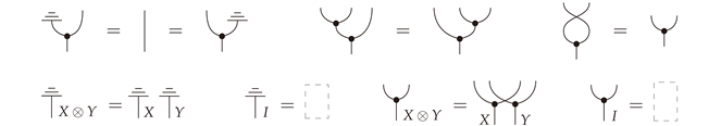 expressed using string diagrams. In addition, every morphism is natural with respect to
  in the sense that
  . Astateon X is a morphism , which is drawn as
  .
.
: X → I and ΔX ≡ : X → X X, all satisfying the following conditions
in the sense that . Astateon X is a morphism , which is drawn as .FinStoch is a Markov category (cf. Section 2). Although the definitions and results that follow are stated for stochastic maps, many hold for arbitrary Markov categories as well.
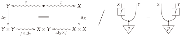
Definition A3
(Definition 7 in body). Let be a morphism in . The joint distribution associated with f is given by the following commutative diagram/string diagram equality:
Proposition A1
(Extending Proposition 4). The composable pair in is a.e. coalescable if and only if there exists a deterministic morphism such that
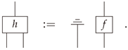
Proof.
Item (c) of Proposition 4 is a direct translation of this string diagram in terms of the composition of stochastic maps between finite sets. □
(A2) provides a categorical definition of mediator (cf. Definition 17).
Remark A2.
The morphism h in Proposition A1 is closely related to the abstract notion of conditionals in Markov categories ([3], Definition 11.5). Indeed, given morphisms and in a Markov category, ana.e. conditionalof F given Z is a morphism such that
 In our case, and h is the mediator. Therefore, a mediator is a deterministic (or at least a.e. deterministic) a.e. conditional for a specific morphism constructed from a pair of composable morphisms.
Remark A3.
In string-diagram notation, Lemma 3 reads
Example A1
(Example 2 in body). The mediator in this case may be given by
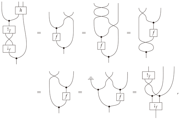
 The following string-diagrammatic calculation
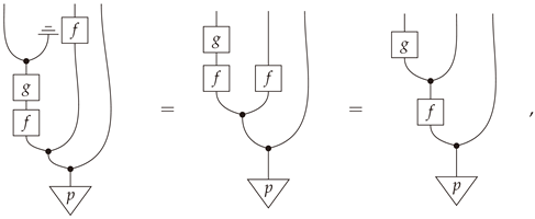 where p-a.e. determinism of f was used in the second equality, shows that (A2) holds.
Definition A4
(Definition 21 in body). Let be a morphism in . A Bayesian inverse of a morphism in is a morphism such that the following diagram commutes/string diagram equality holds:
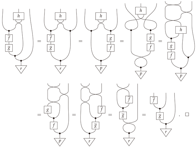
Alternative proof of Propotion 8.
A more abstract proof of Propotion 8 that is valid in an arbitrary classical Markov category can be given as follows:
Definition A5
(Definition 23 in body). Given a stochastic map , the bloom and shriek of f are given by
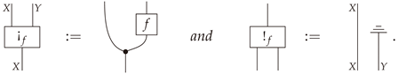
Diagrammatic proof of Propostion 10.
- (i)
- First,where the second equality holds by the very definition of the joint distribution .
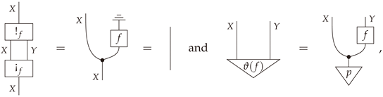
- (ii)
- Secondly,
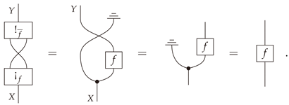
- (iii)
- Finally, set the mediator function to be the swap map. Thenwhich proves that the pair is coalescable. □
References
- Baez, J.C.; Fritz, T.; Leinster, T. A characterization of entropy in terms of information loss. Entropy 2011, 13, 1945–1957. [Google Scholar] [CrossRef]
- Cho, K.; Jacobs, B. Disintegration and Bayesian inversion via string diagrams. Math. Struct. Comp. Sci. 2019, 29, 938–971. [Google Scholar] [CrossRef] [Green Version]
- Fritz, T. A synthetic approach to Markov kernels, conditional independence and theorems on sufficient statistics. Adv. Math. 2020, 370, 107239. [Google Scholar] [CrossRef]
- Cover, T.M.; Thomas, J.A. Elements of Information Theory (Wiley Series in Telecommunications and Signal Processing); Wiley-Interscience: Hoboken, NJ, USA, 2006. [Google Scholar] [CrossRef]
- Gromov, M. Probability, Symmetry, Linearity. 2014. Available online: https://www.youtube.com/watch?v=aJAQVletzdY (accessed on 17 November 2020).
- Fritz, T. Probability and Statistics as a Theory of Information Flow. 2020. Available online: https://youtu.be/H4qbYPPcZU8 (accessed on 11 November 2020).
- Mac Lane, S. Categories for the Working Mathematician, 2nd ed.; Graduate Texts in Mathematics; Springer: New York, NY, USA, 1998; Volume 5. [Google Scholar] [CrossRef]
- Parzygnat, A.J. A functorial characterization of von Neumann entropy. arXiv 2020, arXiv:2009.07125. [Google Scholar]
- Fong, B. Causal Theories: A Categorical Perspective on Bayesian Networks. Master’s Thesis, University of Oxford, Oxford, UK, 2012. [Google Scholar]
- Parzygnat, A.J. Inverses, disintegrations, and Bayesian inversion in quantum Markov categories. arXiv 2020, arXiv:2001.08375. [Google Scholar]
- Smithe, T.S.C. Bayesian Updates Compose Optically. arXiv 2020, arXiv:2006.01631. [Google Scholar]
- Chang, H.H. An Introduction to Error-Correcting Codes: From Classical to Quantum. arXiv 2006, arXiv:0602157. [Google Scholar]
- Knill, E.; Laflamme, R.; Ashikhmin, A.; Barnum, H.; Viola, L.; Zurek, W.H. Introduction to Quantum Error Correction. arXiv 2002, arXiv:0207170. [Google Scholar]
- Selinger, P. A Survey of Graphical Languages for Monoidal Categories. Lect. Notes Phys. 2010, 289–355. [Google Scholar] [CrossRef] [Green Version]
Publisher’s Note: MDPI stays neutral with regard to jurisdictional claims in published maps and institutional affiliations. |
© 2021 by the authors. Licensee MDPI, Basel, Switzerland. This article is an open access article distributed under the terms and conditions of the Creative Commons Attribution (CC BY) license (https://creativecommons.org/licenses/by/4.0/).