Stochastic Analysis of Predator–Prey Models under Combined Gaussian and Poisson White Noise via Stochastic Averaging Method

Abstract

In the present paper, the statistical responses of two-special prey–predator type ecosystem models excited by combined Gaussian and Poisson white noise are investigated by generalizing the stochastic averaging method. First, we unify the deterministic models for the two cases where preys are abundant and the predator population is large, respectively. Then, under some natural assumptions of small perturbations and system parameters, the stochastic models are introduced. The stochastic averaging method is generalized to compute the statistical responses described by stationary probability density functions (PDFs) and moments for population densities in the ecosystems using a perturbation technique. Based on these statistical responses, the effects of ecosystem parameters and the noise parameters on the stationary PDFs and moments are discussed. Additionally, we also calculate the Gaussian approximate solution to illustrate the effectiveness of the perturbation results. The results show that the larger the mean arrival rate, the smaller the difference between the perturbation solution and Gaussian approximation solution. In addition, direct Monte Carlo simulation is performed to validate the above results.

1. Introduction

The Lotka–Volterra (LV) model [1] is a classic model for describing the interaction between the prey and predator in ecosystems with predator–prey relations [2,3]. Since the introduction of this model, several improved LV models have been investigated with consideration of different factors. Among those studies, the ones considering predator saturation and predator competition terms, respectively, have been introduced to characterize two special cases of the evolution of the ecosystems. The model with the predator saturation term describes a case where the preys are abundant, while the one with the predator competition term considers another case in which the predator population is very large compared with the prey population. The dynamics of these two models have been discussed in [1,4].

Moreover, the evolution of real-world biological systems usually suffers from unavoidable random perturbations in the natural environment [5,6,7,8,9]. Many investigations on the dynamics of predator–prey models with predator saturation and predator competition terms excited by stochastic perturbations have been reported [8,9,10,11,12,13,14]. In these studies, the stochastic perturbation is introduced as continuous stochastic excitations to disturb the birth rate of the prey and the death rate of the predator.

Nevertheless, in the environmental fluctuations, there are some drastic changes, including floods, earthquakes, tornados, or forest fires, which indicates that the evolutions of the ecosystem can be affected by unavoidable, sparse, discrete random jumps. Consequently, it is not appropriate to characterize the environmental effects by using only continuous random excitations. The combinations of continuous random processes and random jumps are viewed as more appropriate model for this case [15,16,17,18]. The ecosystem models excited by stochastic excitations with random jumps have been attracting increasing interests, and many reliable results have been obtained. In these studies, the Lévy process or jump-diffusion processes are commonly used in mathematical models to describe environmental perturbations with random jumps [19,20,21,22]. Most of them focus on the mathematical properties of the ecosystems, including the uniqueness, stability of the solutions, etc. [23,24,25,26,27]. However, for the prediction of the PDFs of the species populations, only the ecosystems enforced by stochastic processes with jumps have been investigated [28,29]. Therefore, more work needs to be done on deriving the stochastic responses of the ecosystems under stochastic excitations with random jumps.

The stochastic averaging method is an effective tool for investigating nonlinear systems excited by stochastic forcings. It was first applied to nonlinear systems under Gaussian white noise excitation [30,31,32], and then generalized to nonlinear systems with other types of stochastic excitations [33,34]. It has been successfully employed to study the stationary PDFs [6,7,8,9,11,12,28,35] and the optimal control [36] of species populations in ecosystems with small self-competition and small stochastic excitation. However, the solution of the ecosystem dynamics under continuous and random jump excitation by the stochastic average method has not yet been reported.

Inspired by this, here, we study predator–prey models with predator saturation and predator competition terms excited by combined Gaussian and Poisson noises. The governing equation for the solution of the stochastic model is approximately derived by applying the stochastic averaging method. Then, the statistical responses including the approximate PDFs and moments of the population densities are derived by solving the governing equation with a perturbation technique. Further, the effects of the system parameters as well as the stochastic excitations on the stationary responses are presented. The rest of the paper is organized as follows. Section 2 introduces two ecosystem models excited by combined Gaussian white noise and Poisson white noise and the averaged generalized Fokker–Planck–Kolmogorov (GFPK) equation. In Section 3, the effects of the parameters on the stochastic dynamics of the ecosystem are discussed. Finally, the conclusions are summarized in Section 4.

2. The Models

2.1. The Deterministic Models

In the present paper, we start from two deterministic prey–predator type ecosystems, one with an abundant prey population and the other with a large predator population, which can be viewed as generalizations of the LV model [1]. Although the two models are given based on different assumptions, fortunately we can define some new parameters to obtain a more general model that contains the two models as its special cases [8,37].

• Case 1: prey population is abundant

Consider the case where the prey is abundant. The model is given as

$$\begin{array}{l}{\dot{x}}_1=a{x}_1-s{x}_1^2-\frac{b{x}_1{x}_2}{1+A{x}_1},\\ {\dot{x}}_2=-c{x}_2+\frac{f{x}_1{x}_2}{1+A{x}_1}.\end{array}$$

(1)

where $x_1$ and $x_2$ are the prey and predator population densities, respectively; $a$ and $c$ represent the birth rate of the prey and the death rate of the predators. $-s{x}_1^2$ reveals the self-competition between the preys. The terms $\frac{b{x}_1{x}_2}{1+A{x}_1}$ and $\frac{f{x}_1{x}_2}{1+A{x}_1}$ in Equation (1) describe the interaction between the species [37]. These two interaction terms are proportional only to the predator population $x_2$, which implies that the consumption of the prey depends on the predator population and not on the prey population.

Model (1) can be reformulated in the following form

$$\begin{array}{l}{\dot{x}}_1=x_1\left[\overline{a}-\overline{b}{x}_2-\frac{s}{\overline{f}}\left(-c+\overline{f}{x}_1\right)+g_1\left(x_1,x_2\right)\right],\\ {\dot{x}}_2=x_2\left[-c+\overline{f}{x}_1+g_2\left(x_1,x_2\right)\right].\end{array}$$

(2)

with

$$g_1\left(x_1,x_2\right)=\frac{\overline{b}}{\overline{f}}A{x}_2\frac{\overline{f}{x}_1-c}{1+A{x}_1},g_2\left(x_1,x_2\right)=-A{x}_1\frac{\overline{f}{x}_1-c}{1+A{x}_1}$$

(3)

by introducing

$$\overline{f}=f-cA, \overline{a}=a-\frac{sc}{\overline{f}}=a-\frac{sc}{f-cA}, \overline{b}=\frac{\overline{f}b}{\overline{f}+cA}=\frac{b}{f}\left(f-cA\right).$$

(4)

At this time, Model (2) has two equilibrium points, one unstable point $\left(0,0\right)$ and one asymptotically stable point $\left(\overline{c}/\overline{f},\overline{a}/\overline{b}\right)$.

• Case 2: the predator population is large

When the population predator is large relative to the prey population, the prey–predator system can be modeled as

$$\begin{array}{l}{\dot{x}}_1=a{x}_1-s{x}_1^2-\frac{b{x}_1{x}_2}{1+B{x}_2},\\ {\dot{x}}_2=-c{x}_2+\frac{f{x}_1{x}_2}{1+B{x}_2}.\end{array}$$

(5)

In this case, the prey consumption depends only on the prey supplement. Compared with model (1) in Case 1, Model (5) has different interaction terms $\frac{b{x}_1{x}_2}{1+B{x}_2}$, $\frac{f{x}_1{x}_2}{1+B{x}_2}$, which imply that the prey growth rate and the predator death rate depend only on the prey supply. [8]. The other terms in (5) are the same as those in Equation (1).

By defining the new parameters

$$\overline{a}=a-\frac{sc}{\overline{f}}, \overline{f}=\frac{\overline{f}b}{\overline{b}+\overline{a}B}, \overline{b}=b-\overline{a}B,$$

(6)

Model (5) can be expressed in the form of Equation (2) with different nonlinear functions:

$$g_1\left(x_1,x_2\right)=-B{x}_2\frac{\overline{a}-\overline{b}{x}_2}{1+B{x}_2},g_2\left(x_1,x_2\right)=\frac{\overline{f}}{\overline{b}}B{x}_1\frac{\overline{a}-\overline{b}{x}_2}{1+B{x}_2}.$$

(7)

Some assumptions about the systems in Case 1 and Case 2 are needed for subsequent analysis. First, we consider the situation that the parameter $s$ in the self-competition term for both cases is small. It describes the situation that the prey population density is small, and the impact of the self-competitions term $-s{x}_1^2$ is small. Second, we assume the term $A{x}_1\ll 1$ for the Case 1. This assumption is consistent with the first one. Third, for Case 2, $B{x}_2\ll 1$ is also necessarily needed to meet the requirement of the first assumption. For the convenience of following analysis, a small and positive parameter $\epsilon$ is introduced and the parameters $s$, $A$ and $B$ in Equation (2) are replaced by ${\epsilon }^{2}s$, ${\epsilon }^{2}A$, and ${\epsilon }^{2}B$ to represent small values of these parameters. Thus, the mathematical model that we will investigate becomes

$$\begin{array}{l}{\dot{x}}_1=x_1\left[\overline{a}-\overline{b}{x}_2-\frac{{\epsilon }^{2}s}{\overline{f}}\left(-c+\overline{f}{x}_1\right)+{\epsilon }^2{g}_1\left(x_1,x_2\right)\right],\\ {\dot{x}}_2=x_2\left[\begin{array}{c}\\ \end{array}-c+\overline{f}{x}_1+{\epsilon }^2{g}_2\left(x_1,x_2\right)\right].\end{array}$$

(8)

with

$$g_1\left(x_1,x_2\right)=\frac{\overline{b}}{\overline{f}}A{x}_2\frac{\overline{f}{x}_1-c}{1+{\epsilon }^{2}A{x}_1},g_2\left(x_1,x_2\right)=-A{x}_1\frac{\overline{f}{x}_1-c}{1+{\epsilon }^{2}A{x}_1},$$

(9)

for Case 1 and with

$$g_1\left(x_1,x_2\right)=-B{x}_2\frac{\overline{a}-\overline{b}{x}_2}{1+{\epsilon }^{2}B{x}_2},g_2\left(x_1,x_2\right)=\frac{\overline{f}}{\overline{b}}B{x}_1\frac{\overline{a}-\overline{b}{x}_2}{1+{\epsilon }^{2}B{x}_2}.$$

(10)

for Case 2.

2.2. The Stochastic Model

We take the random environmental fluctuations into account in Equation (8). Gaussian white noise and Poisson white noise are adopted to model the random environmental fluctuations, which cause random changes in the growth rate of the prey and death rate of the predators. This means that the growth rate of the prey and the death rate of the predators in Equation (8) are changed as:

$$\overline{a}\to \overline{a}+\epsilon \left({\zeta }_1\left(t\right)+{\xi }_1\left(t\right)\right), c\to c+\epsilon \left({\zeta }_2\left(t\right)+{\xi }_2\left(t\right)\right),$$

(11)

Here, $\epsilon$ is the small parameter from Equation (8), which indicates that the random environmental influences are small. ${\zeta }_i\left(t\right)$$\left(i=1,2\right)$ are two independent Gaussian white noise excitations that are used to characterize the continuous environmental fluctuations. They have the following statistical characteristics:

$$E\left[{\zeta }_i\left(t\right)\right]=0, E\left[{\zeta }_i\left(t+\tau \right){\zeta }_i\left(t\right)\right]=2D_i\delta \left(\tau \right).$$

(12)

where $E[•]$ represents the mathematical expectation and $2D_i$ are the noise intensities. Moreover, two independent Poisson white noises ${\xi }_i\left(t\right)$$\left(i=1,2\right)$ are used to model the jump effects in the environment, which can be viewed as the formal derivatives of compound Poisson processes $C_i\left(t\right)$

$${\xi }_i\left(t\right)=\frac{d{C}_i\left(t\right)}{dt},C_i\left(t\right)={\displaystyle \sum _{k=1}^{N_i\left(t\right)}{Y}_{ik}U\left(t-t_{ik}\right)}, i=1,2.$$

(13)

In Equation (14), $N_i\left(t\right)$ denote Poisson counting processes with mean arrival rates ${\lambda }_i>0$. $Y_{ik}$ represent the random magnitudes of the impulses that obey Gaussian distributions with variances $E[Y_{ik}^2]$ and zero mean in the present paper. $U(•)$ is the unit step function. ${\lambda }_{i}E[Y_{ik}^2]$ are the intensities of the Poisson white noises. In addition, ${\zeta }_i\left(t\right)$ are also assumed to be independent with ${\xi }_i\left(t\right)$.

Consequently, the system that we will investigate can be described by the following Stratonovich stochastic differential equation (SDE) based on Equations (8) and (11),

$$\begin{array}{l}{\dot{X}}_1=X_1\left[\overline{a}-\overline{b}{X}_2-\frac{{\epsilon }^{2}s}{\overline{f}}\left(-c+\overline{f}{X}_1\right)+{\epsilon }^2{g}_1\left(X_1,X_2\right)+\epsilon {\zeta }_1\left(t\right)+\epsilon {\xi }_1\left(t\right)\right],\\ {\dot{X}}_2=X_2\left[-c+\overline{f}{X}_1+{\epsilon }^2{g}_2\left(X_1,X_2\right)+\epsilon {\zeta }_2\left(t\right)+\epsilon {\xi }_2\left(t\right)\right],\end{array}$$

(14)

where

$$g_1\left(X_1,X_2\right)=\frac{\overline{b}}{\overline{f}}A{X}_2\frac{\overline{f}{X}_1-c}{1+{\epsilon }^{2}A{X}_1},g_2\left(X_1,X_2\right)=-A{X}_1\frac{\overline{f}{X}_1-c}{1+{\epsilon }^{2}A{X}_1},$$

(15)

for Case 1 and

$$g_1\left(X_1,X_2\right)=-B{X}_2\frac{\overline{a}-\overline{b}{X}_2}{1+{\epsilon }^{2}B{X}_2},g_2\left(X_1,X_2\right)=\frac{\overline{f}}{\overline{b}}B{X}_1\frac{\overline{a}-\overline{b}{X}_2}{1+{\epsilon }^{2}B{X}_2},$$

(16)

for Case 2. Mathematically, the symbols $X_1\left(t\right)$ and $X_2\left(t\right)$ are used to represent the stochastic processes corresponding to the deterministic functions $x_1\left(t\right)$ and $x_2\left(t\right)$ in Equation (8).

Equation (14) can be transferred to the following Itô SDE by adding some correction terms as follows [38]

$$\begin{array}{ll}d{X}_1& =X_1\left[\overline{a}-\overline{b}{X}_2-\frac{s}{\overline{f}}\left(-c+\overline{f}{X}_1\right)+g_1\left(X_1,X_2\right)+\epsilon D_1\right]dt\\ & +\epsilon \sqrt{2D_1}{X}_{1}d{B}_1\left(t\right)+X_{1}d{C}_1\left(t\right)+X_1{\displaystyle \sum _{i=2}^{\infty }\frac{1}{i!}{\left(d{C}_1\left(t\right)\right)}^i},\\ d{X}_2& =X_2\left[-c+\overline{f}{X}_1+g_2\left(X_1,X_2\right)+\epsilon D_2\right]dt+\epsilon \sqrt{2D_2}{X}_{2}d{B}_2\left(t\right)\\ & +X_{2}d{C}_2\left(t\right)+X_2{\displaystyle \sum _{i=2}^{\infty }\frac{1}{i!}{\left(d{C}_2\left(t\right)\right)}^i},\end{array}$$

(17)

in which $X_1{\displaystyle \sum _{i=2}^{\infty }\frac{1}{i!}{\left(d{C}_1\left(t\right)\right)}^i}$ and $X_2{\displaystyle \sum _{i=2}^{\infty }\frac{1}{i!}{\left(d{C}_2\left(t\right)\right)}^i}$ are two correction terms. We introduce the integral form of the compound Poisson process by Poisson random measures for further analysis [39]

$$C_k\left(t\right)={\displaystyle {\int }_0^t{\displaystyle {\int }_{{\mathcal{Q}}_k}{Y}_k{\mathcal{P}}_k\left(dt,d{Y}_k\right)}}$$

(18)

where ${\mathcal{P}}_k\left(dt,d{Y}_k\right)$ are Poisson random measures and ${\mathcal{Q}}_k$ are the Poisson mark spaces. Based on the Poisson random measure, the differentiation of compound Poisson processes can be written as

$${\left(d{C}_k\left(t\right)\right)}^i={\displaystyle {\int }_0^t{\displaystyle {\int }_{{\mathcal{Q}}_k}{Y}_k^i{\mathcal{P}}_k\left(dt,d{Y}_k\right)}},i=1,2,\cdots$$

(19)

Then, the equivalent stochastic integro-differential equation (SIDE) of Equation (17) can be derived as [40]

$$\begin{array}{ll}d{X}_1& =X_1\left[\overline{a}-\overline{b}{X}_2-\frac{{\epsilon }^{2}s\left(-c+\overline{f}{X}_1\right)}{\overline{f}}+{\epsilon }^2{g}_1\left(X_1,X_2\right)+{\epsilon }^2{D}_1\right]dt\\ & +\epsilon \sqrt{2D_1}{X}_{1}d{B}_1\left(t\right)+{\displaystyle {\int }_{{\mathcal{Q}}_1}{\gamma }_{11}{\mathcal{P}}_1\left(dt,d{Y}_1\right)},\\ d{X}_2& =X_2\left[-c+\overline{f}{X}_1+{\epsilon }^2{g}_2\left(X_1,X_2\right)+{\epsilon }^2{D}_2\right]dt+\epsilon \sqrt{2D_2}{X}_{2}d{B}_2\left(t\right)\\ & +{\displaystyle {\int }_{{\mathcal{Q}}_2}{\gamma }_{22}{\mathcal{P}}_2\left(dt,d{Y}_2\right)},\end{array}$$

(20)

where

$${\gamma }_{11}=X_1{\displaystyle \sum _{i=1}^{\infty }\frac{{\epsilon }^i}{i!}{Y}_1^i} \mathrm{and} {\gamma }_{22}=X_2{\displaystyle \sum _{i=1}^{\infty }\frac{{\epsilon }^i}{i!}{Y}_2^i}.$$

(21)

In the remainder of this paper, the stochastic dynamics of the stochastic ecosystems will be analyzed based on Equation (20). Different from the deterministic system, the probability measures for the prey and predator population are needed to describe the random behavior of the system with random excitations. For the study of the stochastic problem, probability plays an important role. Thus, an important task here is to obtain the PDFs for both prey and predator population densities. In this paper, we focus on the long-term behavior of this stochastic model, namely, the stationary responses of Equation (14). To derive the stationary PDFs, we use a stochastic averaging method as described below.

2.3. The Stochastic Averaging

Without considering the random excitations and the nonlinear function $g_i\left(x_1,x_2\right)$ (I = 1, 2) and letting the self-competition term be 0, Equation (20) reduces to the famous LV model

$$\begin{array}{l}{\dot{x}}_1=x_1\left(\overline{a}-\overline{b}{x}_2\right),\\ {\dot{x}}_2=x_2\left(-c+\overline{f}{x}_1\right).\end{array}$$

(22)

It is known [1] that the system (22) has periodic trajectories that can be defined by

$$r\left(x_1,x_2\right)=\overline{f}{x}_1-c-c\ln \frac{\overline{f}{x}_1}{c}+\overline{b}{x}_2-\overline{a}-\overline{a}\ln \frac{\overline{b}{x}_2}{\overline{a}}=Q,$$

(23)

where $Q$ is a constant and $r\left(x_1,x_2\right)=0$ at both the unstable equilibrium point $\left(0,0\right)$ and the stable non-asymptotic equilibrium point $\left(\overline{c}/\overline{f},\overline{a}/\overline{b}\right)$ of Equation (22). This means that Equation (23) is the first integral of the system (22) for any positive value $Q$ [1]. The period of the periodic trajectories with constant $Q$ is determined by

$$T\left(Q\right)={\displaystyle \oint dt}={\displaystyle \oint \frac{d{x}_2}{x_2\left(\overline{f}{x}_1-c\right)}=}{\displaystyle \oint \frac{d{x}_1}{x_1\left(\overline{a}-\overline{b}{x}_2\right)}}.$$

(24)

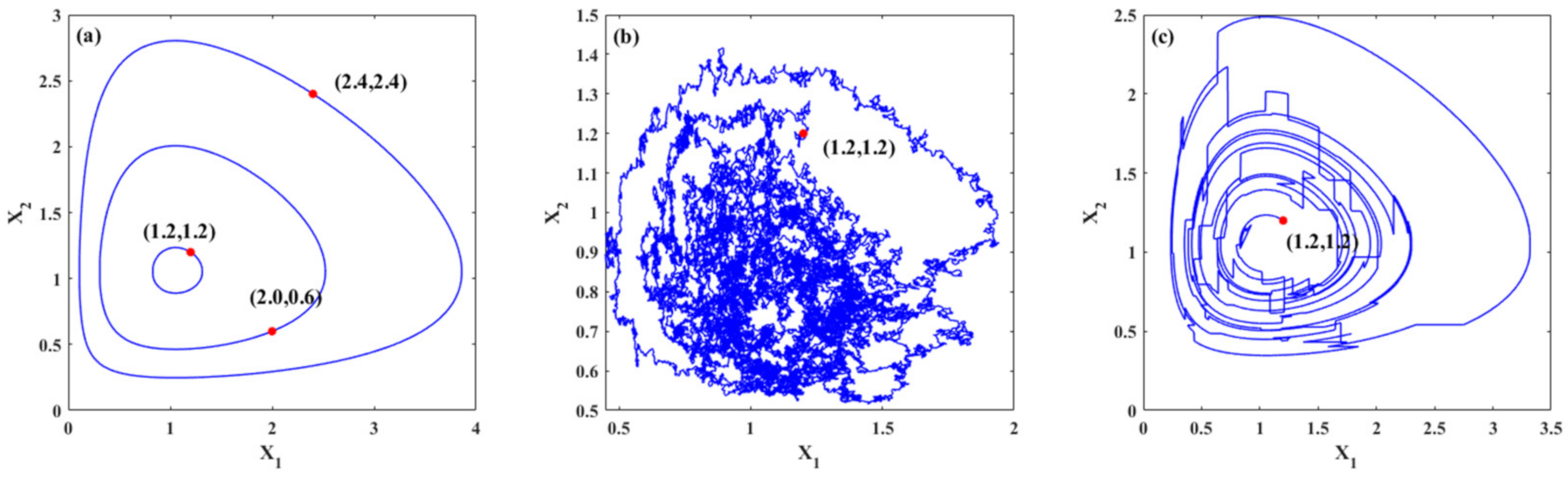
Figure 1 demonstrates the trajectories of the system for three cases. Figure 1a shows the periodic trajectories for system (22) with different initial values. For different initial values, different closed orbits are obtained, namely, periodic solutions. Figure 1b,c show the random trajectories for system (22) under Gaussian white noise and Poisson white noise, respectively. It is known that stochastic excitation has a significant influence on the dynamics of the ecosystems. The trajectories of the system under stochastic excitations are random. Moreover, the trajectory changes with continuous slight jumps for the system with Gaussian white noises, while for the system excited by Poisson white noises, the trajectory includes some large jumps, which demonstrates the influences of different stochastic excitations on the trajectories. It can also be seen in these figures that large population densities of species may evolve into smaller population densities with the evolution of time. For an ecosystem, a smaller population density means that the population is more likely to die out, which means that the system is relatively fragile or unstable.

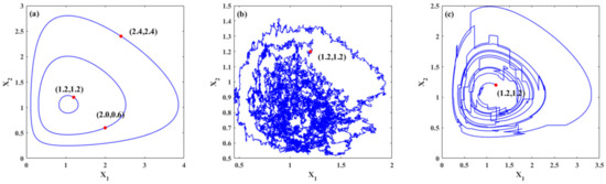
Figure 1. Typical trajectories of the systems. (a) Deterministic trajectories of system (22) with different initial values; (b) one trajectory of the system under Gaussian white noises only with initial value (1.2,1.2); (c) one trajectory of the system under Poisson white noises only with initial value (1.2,1.2).

Replacing the variables $x_1$ and $x_2$ by stochastic processes $X_1$ and $X_2$ in Equation (23), the random counterpart of the first integral (23) can be obtained as

$$R\left(t\right)=R\left(X_1,X_2\right)=\overline{f}{X}_1-c-c\ln \frac{\overline{f}{X}_1}{c}+\overline{b}{X}_2-\overline{a}-\overline{a}\ln \frac{\overline{b}{X}_2}{\overline{a}}.$$

(25)

Based on the stochastic chain rule [39], the differential form of the first integral is given as

$$\begin{array}{ll}dR\left(t\right)& =\left(\overline{f}{X}_1-c\right)\left[-\frac{{\epsilon }^{2}s}{\overline{f}}\left(-c+\overline{f}{X}_1\right)+{\epsilon }^2{g}_1\left(X_1,X_2\right)+{\epsilon }^2{D}_1+{\epsilon }^{2}c{D}_1\right]dt\\ & +\left(\overline{b}{X}_2-\overline{a}\right)\left[{\epsilon }^2{g}_2\left(X_1,X_2\right)+{\epsilon }^2{D}_2+{\epsilon }^{2}a{D}_2\right]dt+\epsilon \sqrt{2D_1}\left(\overline{f}{X}_1-c\right)d{B}_1\left(t\right)\\ & +\epsilon \sqrt{2D_2}\left(\overline{b}{X}_2-\overline{a}\right)d{B}_2\left(t\right)+{\displaystyle {\int }_{{\mathcal{Q}}_1}\left[\overline{f}{\gamma }_{11}-c\ln \left(1+\frac{{\gamma }_{11}}{X_1}\right)\right]}{\mathcal{P}}_1\left(dt,d{Y}_1\right)\\ & +{\displaystyle {\int }_{{\mathcal{Q}}_2}\left[\overline{b}{\gamma }_{22}-\overline{a}\ln \left(1+\frac{{\gamma }_{22}}{X_2}\right)\right]}{\mathcal{P}}_2\left(dt,d{Y}_2\right).\end{array}$$

(26)

Taking the Taylor expansions of $\ln \left(1+{\gamma }_{11}/X_1\right)$ and $\ln \left(1+{\gamma }_{22}/X_2\right)$, and substituting them in Equation (26), one arrives at

$$\begin{array}{ll}dR\left(t\right)& =\left(\overline{f}{X}_1-c\right)\left[-\frac{{\epsilon }^{2}s}{\overline{f}}\left(-c+\overline{f}{X}_1\right)+{\epsilon }^2{g}_1\left(X_1,X_2\right)+{\epsilon }^2{D}_1+{\epsilon }^{2}c{D}_1\right]dt\\ & +\left(\overline{b}{X}_2-\overline{a}\right)\left[{\epsilon }^2{g}_2\left(X_1,X_2\right)+{\epsilon }^2{D}_2+{\epsilon }^{2}a{D}_2\right]dt\\ & +\epsilon \sqrt{2D_1}\left(\overline{f}{X}_1-c\right)d{B}_1\left(t\right)+\epsilon \sqrt{2D_2}\left(\overline{b}{X}_2-\overline{a}\right)d{B}_2\left(t\right)\\ & +{\displaystyle {\int }_{{\mathcal{Q}}_1}\left[\epsilon A_{11}{Y}_1+{\epsilon }^2{A}_{12}{Y}_1^2+{\epsilon }^3{A}_{13}{Y}_1^3+{\epsilon }^4{A}_{14}{Y}_1^4\text{+}\cdots \right]}{\mathcal{P}}_1\left(dt,d{Y}_1\right)\\ & +{\displaystyle {\int }_{{\mathcal{Q}}_2}\left[\epsilon A_{21}{Y}_2+{\epsilon }^2{A}_{22}{Y}_2^2+{\epsilon }^3{A}_{23}{Y}_2^3+{\epsilon }^4{A}_{24}{Y}_2^4\text{+}\cdots \right]}{\mathcal{P}}_2\left(dt,d{Y}_2\right).\end{array}$$

(27)

in which

$$\begin{gathered} A_{11}=\overline{f}{X}_1-c; A_{12}=\frac{\overline{f}{X}_1}{2}; A_{13}=\frac{\overline{f}{X}_1}{6}; A_{14}=\frac{\overline{f}{X}_1}{24}; \\ {A}_{21}=\overline{b}{X}_2-\overline{a}; A_{22}=\frac{\overline{b}{X}_2}{2}; A_{23}=\frac{\overline{b}{X}_2}{6}; A_{24}=\frac{\overline{b}{X}_2}{24}. \end{gathered}$$

Replacing $X_1$ in Equation (20) by $R\left(t\right)$ yields a new system governed by Equation (27) and the second equation of Equation (20). $R\left(t\right)$ is a slowly varying variable since $\epsilon$ is a small parameter, while $X_i$ are rapidly varying variables. Based on the stochastic averaging method proposed by [41,42], one can derive the averaged GFPK equation for $R\left(t\right)$ as

$$\begin{array}{ll}\frac{\partial }{\partial t}p\left(r,t\right)& =-\frac{\partial }{\partial r}\left({\overline{A}}_{1}p\left(r,t\right)\right)+\frac{1}{2!}\frac{{\partial }^2}{\partial r^2}\left({\overline{A}}_{2}p\left(r,t\right)\right)-\frac{1}{3!}\frac{{\partial }^3}{\partial r^3}\left({\overline{A}}_{3}p\left(r,t\right)\right)\\ & +\frac{1}{4!}\frac{{\partial }^4}{\partial r^4}\left({\overline{A}}_{4}p\left(r,t\right)\right)+O\left({\epsilon }^5\right),\end{array}$$

(28)

where $p\left(r,t\right)$ is the PDF of $R\left(t\right)$ at time $t$. $O({\epsilon }^5)$ represents the terms of ${\epsilon }^5$ and higher, which contains an infinite number of terms of GFPK equation with small magnitude due to the increasing powers of $\epsilon$. The other parameters of Equation (28) are given as

$${\overline{A}}_1={\epsilon }^2{\overline{A}}_{11}+{\epsilon }^4{\overline{A}}_{12},$$

(29)

$${\overline{A}}_{11}={⟨U_0+A_{12}{\lambda }_1\left[Y_1^2\right]+A_{22}{\lambda }_2\left[Y_2^2\right]⟩}_t,$$

(30)

$${\overline{A}}_{12}={⟨A_{14}{\lambda }_1\left[Y_1^4\right]+A_{24}{\lambda }_2\left[Y_2^4\right]⟩}_t,$$

(31)

$$\begin{array}{c}{U}_0=\left(f{X}_1-c\right)\left[-\frac{s}{f}\left(-c+f{X}_1\right)+g_1\left(X_1,X_2\right)+D_1\left(1+c\right)\right]\\ +\left(b{X}_2-a\right)\left[g_2\left(X_1,X_2\right)+D_2\left(1+a\right)\right],\end{array}$$

(32)

$${\overline{A}}_2={\epsilon }^2{\overline{A}}_{21}+{\epsilon }^4{\overline{A}}_{22},$$

(33)

$${\overline{A}}_{21}={⟨A_{11}^2\left(2D_1+{\lambda }_{1}E\left[Y_1^2\right]\right)+A_{21}^2\left(2D_2+{\lambda }_{2}E\left[Y_2^2\right]\right)⟩}_t,$$

(34)

$${\overline{A}}_{22}={⟨\left(A_{12}^2+2A_{11}{A}_{13}\right){\lambda }_{1}E\left[Y_1^4\right]+\left(A_{22}^2+2A_{21}{A}_{23}\right){\lambda }_{2}E\left[Y_2^4\right]⟩}_t,$$

(35)

$${\overline{A}}_3={\epsilon }^4{\overline{A}}_{31}={\epsilon }^4{⟨3A_{11}^2{A}_{12}{\lambda }_{1}E\left[Y_1^4\right]+3A_{21}^2{A}_{22}{\lambda }_{2}E\left[Y_2^4\right]⟩}_t,$$

(36)

$${\overline{A}}_4={\epsilon }^4{\overline{A}}_{41}={\epsilon }^4{⟨A_{11}^4{\lambda }_{1}E\left[Y_1^4\right]+A_{21}^4{\lambda }_{2}E\left[Y_2^4\right]⟩}_t,$$

(37)

where the symbol ${⟨\left[ \right]⟩}_t$ means the time average in one quasi-period, which is defined as

$${⟨\left[ \right]⟩}_t=\frac{1}{T}{\displaystyle \oint \left[ \right]dt}=\frac{1}{T}{\displaystyle \oint \frac{\left[ \right]d{x}_2}{x_2\left(f{x}_1-c\right)}=}\frac{1}{T}{\displaystyle \oint \frac{\left[ \right]d{x}_1}{x_1\left(a-b{x}_2\right)}},$$

(38)

where $T$ is the period given in Equation (24).

It can be found from Equations (29)–(37) that the coefficients consist of terms of order ${\epsilon }^2$ and ${\epsilon }^4$. In the absence of terms of order ${\epsilon }^4$ and higher in Equation (28) the averaged GFPK Equation (28) will reduce to the averaged FPK equation for the system under only Gaussian white noises ${\zeta }_i\left(t\right)$ with intensities $(2D_i+{\lambda }_{i}E[Y_i^2])$$(i=1,2)$. By solving this reduced FPK equation, one can obtain the Gaussian approximation solution for the averaged GFPK equations. However, the Gaussian approximation solution is not a proper approximation for small values of $\lambda$ for Poisson white noise with the same noise intensity since the influence of term of order ${\epsilon }^4$ in Equation (28) cannot be ignored. Therefore, more terms of the GFPK equations should be considered to obtain a more accurate solution when dealing with the system with Poisson white noise.

3. The Approximate Stationary Responses

The PDFs of the population densities are obtained by solving the averaged GFPK Equation (28) with certain boundary and initial conditions. In the present paper, only the long-term behaviors of the ecosystem are studied. A perturbation technique [43] is applied to derive the stationary PDFs $p_R\left(r\right)$ for $R\left(t\right)$ by solving the following reduced averaged GFPK equation

$$\begin{array}{ll}0& =-\frac{\partial }{\partial r}\left({\overline{A}}_1{p}_R\left(r\right)\right)+\frac{1}{2!}\frac{{\partial }^2}{\partial r^2}\left({\overline{A}}_2{p}_R\left(r\right)\right)-\frac{1}{3!}\frac{{\partial }^3}{\partial r^3}\left({\overline{A}}_3{p}_R\left(r\right)\right)\\ & +\frac{1}{4!}\frac{{\partial }^4}{\partial r^4}\left({\overline{A}}_4{p}_R\left(r\right)\right)+O\left({\epsilon }^5\right),\end{array}$$

(39)

A second-order perturbation solution

$$p_R\left(r\right)=p_0\left(r\right)+\epsilon p_1\left(r\right)+{\epsilon }^2{p}_2\left(r\right)$$

(40)

is adopted here to derive the approximate solution of Equation (39). By substituting Equation (40) into Equation (39) and putting terms of the same order of $\epsilon$ together, the equations for $p_0\left(r\right)$, $p_1\left(r\right)$, $p_2\left(r\right)$ are given as

$$-\frac{\partial }{\partial r}\left({\epsilon }^2{\overline{A}}_{11}{p}_0\left(r\right)\right)+\frac{1}{2}\frac{{\partial }^2}{\partial r^2}\left({\epsilon }^2{\overline{A}}_{12}{p}_0\left(r\right)\right)=0$$

(41)

$$-\frac{\partial }{\partial r}\left({\epsilon }^3{\overline{A}}_{11}{p}_1\left(r\right)\right)+\frac{1}{2}\frac{{\partial }^2}{\partial r^2}\left({\epsilon }^3{\overline{A}}_{12}{p}_1\left(r\right)\right)=0$$

(42)

$$\begin{array}{l}-\frac{\partial }{\partial r}\left({\epsilon }^4{\overline{A}}_{11}{p}_2\left(r\right)\right)+\frac{1}{2}\frac{{\partial }^2}{\partial r^2}\left({\epsilon }^4{\overline{A}}_{12}{p}_2\left(r\right)\right)\\ =\frac{\partial }{\partial r}\left({\epsilon }^4{\overline{A}}_{12}{p}_0\left(r\right)\right)-\frac{1}{2}\frac{{\partial }^2}{\partial r^2}\left({\epsilon }^4{\overline{A}}_{22}{p}_0\left(r\right)\right)\\ +\frac{1}{3!}\frac{{\partial }^3}{\partial r^3}\left({\epsilon }^4{\overline{A}}_{31}{p}_0\left(r\right)\right)-\frac{1}{4!}\frac{{\partial }^4}{\partial r^4}\left({\epsilon }^4{\overline{A}}_{41}{p}_0\left(r\right)\right)\end{array}$$

(43)

It can be seen from Equation (41) that $p_0\left(r\right)$ is the solution for the system excited by Gaussian white noise with the same noise intensity, namely, approximate Gaussian solutions for the system excited by Poisson white noise. By solving Equations (41)–(43) step-by-step, the second-order perturbation solution (40) can be obtained. Then, the approximate stationary joint PDFs $p_{X_1{X}_2}\left(x_1,x_2\right)$ take the form

$$p_{X_1{X}_2}\left(x_1,x_2\right)=\frac{p_R\left(r\right)}{x_1{x}_{2}T\left(r\right)}.$$

(44)

The marginal PDFs and moments of $X_1$ and $X_2$ can be calculated from Equation (44), such as

$$p_{X_1}\left(x_1\right)={\displaystyle {\int }_0^{\infty }{p}_{X_1{X}_2}\left(x_1,x_2\right)}d{x}_2,p_{X_2}\left(x_2\right)={\displaystyle {\int }_0^{\infty }{p}_{X_1{X}_2}\left(x_1,x_2\right)}d{x}_1$$

(45)

$$E\left[X_1\right]={\displaystyle {\int }_0^{\infty }{x}_1{p}_{X_1}\left(x_1\right)}d{x}_1, Var\left(X_1\right)={\displaystyle {\int }_0^{\infty }{\left[x_1-E(X_1)\right]}^2}d{x}_1$$

(46)

$$E\left[X_2\right]={\displaystyle {\int }_0^{\infty }{x}_2{p}_{X_2}\left(x_2\right)}d{x}_2,Var\left(X_2\right)={\displaystyle {\int }_0^{\infty }{\left[x_2-E(X_2)\right]}^2}d{x}_2$$

(47)

Furthermore, when the Poisson white noise intensity is 0, the method developed in this paper reduces to the case excited by Gaussian white noise. The effects of the Gaussian noise on the dynamics of the ecosystems have been studied by Cai [7]. Therefore, in the following subsections, we focus on the influence of the system parameters and Poisson white noise parameters on the stationary statistics.

3.1. The Influence of System Parameters

In this section, the influences of system parameters on the model (14) for Case 1 and Case 2 are shown in Figure 2, Figure 3, Figure 4, Figure 5, Figure 6, Figure 7, Figure 8 and Figure 9. The stochastic properties of population densities of the prey and predator can be calculated from Equations (44)–(47).

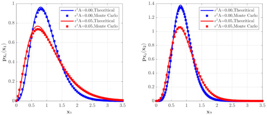
Figure 2. The PDFs of $X_1$ for the model with predator saturation term (Case 1) for different ${\epsilon }^{2}A$ values.

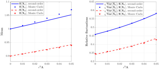
Figure 3. The means and relative fluctuations of $X_1$ and $X_2$ and $X_2$ for the model with predator saturation term (Case 1) for different ${\epsilon }^{2}A$ value. The parameters are the same as those in Figure 2 except for ${\lambda }_i=1.0$, $E[Y_i^2]=0.01$, $i=1,2$.

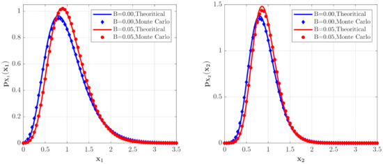
Figure 4. The PDFs of $X_1$ and $X_2$ for the model with the predator competition term (Case 2) for different ${\epsilon }^{2}B$ values. The parameters are the same as those in Figure 2 except for ${\lambda }_i=0.5$, ${\epsilon }^{2}E[Y_i^2]=0.02$, $i=1,2$.

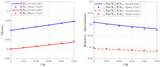
Figure 5. The means and relative fluctuations of $X_1$ and $X_2$ for the model with the predator competition term (Case 2) for different ${\epsilon }^{2}B$ values. The parameters are the same as those in Figure 4 except ${\lambda }_i=1.0$, ${\epsilon }^{2}E[Y_i^2]=0.01$, $i=1,2$.

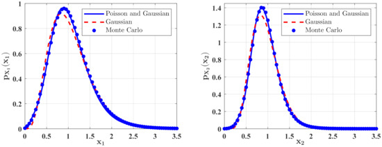
Figure 6. The PDFs of $X_1$ and $X_2$ for Case 1. The parameters are the same as those in Figure 2 except for ${\epsilon }^{2}A=0.05$, $2{\epsilon }^2{D}_i=0.001$, $\lambda ={\lambda }_i=0.1$, ${\epsilon }^{2}E[Y^2]={\epsilon }^{2}E[Y_i^2]=0.08$, $i=1,2$.

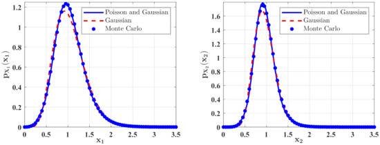
Figure 7. The PDFs of $X_1$ and $X_2$ for Case 2. The parameters are the same as those in Figure 4 except for ${\epsilon }^{2}s=0.08$, ${\epsilon }^{2}B=0.05$, $2{\epsilon }^2{D}_i=0.001$, $\lambda ={\lambda }_i=0.2$, ${\epsilon }^{2}E[Y^2]={\epsilon }^{2}E[Y_i^2]=0.04$, $i=1,2$.

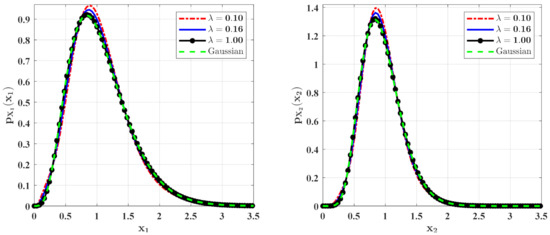
Figure 8. The PDFs of $X_1$ and $X_2$ for Case 1 with different mean arrival rate $\lambda$. The other parameters are the same as those in Figure 6.

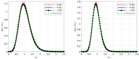
Figure 9. The PDFs of $X_1$ and $X_2$ for Case 2 with different mean arrival rate $\lambda$. The other parameters are the same as those in Figure 7.

Case 1: prey is abundant compared with the predator

The effects of the parameter ${\epsilon }^{2}A$ in the predator saturation term of Equation (15) on the stationary PDFs of the species are shown in Figure 2. The PDF $p_{X_1}\left(x_1\right)$ of the population density of the prey $X_1\left(t\right)$ and the PDF of the population density of the predators $X_2$ are calculated with the following parameters $a=1.0$, $b=1.0$, $c=0.5$, $f=0.5$, ${\epsilon }^{2}s=0.1$, $2{\epsilon }^2{D}_i=0.005$, ${\lambda }_i=0.5$, ${\epsilon }^{2}E[Y_i^2]=0.02$, $i=1,2$, and two different values of ${\epsilon }^{2}A$. One can see from Figure 2 that the occurrence of the predator saturation influences the system behavior significantly. Compared with the case of ${\epsilon }^{2}A=0.0$, the maxima of the PDFs of the species population densities become lower, and the probabilities for both small and large populations increase for ${\epsilon }^{2}A=0.05$. This means that the ecosystem becomes more unstable for ${\epsilon }^{2}A=0.05$. This is reasonable in the real world. Since the parameter ${\epsilon }^{2}A$ represents the case of large prey population, it is obvious that the ecosystem is more unstable when this extreme case occurs. The solid lines in Figure 2 show the second-order perturbation solutions, while the discrete points denote the results obtained from Monte Carlo simulation. The good agreement between these two results shows the effectiveness of the second-order perturbation solution.

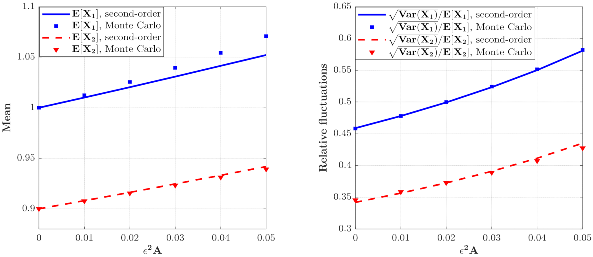
The effect of ${\epsilon }^{2}A$ on the moments of the population densities of prey and predators which can be calculated from Equations (46) and (47) are depicted in Figure 3. It can be seen that the curves for the means and relative fluctuations $\sqrt{Var\left(X_i\right)}/E\left[X_i\right]$ of the population densities of both species increase monotonously. This means that the ecosystem fluctuates more strongly for larger value of ${\epsilon }^{2}A$, which implies a more unstable system.

Case 2: predator population is large

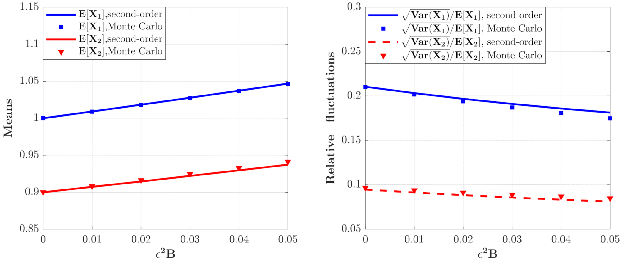
Figure 4 depicts the PDFs of $X_1$ and $X_2$ for the model in Case 2 for different ${\epsilon }^{2}B$ values. It is found that the maxima of the PDFs for the case of ${\epsilon }^{2}B=0.05$ are larger and the probability in this case is more concentrated. Figure 5 shows the mean and relative fluctuation of the species population of the ecosystem. It can be seen that the mean value of the prey and predator increase with increase of the ${\epsilon }^{2}B$ value, while the relative fluctuation curves decrease with increasing the value of ${\epsilon }^{2}B$, implying a more stable ecosystem. The results of the Monte Carlo simulations are also given in Figure 4 and Figure 5 to validate the results of the proposed method.

3.2. The Influence of Poisson White Noise

In this section, we focus on the influences of the parameters of the Poisson white noises, namely mean arrival rate $\lambda$ and the variance of amplitude $E[Y^2]$.

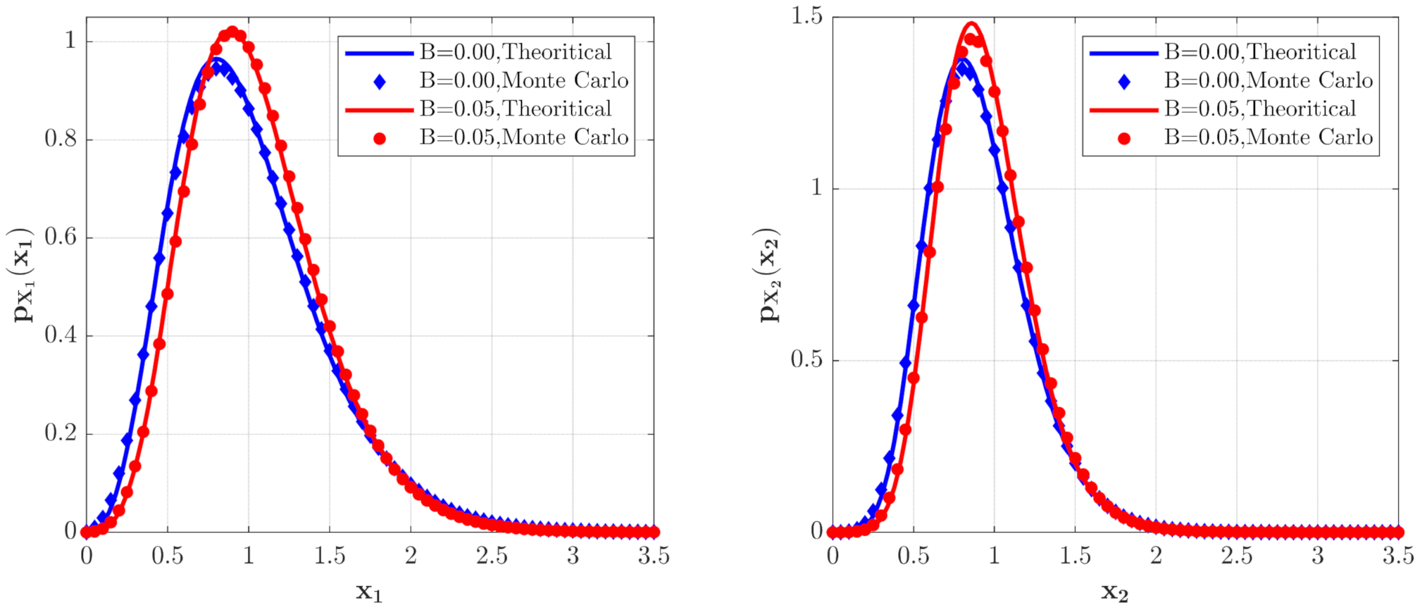
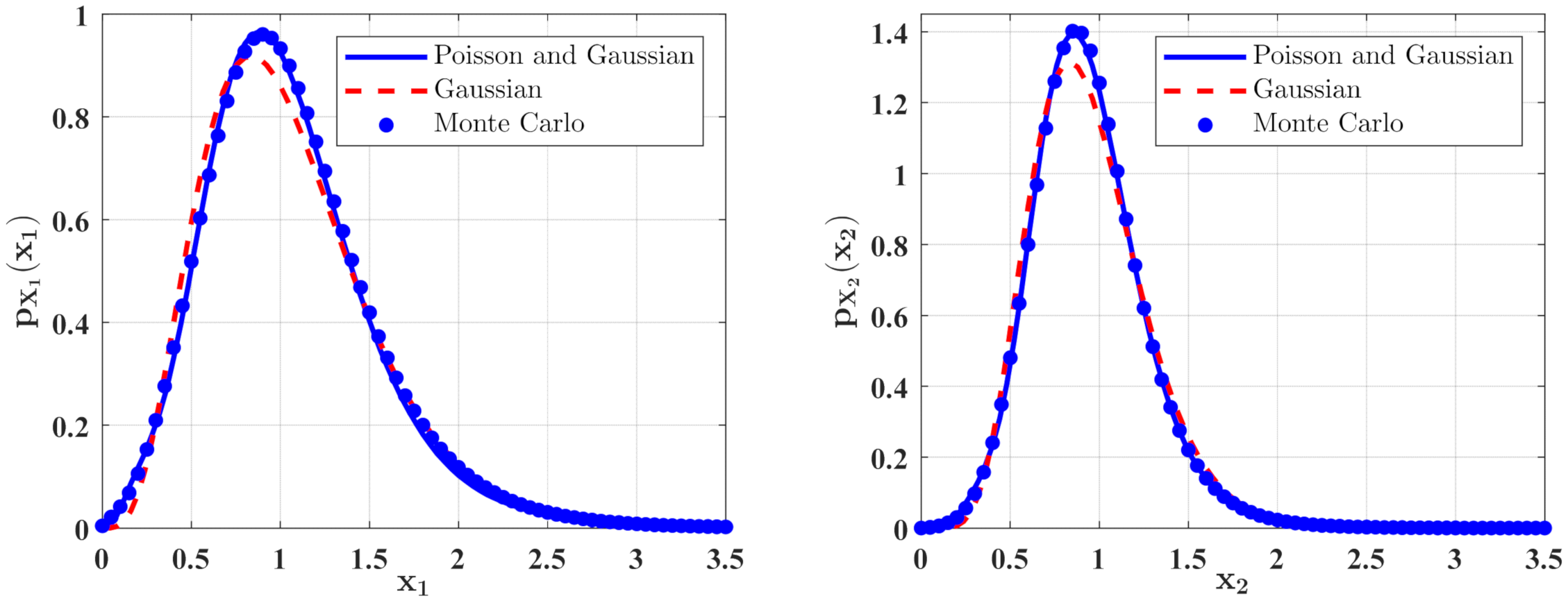
In Figure 6 and Figure 7, some numerical calculations have been performed to obtain the PDFs of predator and prey population densities in the model (14) for Case 1 and Case 2, respectively. In these figures, the second-order perturbation results are represented by the solid lines. The dashed lines are the approximate Gaussian solutions. The Monte Carlo results are plotted as dotted lines. It is found that the PDFs obtained by the present method are closer to the Monte Carlo simulation than the approximate Gaussian solutions. The maxima of the stationary PDFs for the system with both Gaussian and Poisson white noise are higher than for the approximate Gaussian solutions. This means that the second-order perturbation solutions have higher accuracy than the Gaussian approximation solution.

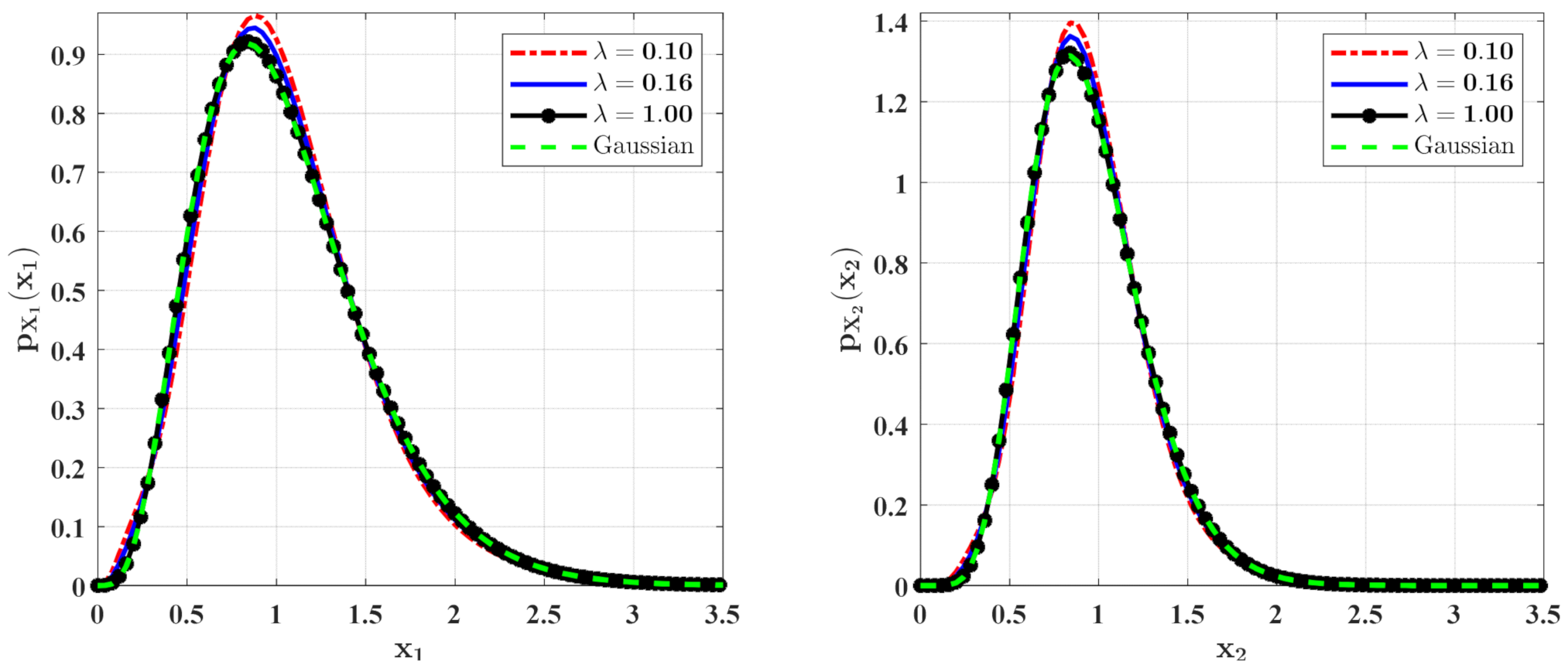
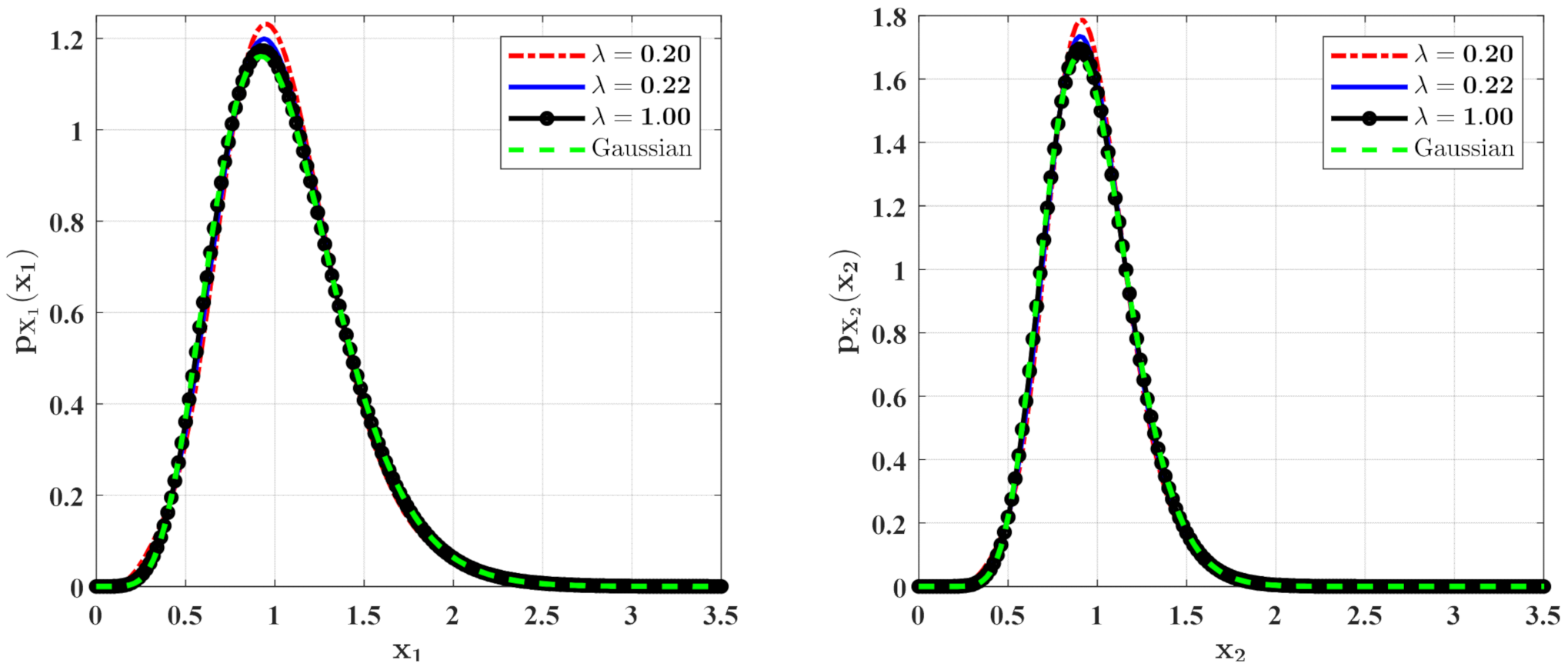
Figure 8 and Figure 9 show the influences of $\lambda$ of the Poisson white noises on the stationary PDFs when the Poisson white noise intensity $\lambda E[Y^2]$ is kept constant. It is observed from these figures that with the increase of $\lambda$, the maxima of the PDFs decrease and the PDFs for population densities of prey and predator approach the ones for the system with the same intensity of Gaussian white noise excitation. To see this clearly, we define the $L_2$ error norm between the PDFs for the system with Poisson white noise and the Gaussian approximation solution as

$$l2\left(x_i\right)={\displaystyle {\int }_0^{+\infty }{\left(p_{X_i}\left(x_i\right)-p_{x_i}^G\left(x_i\right)\right)}^{2}d{x}_i}$$

(48)

where $p_{X_i}\left(x_i\right)$ are the second-order perturbation PDFs for $X_i$ and $p_{x_i}^G\left(x_i\right)$ are the Gaussian approximation solutions. We calculate the errors for different $\lambda$ for Case 1 (Table 1) and Case 2 (Table 2). It can also be seen from these tables that with the increase of $\lambda$, the error decreases significantly, which also verifies our above conclusion.

Table 1. Error $l2\left(x_i\right)$ for PDFs in Case 1.

$\mathit{\lambda }$	0.05	0.08	0.2	0.4	0.6	0.8	1.0	2.0
l2(x1)	1.19 × 10−2	7.61 × 10−3	9.90 × 10−4	4.52 × 10−4	1.03 × 10−4	3.22 × 10−5	1.84 × 10−5	9.37 × 10−8
l2(x2)	1.54 × 10−2	9.78 × 10−3	1.27 × 10−3	5.85 × 10−4	1.33 × 10−4	4.10 × 10−5	2.34 × 10−5	1.28 × 10−7

Table 2. Error $l2\left(x_i\right)$ for PDFs in Case 2.

$\mathit{\lambda }$	0.05	0.08	0.2	0.4	0.6	0.8	1.0	2.0
l2(x1)	4.39 × 10−2	1.78 × 10−2	4.20 × 10−3	1.21 × 10−3	6.72 × 10−4	1.10 × 10−4	3.81 × 10−5	3.05 × 10−7
l2(x2)	6.05 × 10−2	2.44 × 10−2	5.72 × 10−3	1.65 × 10−3	9.29 × 10−4	1.50 × 10−4	5.19 × 10−5	4.21 × 10−7

4. Conclusions

In the present paper, we have investigated the statistical responses of a stochastic prey–predator type model for the possible situations of sufficient prey supply and a large predator population. The statistical responses of the species population, including the approximate stationarity PDFs and moments, have been obtained by a stochastic averaging and a perturbation technique. It can be found that, for the system with abundant prey, the increase of the parameter ${\epsilon }^{2}A$ describing the saturation of the predator population from 0 to 0.5 leads to the increase of population fluctuations, which implies that the system becomes unstable. However, for the system where the predator population is large, the increase of the parameter ${\epsilon }^{2}B$ describing the competition of predators for prey has the opposite effect. In addition, we have paid special attention to the effect of the mean arrival rate $\lambda$ of the Poisson white noise. The influence of Poisson white noise on the system tends to approach the influence of Gaussian white noise with the same noise intensity when the $\lambda$ increases from 0.05 to 2.0.

Although only two types of ecosystems with combined Gaussian and Poisson white noise have been investigated in this paper, our approaches can be applied to other ecosystem models. Except for the stochastic response of the ecosystem being investigated, the stochastic optimal control or extinction problem are also worth studying.

References

- Bazykin, A.D. Nonlinear Dynamics of Interacting Populations; World Scientific: Singapore, 1998. [Google Scholar]
- Ma, Z.; Wang, W. Asymptotic behavior of predator–prey system with time dependent coefficients. Appl. Anal. 1989, 34, 79–90. [Google Scholar]
- Chen, F.; Shi, C. Global attractivity in an almost periodic multi-species nonlinear ecological model. Appl. Math. Comput. 2006, 180, 376–392. [Google Scholar] [CrossRef]
- Rosenzweig, M.L.; Macarthur, R.H. Graphical representation and stability conditions of predator-prey Interactions. Am. Nat. 1963, 97, 209–223. [Google Scholar] [CrossRef]
- Xu, Y.; Xu, W.; Mahmoud, G.M. On a complex beam-beam interaction model with random forcing. Physica A 2004, 336, 347–360. [Google Scholar] [CrossRef]
- Khasminskii, R.Z.; Klebaner, F.C. Long term behavior of solutions of the Lotka-Volterra system under small random perturbations. Ann. Appl. Probab. 2001, 11, 952–963. [Google Scholar] [CrossRef]
- Cai, G.Q.; Lin, Y.K. Stochastic analysis of the Lotka-Volterra model for ecosystems. Phys. Rev. E Stat. Nonlinear Soft Matter Phys. 2004, 70 Pt 1, 041910. [Google Scholar] [CrossRef]
- Cai, G.Q.; Lin, Y.K. Stochastic analysis of predator-prey type ecosystems. Ecol. Complex. 2007, 4, 242–249. [Google Scholar] [CrossRef]
- Cai, G.Q. Application of stochastic averaging to non-linear ecosystems. Int. J. Non-Linear Mech. 2009, 44, 769–775. [Google Scholar] [CrossRef]
- Han, Q.; Xu, W.; Hu, B.; Huang, D.; Sun, J.-Q. Extinction time of a stochastic predator–prey model by the generalized cell mapping method. Phys. A Stat. Mech. Its Appl. 2018, 494, 351–366. [Google Scholar] [CrossRef]
- Qi, L.; Cai, G.Q. Dynamics of nonlinear ecosystems under colored noise disturbances. Nonlinear Dyn. 2013, 73, 463–474. [Google Scholar] [CrossRef]
- Qi, L.Y.; Xu, W.; Gao, W.T. Stationary response of Lotka-Volterra system with real noises. Commun. Theor Phys. 2013, 59, 503–509. [Google Scholar] [CrossRef]
- Wang, S.L.; Jin, X.L.; Huang, Z.L.; Cai, G.Q. Break-out of dynamic balance of nonlinear ecosystems using first passage failure theory. Nonlinear Dyn. 2015, 80, 1403–1411. [Google Scholar] [CrossRef]
- Wang, X.; Li, Y.; Wang, X. The Stochastic Stability of Internal HIV Models with Gaussian White Noise and Gaussian Colored Noise. Discret. Dyn. Nat. Soc. 2019, 2019, 6951389. [Google Scholar] [CrossRef]
- Oh, H.; Nam, H. Maximum Rate Scheduling With Adaptive Modulation in Mixed Impulsive Noise and Additive White Gaussian Noise Environments. IEEE Trans. Wirel. Commun. 2021, 20, 3308–3320. [Google Scholar] [CrossRef]
- Ma, J.; Xu, Y.; Li, Y.; Tian, R.; Ma, S.; Kurths, J. Quantifying the parameter dependent basin of the unsafe regime of asymmetric Lévy-noise-induced critical transitions. Appl. Math. Mech. 2021, 42, 65–84. [Google Scholar] [CrossRef]
- Wang, Z.Q.; Xu, Y.; Li, Y.G.; Kapitaniak, T.; Kurths, J. Chimera states in coupled Hindmarsh-Rose neurons with alpha-stable noise. Chaos Solitons Fractals 2021, 148, 110976. [Google Scholar] [CrossRef]
- Tian, R.L.; Zhou, Y.F.; Zhang, B.L.; Yang, X.W. Chaotic threshold for a class of impulsive differential system. NNonlinear Dyn. 2016, 83, 2229–2240. [Google Scholar] [CrossRef]
- Wang, Z.Q.; Xu, Y.; Yang, H. Levy noise induced stochastic resonance in an FHN model. Sci. China Technol. Sci. 2016, 59, 371–375. [Google Scholar] [CrossRef]
- Xu, Y.; Wu, J.; Du, L.; Yang, H. Stochastic resonance in a genetic toggle model with harmonic excitation and Levy noise. Chaos Solitons Fractals 2016, 92, 91–100. [Google Scholar] [CrossRef]
- Liu, M.; Bai, C.Z. On a stochastic delayed predator-prey model with Levy jumps. Appl. Math. Comput. 2014, 228, 563–570. [Google Scholar] [CrossRef]
- Liu, Q.; Chen, Q. Analysis of a stochastic delay predator-prey system with jumps in a polluted environment. Appl. Math. Comput. 2014, 242, 90–100. [Google Scholar] [CrossRef]
- Liu, M.; Bai, C.Z.; Deng, M.L.; Du, B. Analysis of stochastic two-prey one-predator model with Levy jumps. Physica A 2016, 445, 176–188. [Google Scholar] [CrossRef]
- Liu, M.; Wang, K. Stochastic Lotka-Volterra systems with Levy noise. J. Math. Anal. Appl. 2014, 410, 750–763. [Google Scholar] [CrossRef]
- Zhang, X.H.; Li, W.X.; Liu, M.; Wang, K. Dynamics of a stochastic Holling II one-predator two-prey system with jumps. Physica A 2015, 421, 571–582. [Google Scholar] [CrossRef]
- Liu, C.; Liu, M. Stochastic dynamics in a nonautonomous prey-predator system with impulsive perturbations and Levy jumps. Commun. Nonlinear Sci. Numer. Simul. 2019, 78, 17. [Google Scholar] [CrossRef]
- Zou, X.L.; Wang, K. Numerical simulations and modeling for stochastic biological systems with jumps. Commun. Nonlinear Sci. Numer. Simul. 2014, 19, 1557–1568. [Google Scholar] [CrossRef]
- Pan, S.S.; Zhu, W.Q. Dynamics of a prey-predator system under Poisson white noise excitation. Acta Mech. Sin. 2014, 30, 739–745. [Google Scholar] [CrossRef]
- Wu, Y.; Zhu, W.Q. Stochastic analysis of a pulse-type prey-predator model. Phys. Rev. E 2008, 77 Pt 1, 041911. [Google Scholar] [CrossRef]
- Zhu, W.Q.; Yang, Y.Q. Stochastic averaging of quasi-nonintegrable-Hamiltonian systems. J. Appl. Mech.-Trans. ASME 1997, 64, 157–164. [Google Scholar] [CrossRef]
- Roberts, J.B.; Spanos, P.D. Stochastic averaging: An approximate method of solving random vibration problems. Int. J. Non-Linear Mech. 1986, 21, 111–134. [Google Scholar] [CrossRef]
- Zhu, W. Stochastic averaging methods in random vibration. Appl. Mech. Rev. 1988, 41, 189–199. [Google Scholar] [CrossRef]
- Huang, Z.L.; Zhu, W.Q. Stochastic averaging of quasi-integrable Hamiltonian systems under combined harmonic and white noise excitations. Int. J. Non-Linear Mech. 2004, 39, 1421–1434. [Google Scholar] [CrossRef]
- Jia, W.T.; Xu, Y.; Liu, Z.H.; Zhu, W.Q. An asymptotic method for quasi-integrable Hamiltonian system with multi-time-delayed feedback controls under combined Gaussian and Poisson white noises. Nonlinear Dyn. 2017, 90, 2711–2727. [Google Scholar] [CrossRef]
- Jia, W.T.; Xu, Y.; Li, D.X. Stochastic dynamics of a time-delayed ecosystem driven by Poisson white noise excitation. Entropy 2018, 20, 143. [Google Scholar] [CrossRef] [Green Version]
- Gu, X.D.; Zhu, W.Q. Stochastic optimal control of predator-prey ecosystem by using stochastic maximum principle. Nonlinear Dyn. 2016, 85, 1177–1184. [Google Scholar] [CrossRef]
- Aziz-Alaoui, M.A.; Daher Okiye, M. Boundedness and global stability for a predator-prey model with modified Leslie-Gower and Holling-type II schemes. Appl. Math. Lett. 2003, 16, 1069–1075. [Google Scholar] [CrossRef] [Green Version]
- Di Paola, M.; Vasta, M. Stochastic integro-differential and differential equations of non-linear systems excited by parametric Poisson pulses. Int. J. Non-Linear Mech. 1997, 32, 855–862. [Google Scholar] [CrossRef]
- Hanson, F.B. Applied Stochastic Processes and Control for Jump-Diffusions: Modeling, Analysis, and Computation; SIAM: Philadelphia, PA, USA, 2007. [Google Scholar]
- Di Paola, M.; Falsone, G. Itô and Stratonovich integrals for delta-correlated processes. Probabilistic Eng. Mech. 1993, 8, 197–208. [Google Scholar] [CrossRef]
- Jia, W.; Zhu, W.; Xu, Y.; Liu, W. Stochastic averaging of quasi-integrable and resonant Hamiltonian systems under combined Gaussian and Poisson white noise excitations. J. Appl. Mech. 2013, 81, 041009. [Google Scholar] [CrossRef]
- Jia, W.T.; Zhu, W.Q. Stochastic averaging of quasi-integrable and non-resonant Hamiltonian systems under combined Gaussian and Poisson white noise excitations. Nonlinear Dyn. 2014, 76, 1271–1289. [Google Scholar] [CrossRef]
- Cai, G.; Lin, Y. Response distribution of non-linear systems excited by non-Gaussian impulsive noise. Int. J. Non-Linear Mech. 1992, 27, 955–967. [Google Scholar] [CrossRef]
Publisher’s Note: MDPI stays neutral with regard to jurisdictional claims in published maps and institutional affiliations. |
© 2021 by the authors. Licensee MDPI, Basel, Switzerland. This article is an open access article distributed under the terms and conditions of the Creative Commons Attribution (CC BY) license (https://creativecommons.org/licenses/by/4.0/).