Channel-Supermodular Entropies: Order Theory and an Application to Query Anonymization ^†

Abstract

This work introduces channel-supermodular entropies, a subset of quasi-concave entropies. Channel-supermodularity is a property shared by some of the most commonly used entropies in the literature, including Arimoto–Rényi conditional entropies (which include Shannon and min-entropy as special cases), k-tries entropies, and guessing entropy. Based on channel-supermodularity, new preorders for channels that strictly include degradedness and inclusion (or Shannon ordering) are defined, and these preorders are shown to provide a sufficient condition for the more-capable and capacity ordering, not only for Shannon entropy but also regarding analogous concepts for other entropy measures. The theory developed is then applied in the context of query anonymization. We introduce a greedy algorithm based on channel-supermodularity for query anonymization and prove its optimality, in terms of information leakage, for all symmetric channel-supermodular entropies.

1. Introduction

The idea of preorders over channels goes back a long way in the history of information theory. For instance, in [1], Shannon introduced the “inclusion” preorder to compare the capacities of discrete memoryless channels. Several authors, such as El Gamal [2], Korner and Marton [3], and many more, made further significant contributions to the study of channel preorders.

Such preorders are of practical importance in information theory. For example, the “more capable” preorder [3] is used in calculating the capacity region of broadcast channels [2], or in deciding whether a system is more secure than another [4,5]. As discussed in the book by Cohen, Kempermann, and Zbaganu [6], the applications of preorders over stochastic matrices goes beyond the field of information theory, for instance, to statistics, economics, and population sciences.

In this work, which is an extension of the results in our previous work [7], we introduce a new preorder over channels. To illustrate the key idea, consider the following channel:

$$\left(\begin{array}{ccc}0.3& 0.5& 0.2\\ 0.6& 0.4& 0\\ 0.2& 0.3& 0.5\end{array}\right).$$

Now build a new channel from it as follows: take the first two columns, and for each row, rearrange their pairwise entries such that the larger element is moved to the first column, and the smaller element is in the second column. This yields:

$$\left(\begin{array}{ccc}0.5& 0.3& 0.2\\ 0.6& 0.4& 0\\ 0.3& 0.2& 0.5\end{array}\right).$$

We will refer to this pairwise operation on columns as a Join-Meet operation. We prove that, for most commonly used entropy measures, a Join-Meet operation always increases the posterior entropy. More precisely, the posterior entropy of the derived channel is never less than the posterior entropy of the original channel, for any probability distribution on the input. That is, the original channel is more capable [3] than the derived channel. We name the entropies respecting this property channel-supermodular, and prove they entail Arimoto–Rényi entropies (including Shannon and min-entropy), and the guessing entropy, as well as some other entropies that are motivated from security and privacy contexts.

We define the supermodular preorder (${\ge }_{\mathrm{s}}$) based on the Join-Meet operator. In particular, given channels $K_1$ and $K_2$, we say $K_1{\ge }_{\mathrm{s}}{K}_2$ iff $K_2$ can be obtained from $K_1$ via a finite sequence of Join-Meet operations. We establish that the supermodular preorder is neither included nor does it include the degradedness [8] or inclusion (Shannon) [1] preorders. Motivated by this, we define two other channel preorders (${\ge }_{\mathrm{ds}}$ and ${\ge }_{\mathrm{shs}}$) that strictly include the aforementioned ones, respectively. The relation $K_1{\ge }_{\mathrm{ds}}{K}_2$ implies that $K_1$ is “more capable” than $K_2$. Moreover, whenever $K_1{\ge }_{\mathrm{shs}}{K}_2$, then the capacity of $K_1$ is higher than that of $K_2$. Several such new channel ordering results are proven in this paper based on channel-supermodularity.

Next, we will consider the applications of channel-supermodularity in the context of security and privacy. The starting point will be the channel design problem, which is the problem of designing a channel that leaks the least amount of confidential information while respecting a set of operational constraints. This kind of problem arises in many security systems, such as authentication systems [9], operating systems functions [10], scheduling protocols [11], bucketing schemes in cryptography [12], anonymity (Section 6.2), and so on. In the context of these applications, the problem is particularly interesting for deterministic systems and deterministic solutions. Solutions which are unique across many measures of leakage are also of interest because they are robust against how the knowledge or abilities of the attackers are modeled. In this work, we present a robust anonymity mechanism. The algorithm is based on a result from [13], which uses the properties of channel-supermodularity presented in this paper to derive a greedy channel design algorithm that is provably optimal and unique for all channel-supermodular measures of leakage. We apply our robust anonymity mechanism to query anonymization: we consider the problem in which the real query itself is the secret, and we also consider the scenario where a related attribute is the secret. We provide optimal solutions for these two problems based on channel-supermodularity.

1.1. Related Literature

In the “information theory” literature, the degradedness order was introduced by Cover [8] in the study of broadcasting channels. Cover conjectured a solution for the capacity region of broadcast channels that satisfy the degradedness ordering, which was proved by Bergmans [14,15] and Gallager [16]. The problem of determining the capacity region of broadcast channels also motivated Korner and Marton to introduce the $H_1$-less noisy and $H_1$-more capable orderings [3]. In the same paper, Korner and Marton established the capacity region for broadcast channels that respect the $H_1$-less noisy ordering. A similar result for broadcast channels respecting the $H_1$-more capable ordering was later established by El Gamal [2].

Those orderings also play an important role in the field of quantitative information flow (QIF), which is concerned with quantifying information leakage in computational systems (we refer to [17] for a review of QIF). Malacaria [18] makes use of degradedness ordering to reason about the security of deterministic programs, proving it is equivalent to the $H_1$, $H_{\infty }$, and $H_G$-more capable orderings for deterministic channels. This ordering also appears in the work of Alvim et al. [19], in which it is shown to imply the more capable ordering for the g-entropy family, a generalizing framework for information measures used in QIF. In the same paper, they conjectured that if two channels satisfy the more capable ordering for all members of the g-entropy family, they satisfy the degradedness order. This conjecture, which was proven by McIver et al. [20], turns out to be equivalent to Blackwell’s theorem in the finite setting [21]. The less noisy ordering also appears recently in QIF literature, especially the $H_{\infty }$-less noisy ordering, in the study of Dalenius leakage by Bordenabe and Smith [22]. This last work is also closely related to the classical implications of the work by Buscemi [23], which is mainly focused on the $H_{\infty }$-less noisy ordering in quantum information theory.

Shannon ordering (or inclusion), which generalizes degradedness ordering, was first introduced by Shannon when studying channels that could be perfectly simulated by other channels [1]. In the same paper, Shannon established that inclusion implies $H_1$-capacity ordering. This ordering has been the object of study of several recent works. Inspired by Le Cam’s concept of deficiency [24], which is itself related to the degradedness order and Blackwell’s theorem, Raginsky [25] defines Shannon deficiency, which may be seen as a measure of how far two channels are from satisfying the inclusion order. Techniques to verify Shannon ordering, both algebraic and computational, were studied by Zhang and Tepedelenlioǧlu [26], and Nasser [27] gave two different characterizations of the Shannon ordering.

The abstract problem of designing a system that leaks the least amount of information under some generalized form of operational constraints has been the objective of recent exploration in the literature [28,29,30]. The problem of optimal system design in security settings has been studied within specific contexts, including secure multi-party computation systems [31] and countermeasures against timing attacks [12,32]. The general channel design problem is of particular significance in QIF, as it represents a paradigm shift from the earlier foundational research in the area, which focuses mostly on measuring information leakage for existing channels or systems [4,5,19,33,34].

Query obfuscation and anonymity have been investigated by several authors and even implemented in commercial products. Related to our work are algorithms presented in [35,36,37]. Compared to those works, our approach follows an order-theoretical methodology and is based on a more general notion of entropy.

All the results in this paper rely on the concept of core-concave entropies, a generalizing framework that has been recently developed and can be shown to generalize the most commonly used conditional entropy measures in the literature [28]. Core-concavity is a generalization of concavity, which has also been considered as a defining or desirable property for generalized information measures in QIF [38] and in information theory [39,40,41,42].

1.2. Notational Conventions

Throughout the paper, $X,Y,Z,\dots$ represent discrete random variables with (nonempty, finite) alphabets $\mathcal{X},\mathcal{Y},\mathcal{Z},\dots$. We assume that the elements of each alphabet are ordered, denoting by $x_1,\dots ,x_{|\mathcal{X}|}$ the elements of $\mathcal{X}$, by $y_1,\dots ,y_{|\mathcal{Y}|}$ the elements of $\mathcal{Y}$, and so on. Given $x_i\in \mathcal{X}$, we write $p\left(x_i\right)$ or $p_i$ to mean $Pr\{X=x_i\}$, and use p to refer to the (categorical) distribution (as a vector). We may specify the r.v. with a subscript, for example, writing $p_X\left(x\right)$, if it is not clear from the context.

We denote by ${\Delta }_n\subset {\mathbb{R}}^n$ the $(n-1)$-dimensional probability simplex. Given a probability distribution p over $\{x_1,\dots ,x_n\}$, we overload the notation and use p to refer to its probability vector $(p_1,\dots ,p_n)\in {\Delta }_n$. We write $(p_{\left[1\right]},p_{\left[2\right]},\dots ,p_{\left[n\right]})$ for the nonincreasing rearrangement of $p=(p_1,\dots ,p_n)$—that is, $p_{\left[1\right]}$ denotes largest element of p, $p_{\left[2\right]}$ the second largest, and so forth. Given a vector $\mathbf{r}=(r_1,\dots ,r_n)\in {\mathbb{R}}^n$, we denote by ${∥\mathbf{r}∥}_{\alpha }$ its $\alpha$-norm ${\left(\sum r_i^{\alpha }\right)}^{1/\alpha }$ (note that this is a slight abuse of nomenclature, since it is not a norm when $\alpha <1$).

Given a function F over ${\Delta }_n$ and a random variable X with distribution $p=(p_1,\dots ,p_n)$, we use $F\left(X\right)$, $F(p_1,\dots ,p_n)$ and $F\left(p\right)$ interchangeably.

A channel K is a row stochastic matrix with rows indexed by $\mathcal{X}$ and columns indexed by $\mathcal{Y}$. The value $K(x,y)$ is equal to $p(y|x)=Pr\{Y=y|X=x\}$, that is, the conditional probability that y is produced by the channel K when x is the input value. The notation $K:\mathcal{X}\to \mathcal{Y}$ means that the channel K has $\mathcal{X}$ and $\mathcal{Y}$ as input and output alphabets, respectively.

$$p(x,y)=p_X\left(x\right)K(y|x).$$

Channels are represented in a table format, or simply in the matrix notation, for  example:

$$\begin{array}{|ccc|}\hline K& y_1& y_2\\ x_1& 0.5& 0.5\\ x_2& 0.6& 0.4\\ x_3& 0.2& 0.8\\ \hline\end{array},\left(\begin{array}{cc}0.5& 0.5\\ 0.6& 0.4\\ 0.2& 0.8\end{array}\right),$$

with the understanding that the ith row corresponds to $x_i$, and the jth column to $y_j$.

2. Preliminaries

2.1. Core-Concave Entropies

The main result this work provides is the monotonicity of conditional entropy with regard to the Join-Meet operator, which will be introduced in Section 3. This holds not only for Shannon entropy, but also for a number of different entropy measures, including the Arimoto–Rényi entropies (which include Shannon and min-entropy as limit cases) [43], and the guessing entropy [44].

Most of the results in this paper concern the aforementioned entropies, which are instances of what we call channel-supermodular entropies. To define a channel supermodular entropy, however, we first need a generalizing framework. To this end, we introduce the core-concave entropies based on the framework introduced in [28]. Besides the ones aforementioned, they also include the Tsallis [45] and Sharma–Mittal [46] entropies.

Definition 1.

A “core-concave” entropy H is a pair $(\eta ,F)$ such that

• $F:{\Delta }_n\to \mathbb{R}$ is a concave and continuous function,
• η is a strictly increasing continuous real-valued function, defined on the image of the function F.

Given a core-concave $H=(\eta ,F)$, we define $H\left(X\right)=\eta \left(F\left(p_X\right)\right)$. The set of core-concave entropies will be denoted by $\mathcal{H}$.

Besides the value $H\left(X\right)$, which we refer to as the unconditional form, we also define a conditional form for the core-concave entropies, with relation to two random variables $X,Y$.

Definition 2.

The “conditional form” of a core-concave entropy $H=(\eta ,F)$ is defined as

$$\begin{array}{c}H(X|Y)=\eta \left(\sum _{y\in \mathrm{supp}\left(Y\right)}p\left(y\right)F(X|y)\right)\end{array}$$

where $\mathrm{supp}\left(Y\right)$ is the support of Y.

As claimed before, core-concave entropies encompass the most common entropies in the literature. Some of these are summarized in

Table 1. Some examples of core-concave entropies.

	$\mathit{\eta }\left(\mathit{r}\right)$	$\mathit{F}\left(\mathit{p}\right)$		Conditional Form $\mathit{H}(\mathit{X}|\mathit{Y})$
Shannon $\left(H_1\right)$	r	$-{\sum }_i{p}_{i}log\left(p_i\right)$		${\sum }_{y}p\left(y\right)H_1(X|y)$
Min-entropy $\left(H_{\infty }\right)$	$-log(-r)$	$-{max}_i{p}_i$		$-log\left({\sum }_{y}p\left(y\right){max}_x{p}_{X|y}\left(x\right)\right)$
Guessing [44] $\left(H_G\right)$	r	${\sum }_{i}i{p}_{\left[i\right]}$		${\sum }_{y}p\left(y\right)H_G(X|y)$
Arimoto–Rényi [43] $\left(H_{\alpha }\right)$	$\frac{\alpha }{1-\alpha }log\left(r\right)$	${∥p∥}_{\alpha }$	if $0<\alpha <1$	$\frac{\alpha }{1-\alpha }log\left({\sum }_{y}p\left(y\right){∥p_{X|y}∥}_{\alpha }\right)$
	$\frac{\alpha }{1-\alpha }log(-r)$	$-{∥p∥}_{\alpha }$	if $\alpha >1$
Hayashi–Rényi [47] $\left(H_{\alpha }^{\prime }\right)$	$\frac{1}{1-\alpha }log\left(r\right)$	${∥p∥}_{\alpha }^{\alpha }$	if $0<\alpha <1$	$\frac{1}{1-\alpha }log\left({\sum }_{y}p\left(y\right){∥p_{X|y}∥}_{\alpha }^{\alpha }\right)$
	$\frac{1}{1-\alpha }log(-r)$	$-{∥p∥}_{\alpha }^{\alpha }$	if $\alpha >1$
Tsallis [45] $\left(H_{(\alpha ,\alpha )}\right)$	$\frac{1}{\alpha -1}\left(1-r\right)$	${∥p∥}_{\alpha }^{\alpha }$	if $0<\alpha <1$	$\frac{1}{\alpha -1}\left(1-\left({\sum }_{y}p\left(y\right){∥p_{X|y}∥}_{\alpha }^{\alpha }\right)\right)$
	$\frac{1}{\alpha -1}\left(1+r\right)$	$-{∥p∥}_{\alpha }^{\alpha }$	if $\alpha >1$
Sharma–Mittal [46] $\left(H_{(\alpha ,\beta )}\right)$	$\frac{1}{\beta -1}\left(1-r^{\frac{1-\beta }{1-\alpha }}\right)$	${∥p∥}_{\alpha }^{\alpha }$	if $0<\alpha <1$	$\frac{1}{\beta -1}\left(1-{\left({\sum }_{y}p\left(y\right){∥p_{X|y}∥}_{\alpha }^{\alpha }\right)}^{\frac{1-\beta }{1-\alpha }}\right)$
	$\frac{1}{\beta -1}\left(1-{(-r)}^{\frac{1-\beta }{1-\alpha }}\right)$	$-{∥p∥}_{\alpha }^{\alpha }$	if $\alpha >1$

, together with their conditional form. Notice that H is used to denote an arbitrary core-concave entropy, while $H_1$ refers to Shannon entropy.

Based on Definitions 1 and 2, we define a notion of mutual information and channel capacity for each $H\in \mathcal{H}$.

Definition 3.

Let $H\in \mathcal{H}$. The H-mutual information is defined as

$$I_H(X;Y)=H\left(X\right)-H(X|Y).$$

When X and Y are respectively the input and output of a channel K, the H-channel capacity of K is defined as

$$C_H\left(K\right)=\underset{p_X}{max}{I}_H(X;Y).$$

Notice that, in general, H-mutual information is not symmetric.

Core-concave entropies satisfy the data-processing inequality.

Theorem 1

([28] Proposition 2(b)). Let $X,Y,Z$ be random variables such that $X\to Y\to Z$ (i.e., X and Z are conditionally independent given Y). Then, for all $H\in \mathcal{H}$,

$$H(X|Y)\le H(X|Z).$$

2.2. Preorders over Channels

Let $K_1:\mathcal{X}\to \mathcal{Y}$, $K_2:\mathcal{X}\to \mathcal{Z}$ be channels which share an input X and produce outputs $Y,Z$.

A channel $K_2$ is degraded from $K_1$ [8], written as $K_1{\ge }_{\mathrm{d}}{K}_2$, if there exists a channel $R:\mathcal{Y}\to \mathcal{Z}$ such that $K_2=K_{1}R$.

In [1], Shannon introduced a preorder which includes the one above. A channel $K_1$ includes $K_2$, written as $K_1{\ge }_{\mathrm{sh}}{K}_2$, if there exists a family of tuples ${\left\{(g_i,T_i,R_i)\right\}}_i$ of channels $T_i,R_i$ and non-negative real numbers $g_i$ such that:

$$\begin{array}{c}{K}_2=\sum _i{g}_i{T}_i{K}_1{R}_i\mathrm{and}\sum _i{g}_i=1.\end{array}$$

(1)

As noted by Shannon, any channel can be expressed as a convex combination of deterministic channels. Thus, whenever $K_1{\ge }_{\mathrm{sh}}{K}_2$, it is possible to choose ${\left\{(g_i,T_i,R_i)\right\}}_i$ such that $T_i,R_i$ are deterministic channels and (1) holds.

The two preorders defined above are not dependent on a particular entropy but on the structure of the channel. The next preorders depend on the choice of a core-concave entropy H and generalize preorders introduced in [3].

A channel $K_1$ is H-less noisy than $K_2$, denoted as $K_1{\ge }_{\ln }^H{K}_2$, if for all random variables U with finite support such that $U\to X\to (Y,Z)$,

$$\begin{array}{c}{I}_H(U;Y)\ge I_H(U;Z).\end{array}$$

$K_1$ is H-more capable than $K_2$, written as $K_1{\ge }_{\mathrm{mc}}^H{K}_2$, if for all distributions of the input, X,

$$\begin{array}{c}{I}_H(X;Y)\ge I_H(X;Z).\end{array}$$

Finally, $K_1{\ge }_{\mathrm{c}}^H{K}_2$ stands for

$$C_H\left(K_1\right)\ge C_H\left(K_2\right).$$

If $\mathcal{A}\subset \mathcal{H}$ is a subset of core-concave entropies, $K_1{\ge }_{\ln }^{\mathcal{A}}{K}_2$ is defined as:

$$\forall H\in \mathcal{A},K_1{\ge }_{\ln }^H{K}_2.$$

This is similar for ${\ge }_{\mathrm{mc}}^{\mathcal{A}}$ and ${\ge }_{\mathrm{c}}^{\mathcal{A}}$.

2.3. Relationships between Preorders

We now explore some relationships between the preorders defined above.

Proposition 1.

For any $H\in \mathcal{H}$:

$$\begin{array}{c}{K}_1{\ge }_{\mathrm{d}}{K}_2\Rightarrow K_1{\ge }_{\ln }^H{K}_2\Rightarrow K_1{\ge }_{\mathrm{mc}}^H{K}_2\Rightarrow K_1{\ge }_{\mathrm{c}}^H{K}_2.\end{array}$$

Proof. 

The first implication follows from Theorem 1, the second implication follows by choosing $U=X$ in the definition of ${\ge }_{\ln }^H$, and the third is straightforward.    □

While the reverse of the above implications is false, the following is true:

Theorem 2

([23]). $K_1{\ge }_{\ln }^{H_{\infty }}{K}_2\Rightarrow K_1{\ge }_{\mathrm{d}}{K}_2$.

The following important theorem can be traced back to Blackwell’s result on comparison of experiments [21] and relates to more recent results in [20,48].

Theorem 3.

$K_1{\ge }_{\mathrm{d}}{K}_2\iff K_1{\ge }_{\mathrm{mc}}^{\mathcal{H}}{K}_2$.

3. Channel-Supermodular Entropies

Note that any specific core-concave entropy H induces a H-more capable preorder over channels. However, this preorder might not be preserved for a different choice of conditional entropy. Theorem 3 characterizes a channel preorder that is “consistent” for all core-concave entropies. As strong as this result is, it still leaves the question whether there exists a preorder that is consistent for a class of entropies of interest. This is motivated by the fact that the class of core-concave entropies include far more entropies than the conventionally used ones, so it may include some eccentric ones that can be excluded for a stronger result. Moreover, the degradedness relation between channels seems very restrictive: there are many channels that cannot be compared with respect to degradedness, but have consistent ordering with respect to all typically used entropies.

With these motivations in mind, we introduce channel-supermodular entropies. Channel-supermodularity is a property satisfied by a significant portion of commonly used entropies, being a helpful tool in optimization problems (as shown in Section 6.1).

The characterization of channel-supermodular entropies is linked to supermodular functions over the real lattice. These functions and some basic properties are introduced next. For details about supermodular functions please refer to [49] and [50] (Chapter 6.D).

Consider the set ${\mathbb{R}}_{\ge 0}^n$ of all n-dimensional vectors with no negative entries (i.e., the non-negative orthant of ${\mathbb{R}}^n$). Let ⪯ represent the element-wise inequality, that is, given $\mathbf{r}=(r_1,\dots ,r_n)$ and $\mathbf{s}=(s_1,\dots ,s_n)$, $\mathbf{r}⪯\mathbf{s}$ iff $r_i\le s_i$ for all i. ⪯ is a partial order on ${\mathbb{R}}_{\ge 0}^n$. In fact ⪯ defines a lattice over ${\mathbb{R}}_{\ge 0}^n$, whose join ∨ and meet ∧ operations are defined as:

$$\begin{array}{c}\mathbf{r}\vee \mathbf{s}=(max(r_1,s_1),\dots ,max(r_n,s_n)),\\ \mathbf{r}\wedge \mathbf{s}=(min(r_1,s_1),\dots ,min(r_n,s_n)).\end{array}$$

Recall that:

Definition 4.

A function $\varphi :{\mathbb{R}}_{+}^n\to \mathbb{R}$ is supermodular (over a lattice) if, for all $\mathbf{r},\mathbf{s}\in {\mathbb{R}}_{+}^n$,

$$\varphi (\mathbf{r}\vee \mathbf{s})+\varphi (\mathbf{r}\wedge \mathbf{s})\ge \varphi \left(\mathbf{r}\right)+\varphi \left(\mathbf{s}\right).$$

Next, we introduce some fundamental definitions for this work:

Definition 5.

Let $H=(\eta ,F)$ be a core-concave entropy. Define the function $G_F:{\mathbb{R}}_{\ge 0}^n\to \mathbb{R}$ as

$$G_F\left(\mathbf{r}\right):={∥\mathbf{r}∥}_{1}F\left(\frac{\mathbf{r}}{{∥\mathbf{r}∥}_1}\right)$$

if $\mathbf{r}$ is not the null vector, and $G_F(0,\dots ,0)=0$. (Notice that, as F is continuous over a compact set, ${lim}_{\mathbf{r}\to (0,\dots ,0)}{G}_F\left(\mathbf{r}\right)=0$.)

Definition 6.

An entropy $H=(\eta ,F)\in \mathcal{H}$ is said to be channel-supermodular if $G_F$ is supermodular. The set of channel-supermodular entropies is noted by $\mathcal{S}\subset \mathcal{H}$.

The motivation for defining channel-supermodularity in terms of $G_F$ might seem arbitrary, but it is justified for its relationship with conditional entropies, given by

$$H(X|Y)=\eta \left(\sum _{y\in \mathcal{Y}}{G}_F\left(p_{(X,Y)}(x_1,y),\dots ,p_{(X,Y)}(x_n,y)\right)\right).$$

(2)

Together with (2), the supermodularity of $G_F$ can be a powerful tool for deriving results regarding conditional entropy and mutual information for entropies in $\mathcal{S}$.

3.1. Examples of Channel-Supermodular and Non-Channel-Supermodular Entropies

In the next sections, we will study the implications of channel-supermodularity. The inequality in Definition 4 implies interesting behaviors regarding H-mutual information, as will be seen in Section 4. This property has immediate consequences for channel ordering and channel design, as will be explored in Section 5 and Section 6.

One appealing aspect of channel-supermodularity is that some of the most commonly used entropies in the literature belong to $\mathcal{S}$, including Shannon and min-entropy, and more generally the Arimoto–Rényi entropies. In this section, we prove that these (and other entropies) indeed belong to $\mathcal{S}$, and provide examples of entropies that do not. First, we state a useful characterization of supermodular functions, which is an immediate consequence of Corollary 2.6.1 in [49].

Let $\varphi :{\mathbb{R}}_{\ge 0}^n\to \mathbb{R}$ and let ${\mathbf{e}}_1,\dots {\mathbf{e}}_n$ denote the canonical basis of ${\mathbb{R}}^n$. The function $\varphi$ is supermodular if and only if, for all $\mathbf{r}\in {\mathbb{R}}_{+}^n$, all ${\delta }_1,{\delta }_2\ge 0$ and all $i,j$ with $i\ne j$,

$$\varphi (\mathbf{r}+{\delta }_1{\mathbf{e}}_i+{\delta }_2{\mathbf{e}}_j)+\varphi \left(\mathbf{r}\right)\ge \varphi (\mathbf{r}+{\delta }_1{\mathbf{e}}_i)+\varphi (\mathbf{r}+{\delta }_2{\mathbf{e}}_j).$$

(3)

Moreover, if $\varphi$ has second partial derivatives, $\varphi$ is supermodular if and only if, for all $\mathbf{r}\in {\mathbb{R}}_{+}^n$ and all $i,j$ with $i\ne j$,

$$\frac{{\partial }^2\varphi \left(\mathbf{r}\right)}{\partial r_i\partial r_j}\ge 0.$$

(4)

The property characterized by Equations (3) and (4) is known in the economics literature as increasing differences [49]. This name is due to the effect an increase on a coordinate has on the value of $\varphi$ being monotonically increasing with regard to the other coordinates. This is readily noticeable if we rearrange the terms of (3):

$$\varphi (\mathbf{r}+{\delta }_1{\mathbf{e}}_i+{\delta }_2{\mathbf{e}}_j)-\varphi (\mathbf{r}+{\delta }_2{\mathbf{e}}_j)\ge \varphi (\mathbf{r}+{\delta }_1{\mathbf{e}}_i)-\varphi \left(\mathbf{r}\right).$$

That is, the change of $\varphi$ prompted by an increase of ${\delta }_1$ in coordinate i is greater the greater the value of coordinate j. Equation (3) is thus just the statement that on the lattice $({\mathbb{R}}_{\ge 0}^n,⪯)$ increasing differences and supermodularity are equivalent concepts ([49] Corollary 2.6.1).

Using this result, as well as appealing directly to Definition 4, we now prove channel-supermodularity for a number of commonly used entropies. Throughout, given $\mathbf{r}\in {\mathbb{R}}_{\ge 0}^n$, we denote by $r_i$ its ith coordinate.

Proposition 2.

1. 

Shannon entropy is channel-supermodular.

2. 

Arimoto–Rényi entropies are channel-supermodular for all $\alpha \in (0,1)\cup (1,\infty )$.

3. 

For any k, the k-tries entropy is channel-supermodular. In particular, min-entropy is channel-supermodular.

4. 

Guessing entropy is channel-supermodular.

Proof. 

See Appendix A.    □

Items 3 and 4 of Proposition 2 are of particular interest to security applications, as guessing entropy and k-tries entropies have found interesting applications in the field of quantitative information flow.

Guessing entropy is especially useful in scenarios modelling brute-force attacks, as it models the expected number of attempts necessary for an adversary to obtain the value of a secret when trying one by one. On the other hand, k-tries entropy reflects the probability of guessing a value correctly when k guesses are allowed (see e.g., [19] (Section III.C)). It is defined as

$$H_{k-tries}\left(p\right)=-log\sum _{i=1}^k{p}_{\left[i\right]},$$

and can be readily seen to be core-concave by taking $\eta \left(x\right)=-log(-x)$ and $F\left(p\right)=-{\sum }_{i=1}^k{p}_{\left[i\right]}$. Notice that min entropy is equal to $H_{k-tries}$ when $k=1$.

The results in Proposition 2 justify our interest in channel-supermodularity, as any property derived for entropies in $\mathcal{S}$ will also hold for this set of commonly used entropy measures. However, not all entropies are channel-supermodular.

This includes another interesting entropy family useful in security, the partition entropies [19]. Let $\mathcal{P}$ be a partition of the set $\{1,\dots ,n\}$. The partition entropy with regard to $\mathcal{P}$ is given by

$$H_{\mathcal{P}}\left(X\right)=-log\underset{\mathcal{A}\in \mathcal{P}}{max}\sum _{i\in \mathcal{A}}p\left(x_i\right).$$

It is easy to see that $H_{\mathcal{P}}$ is core-concave, by taking $\eta \left(x\right)=-log(-x)$ and $F\left(p\right)=-{max}_{\mathcal{A}\in \mathcal{P}}{\sum }_{i\in \mathcal{A}}{p}_i$. The partition entropy $H_{\mathcal{P}}$ is useful for capturing the uncertainty of an adversary that is interested in knowing only to which subset the realization of X pertains. This is an appropriate model for adversaries that are interested in obtaining some specific partial knowledge about some sensitive information (e.g., obtaining the home town or the DOB of a user).

Proposition 3.

1. 

Hayashi–Rényi, Tsallis and Sharma–Mittal entropies (with conditional forms as in Table 1) are not channel-supermodular for all $\alpha >1$ whenever the input set is of size greater than 2. Moreover, they are also not channel-supermodular for all $\alpha \in (0,1)$ for some size of input set.

2. 

The partition entropy is not, in general, channel-supermodular.

Proof. 

See Appendix A.    □

Notice that, for some choices of $\mathcal{P}$, $H_{\mathcal{P}}$ is channel-supermodular. In particular, if $\mathcal{P}=\left\{\right\{i\}|i\in \{1,\dots ,n\}\}$, $H_{\mathcal{P}}$ coincides with min-entropy.

A generalization of partition entropy is the weighted partition entropies,

$$H_{\mathcal{P},\mathbf{w}}\left(X\right)=-log\underset{\mathcal{A}\in \mathcal{P}}{max}\sum _{i\in \mathcal{A}}p\left(x_i\right)w_i$$

where $\mathbf{w}=(w_1,\dots ,w_n)\in {\mathbb{R}}_{\ge 0}^n$ is a set of weights. Being a generalization of partition entropies, weighted partition entropies are also not channel-supermodular in general.

4. The Join-Meet Operator and a New Structural Order

In this section we address the claim made in Section 1, proving that the Join-Meet operation is monotonic with regard to conditional entropy for all channel-supermodular entropies.

Let $K:\mathcal{X}\to \mathcal{Y}$ be a channel, with $\mathcal{Y}=\{y_1,\dots ,y_m\}$, and let $K^i$ be the column of K corresponding to output $y_i$. Define, for $i\ne j$, the Join-Meet operator ${\diamond }_{i,j}$ as follows:

$$\begin{array}{c}{\left({\diamond }_{i,j}K\right)}^l=\left\{\begin{array}{cc}{K}^i\vee K^j\hfill & \mathrm{if}l=i,\hfill \\ K^i\wedge K^j\hfill & \mathrm{if}l=j,\hfill \\ K^l\hfill & \mathrm{otherwise}.\hfill \end{array}\right.\end{array}$$

The next result proves that the Join-Meet operator is monotonic with $I_H$ if $H\in \mathcal{S}$.

Theorem 4.

For all channels $K_1$ and all $i,j$, $K_1{\ge }_{\mathrm{mc}}^{\mathcal{S}}{\diamond }_{i,j}{K}_1$.

Proof. 

Let $H=(\eta ,F)\in \mathcal{S}$ and define $G_F$ as in Definition 5. Let $K_2={\diamond }_{i,j}{K}_1$, and denote by $Y_1$, $Y_2$ the outputs of $K_1$, $K_2$. Notice that, for any distribution on the input, we have $p_{X,Y_2}(x_k,y_i)=max(p_{X,Y_1}(x_k,y_i),p_{X,Y_1}(x_k,y_j))$, and, similarly, $p_{X,Y_2}(x_k,y_j)=min(p_{X,Y_1}(x_k,y_i),p_{X,Y_1}(x_k,y_j))$. Thus,

$$\begin{array}{cc}\hfill & \sum _l{G}_F\left(p_{X,Y_2}(x_1,y_l),\dots ,p_{X,Y_2}(x_n,y_l)\right)\hfill \\ \hfill \ge & \sum _{l=i,j}{G}_F\left(p_{X,Y_1}(x_1,y_l),\dots ,p_{X,Y_1}(x_n,y_l)\right)\hfill \\ \hfill & +\sum _{l\ne i,j}{G}_F\left(p_{X,Y_2}(x_1,y_l),\dots ,p_{X,Y_2}(x_n,y_l)\right)\hfill \\ \hfill =& \sum _l{G}_F\left(p_{X,Y_1}(x_1,y_l),\dots ,p_{X,Y_1}(x_n,y_l)\right)\hfill \end{array}$$

where the inequality follows from $G_F$ being supermodular. From Equation (2) and $\eta$ being increasing, it follows that $H(X|Y_1)\le H(X|Y_2)$, which is equivalent to $I_H(X;Y_1)\ge I_H(X;Y_2)$.    □

In light of Theorem 4, one might wonder if the Join-Meet operator completely defines $\mathcal{S}$—that is, whether $H\in \mathcal{S}$ whenever $K{\ge }_{\mathrm{mc}}^H{\diamond }_{i,j}K$ for all channels K and all $i,j$. In fact, an even stronger statement can be made by only considering a subset of channels.

Definition 7.

Let $K_{(k,l,{ϵ}_1,{ϵ}_2)}$ denote the channel with input alphabet $\{x_1,\dots ,x_n\}$ and output alphabet $\{y_1,y_2\}$, given by

$$K_{(k,l,{ϵ}_1,{ϵ}_2)}(y|x)=\left\{\begin{array}{cc}1-{ϵ}_1\hfill & ifx=x_k,y=y_1,\hfill \\ {ϵ}_1\hfill & ifx=x_k,y=y_2,\hfill \\ {ϵ}_2\hfill & ifx=x_l,y=y_1,\hfill \\ 1-{ϵ}_2\hfill & ifx=x_l,y=y_2,\hfill \\ \raisebox{1ex}{$1$}\!\left/ \!\raisebox{-1ex}{$2$}\right.\hfill & otherwise.\hfill \end{array}\right.$$

Theorem 5.

Let $H=(\eta ,F)\in \mathcal{H}$. If for all $k,l\le n$, and all ${ϵ}_1,{ϵ}_2\in [0,\raisebox{1ex}{$1$}\!\left/ \!\raisebox{-1ex}{$2$}\right.)$, $K_{(k,l,{ϵ}_1,{ϵ}_2)}{\ge }_{\mathrm{mc}}^H{\diamond }_{1,2}{K}_{(k,l,{ϵ}_1,{ϵ}_2)}$, then $H=(\eta ,F)\in \mathcal{S}$.

Proof. 

We prove the contrapositive. Suppose that $H=(\eta ,F)\notin \mathcal{S}$. Then, from (3), there are $\mathbf{r}=(r_1,\dots ,r_n)\in {\mathbb{R}}_{\ge 0}^n$, $i,j\le n$ with $i\ne j$ and ${\delta }_1,{\delta }_2>0$ such that

$$G_F(\mathbf{r}+{\delta }_1{\mathbf{e}}_i+{\delta }_2{\mathbf{e}}_j)+G_F\left(\mathbf{r}\right)<G_F(\mathbf{r}+{\delta }_1{\mathbf{e}}_i)+G_F(\mathbf{r}+{\delta }_2{\mathbf{e}}_j).$$

Let $\gamma ={(2{∥\mathbf{r}∥}_1+{\delta }_1+{\delta }_2)}^{-1}$ and define a probability distribution over X by

$$p_X\left(x\right)=\left\{\begin{array}{cc}\gamma (2r_i+{\delta }_1),\hfill & \mathrm{if}x=x_i,\hfill \\ \gamma (2r_j+{\delta }_2),\hfill & \mathrm{if}x=x_j,\hfill \\ 2\gamma r_l,\hfill & \mathrm{if}x=x_l,l\ne i,j.\hfill \end{array}\right.$$

Let ${ϵ}_1=\frac{r_i}{(2r_i+{\delta }_1)}$ and ${ϵ}_2=\frac{r_j}{(2r_j+{\delta }_2)}$, and let $K_1=K_{(i,j,{ϵ}_1,{ϵ}_2)}$, $K_2={\diamond }_{1,2}{K}_1$. Then,

$$\begin{array}{ccc}\hfill H(X|Y_1)& =\eta \left(\gamma \left(G_F(\mathbf{r}+{\delta }_1{\mathbf{e}}_i)+G_F(\mathbf{r}+{\delta }_2{\mathbf{e}}_j)\right)\right),\hfill & \hfill \mathrm{and}\\ \hfill H(X|Y_2)& =\eta \left(\gamma \left(G_F(\mathbf{r}+{\delta }_1{\mathbf{e}}_i+{\delta }_2{\mathbf{e}}_j)+G_F\left(\mathbf{r}\right)\right)\right),\hfill \end{array}$$

and thus, as $\eta$ is strictly increasing, $H(X|Y_1)>H(X|Y_2)$, which concludes the proof.    □

An immediate consequence of Theorems 4 and 5 is that the Join-Meet operator completely characterizes $\mathcal{S}$.

Corollary 1.

Let $H\in \mathcal{H}$. $H\in \mathcal{S}$ if, and only if, $K{\ge }_{\mathrm{mc}}^H{\diamond }_{i,j}K$ for all channels K and all $i,j$.

A New Structural Ordering

Theorem 4 yields some immediate new results for reasoning about channel ordering, as, whenever $|\mathcal{X}|>2$, the Join-Meet operator is not, in general, captured by the degradedness ordering. Consider, for instance, the following channels $K_1$,$K_2$ (notice that $K_1=K_{(1,2,0,0)}$).

$$\left(\begin{array}{cc}1& 0\\ 0& 1\\ \raisebox{1ex}{$1$}\!\left/ \!\raisebox{-1ex}{$2$}\right.& \raisebox{1ex}{$1$}\!\left/ \!\raisebox{-1ex}{$2$}\right.\end{array}\right)\left(\begin{array}{cc}1& 0\\ 1& 0\\ \raisebox{1ex}{$1$}\!\left/ \!\raisebox{-1ex}{$2$}\right.& \raisebox{1ex}{$1$}\!\left/ \!\raisebox{-1ex}{$2$}\right.\end{array}\right)$$

(5)

Then, we have that $K_2={\diamond }_{1,2}{K}_1$, but clearly $K_1{\ngeqq }_{\mathrm{d}}{K}_2$. To see this, fix a channel $R:{\mathcal{Y}}_1\to {\mathcal{Y}}_2$. Because R is a channel, there are $p,q\in [0,1]$ such that

$$R=\left(\begin{array}{cc}p& 1-p\\ q& 1-q\end{array}\right).$$

Then, we have

$$K_{1}R=\left(\begin{array}{cc}p& 1-p\\ q& 1-q\\ \left(\raisebox{1ex}{$1$}\!\left/ \!\raisebox{-1ex}{$2$}\right.\right)(p+q)& \left(\raisebox{1ex}{$1$}\!\left/ \!\raisebox{-1ex}{$2$}\right.\right)(2-p-q)\end{array}\right).$$

Therefore, $K_2\ne K_{1}R$ for any choice of $p,q$.

We formalize this observation in the next result.

Proposition 4.

1. 

If $|\mathcal{X}|=2$, then, for all $K:\mathcal{X}\to \mathcal{Y}$ and all $i,j\le |\mathcal{Y}|$, $K{\ge }_{\mathrm{d}}{\diamond }_{i,j}K$.

2. 

If $|\mathcal{X}|>2$, then there are $K:\mathcal{X}\to \mathcal{Y}$ and $i,j\le |\mathcal{Y}|$ such that $K{\ngeqq }_{\mathrm{d}}{\diamond }_{i,j}K$.

Proof. 

We first prove (1). As it is possible to reorder columns by degrading a channel, without loss of generality let $i=1$ and $j=2$. Fix $K:\mathcal{X}\to \mathcal{Y}$. Let $K_{kl}=K(y_l|x_k)$, and suppose, again without loss of generality, that $K_{11}\ge K_{12}$ and $K_{22}\ge K_{21}$.

If $K_{11}=K_{12}$ or $K_{22}=K_{21}$, then ${\diamond }_{1,2}K$ is obtainable by permutating columns of K, and therefore $K{\ge }_{\mathrm{d}}{\diamond }_{1,2}K$. Otherwise, we have $K_{11}{K}_{22}-K_{12}{K}_{21}>0$, and ${\diamond }_{1,2}K=KR$ where R is the following channel:

$$\begin{array}{|cccccc|}\hline R& y_1& y_2& y_3& \cdots & y_m\\ y_1& \frac{K_{22}{K}_{11}-K_{22}{K}_{12}}{K_{11}{K}_{22}-K_{12}{K}_{21}}& \frac{K_{22}{K}_{12}-K_{12}{K}_{21}}{K_{11}{K}_{22}-K_{12}{K}_{21}}& 0& \cdots & 0\\ y_2& \frac{K_{11}{K}_{22}-K_{11}{K}_{21}}{K_{11}{K}_{22}-K_{12}{K}_{21}}& \frac{K_{11}{K}_{21}-K_{12}{K}_{21}}{K_{11}{K}_{22}-K_{12}{K}_{21}}& 0& \cdots & 0\\ y_3& 0& 0& 1& \cdots & 0\\ ⋮& ⋮& ⋮& ⋮& \ddots & ⋮\\ y_m& 0& 0& 0& \cdots & 1\\ \hline\end{array}$$

For the proof of (2), it suffices to notice that, whenever $|\mathcal{X}|>2$, $K_{(1,2,0,0)}{\ngeqq }_{\mathrm{d}}{\diamond }_{1,2}{K}_{(1,2,0,0)}$. The proof for general $|\mathcal{X}|$ is along the same lines of the argument after (5).    □

Next we define the channel-supermodularity preorder over channels, which is based on the Join-Meet operators ${\diamond }_{i,j}$.

Definition 8.

$K_1{\ge }_{\mathrm{s}}{K}_2$ if there is a finite collection of tuples $(i_k,j_k)$ such that

$$K_2={\diamond }_{i_1,j_1}\left({\diamond }_{i_2,j_2}(\dots {\diamond }_{i_m,j_m}{K}_1)\right).$$

An induced preorder can be then defined by combining ${\ge }_{\mathrm{d}}$ and ${\ge }_{\mathrm{s}}$ as follows:

Definition 9.

$K_1{\ge }_{\mathrm{ds}}{K}_2$ if there are channels $W_1,\dots ,W_n$ such that $K_1{\ge }_0{W}_1{\ge }_1\dots {\ge }_{\mathrm{n}-1}{W}_n{\ge }_{\mathrm{n}}{K}_2$, where each ${\ge }_{\mathrm{i}}$ stands for ${\ge }_{\mathrm{d}}$ or ${\ge }_{\mathrm{s}}$.

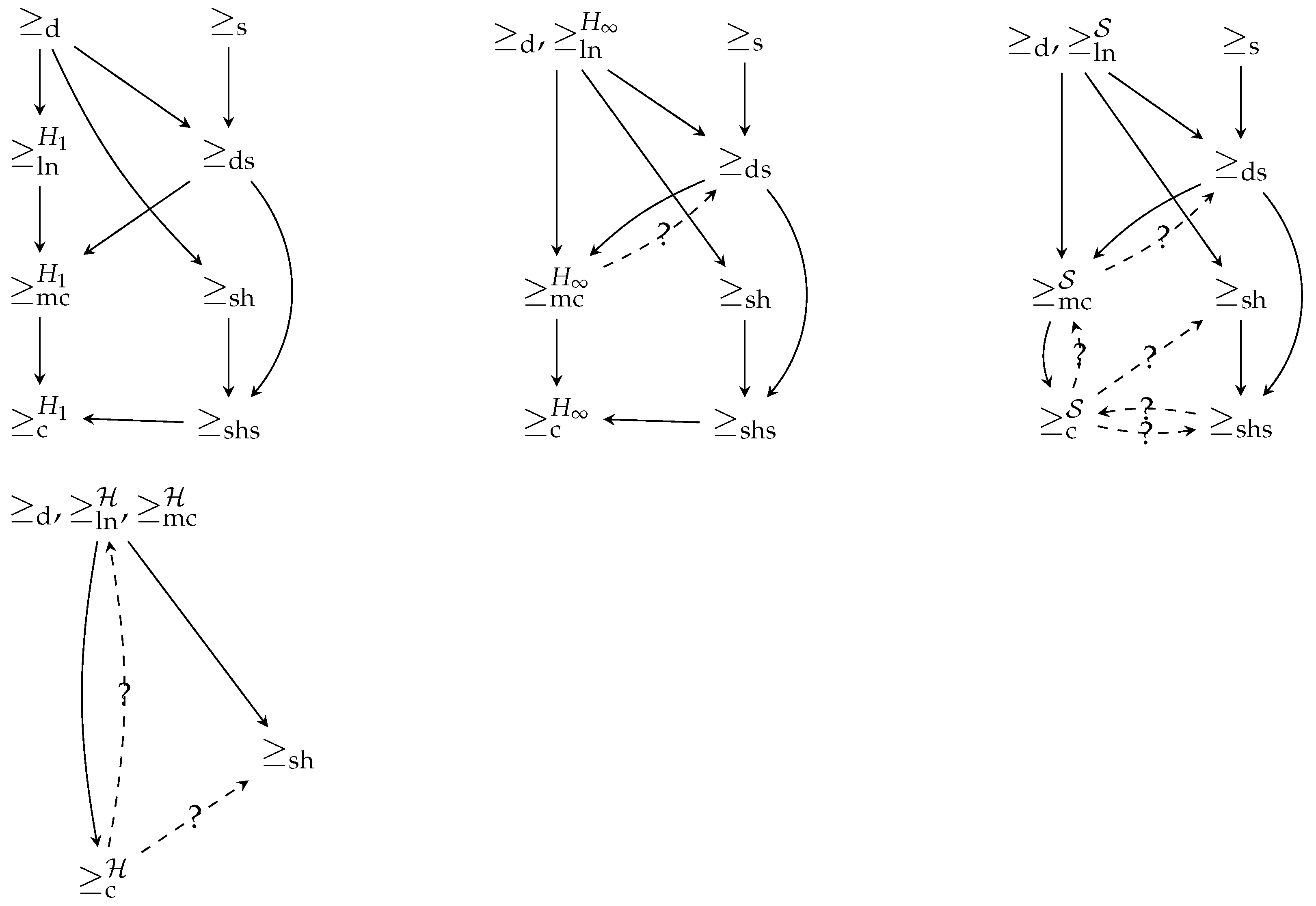
5. Relations between Preorders for Channel-Supermodular Entropies

Throughout this section, let $K_1:\mathcal{X}\to \mathcal{Y}$ and $K_2:\mathcal{X}\to \mathcal{Z}$. First, note that Proposition 1 and Theorem 2 are still meaningful under $\mathcal{S}$. The next proposition summarizes the relationship between $\left({\ge }_{\mathrm{ds}}\right)$ and the other preorders.

Proposition 5.

1. 

$K_1{\ge }_{\mathrm{d}}{K}_2\Rightarrow K_1{\ge }_{\mathrm{ds}}{K}_2$ and $K_1{\ge }_{\mathrm{s}}{K}_2\Rightarrow K_1{\ge }_{\mathrm{ds}}{K}_2$,

2. 

$K_1{\ge }_{\mathrm{ds}}{K}_2\nRightarrow K_1{\ge }_{\mathrm{d}}{K}_2$,

3. 

$K_1{\ge }_{\mathrm{ds}}{K}_2\nRightarrow K_1{\ge }_{\mathrm{s}}{K}_2$,

4. 

$K_1{\ge }_{\mathrm{ds}}{K}_2\nRightarrow K_1{\ge }_{\ln }^{\mathcal{S}}{K}_2$,

5. 

$K_1{\ge }_{\ln }^{\mathcal{S}}{K}_2\Rightarrow K_1{\ge }_{\mathrm{ds}}{K}_2$,

7. 

$K_1{\ge }_{\ln }^{H_1}{K}_2\nRightarrow K_1{\ge }_{\mathrm{ds}}{K}_2$,

8. 

$K_1{\ge }_{\mathrm{ds}}{K}_2\Rightarrow K_1{\ge }_{\mathrm{mc}}^{\mathcal{S}}{K}_2$,

8. 

$K_1{\ge }_{\mathrm{ds}}{K}_2\nRightarrow K_1{\ge }_{\mathrm{sh}}{K}_2$,

9. 

$K_1{\ge }_{\mathrm{sh}}{K}_2\nRightarrow K_1{\ge }_{\mathrm{ds}}{K}_2$.

Proof. 

See Appendix B.    □

Proposition 5.7 can be used to decide whether $K_1{\ge }_{\mathrm{mc}}^H{K}_2$, for $H\in \mathcal{S}$, by only using structural properties of the channel. Consider, for example, the following channels $K_1$, $K_2$.

$$\left(\begin{array}{ccc}\raisebox{1ex}{$1$}\!\left/ \!\raisebox{-1ex}{$2$}\right.& 0& \raisebox{1ex}{$1$}\!\left/ \!\raisebox{-1ex}{$2$}\right.\\ 0& \raisebox{1ex}{$1$}\!\left/ \!\raisebox{-1ex}{$2$}\right.& \raisebox{1ex}{$1$}\!\left/ \!\raisebox{-1ex}{$2$}\right.\\ \raisebox{1ex}{$1$}\!\left/ \!\raisebox{-1ex}{$2$}\right.& \raisebox{1ex}{$1$}\!\left/ \!\raisebox{-1ex}{$2$}\right.& 0\end{array}\right)\left(\begin{array}{cc}\raisebox{1ex}{$1$}\!\left/ \!\raisebox{-1ex}{$4$}\right.& \raisebox{1ex}{$3$}\!\left/ \!\raisebox{-1ex}{$4$}\right.\\ \raisebox{1ex}{$1$}\!\left/ \!\raisebox{-1ex}{$4$}\right.& \raisebox{1ex}{$3$}\!\left/ \!\raisebox{-1ex}{$4$}\right.\\ \raisebox{1ex}{$3$}\!\left/ \!\raisebox{-1ex}{$5$}\right.& \raisebox{1ex}{$2$}\!\left/ \!\raisebox{-1ex}{$5$}\right.\end{array}\right).$$

In [19], the authors claimed to have no proof that $K_1{\ge }_{\mathrm{mc}}^{H_1}{K}_2$. By Proposition 5 (7), $K_1{\ge }_{\mathrm{mc}}^{H_1}{K}_2$ can be proven as follows:

$$\left(\begin{array}{ccc}\raisebox{1ex}{$1$}\!\left/ \!\raisebox{-1ex}{$2$}\right.& 0& \raisebox{1ex}{$1$}\!\left/ \!\raisebox{-1ex}{$2$}\right.\\ 0& \raisebox{1ex}{$1$}\!\left/ \!\raisebox{-1ex}{$2$}\right.& \raisebox{1ex}{$1$}\!\left/ \!\raisebox{-1ex}{$2$}\right.\\ \raisebox{1ex}{$1$}\!\left/ \!\raisebox{-1ex}{$2$}\right.& \raisebox{1ex}{$1$}\!\left/ \!\raisebox{-1ex}{$2$}\right.& 0\end{array}\right){\ge }_{\mathrm{s}}\left(\begin{array}{ccc}\raisebox{1ex}{$1$}\!\left/ \!\raisebox{-1ex}{$2$}\right.& 0& \raisebox{1ex}{$1$}\!\left/ \!\raisebox{-1ex}{$2$}\right.\\ \raisebox{1ex}{$1$}\!\left/ \!\raisebox{-1ex}{$2$}\right.& 0& \raisebox{1ex}{$1$}\!\left/ \!\raisebox{-1ex}{$2$}\right.\\ \raisebox{1ex}{$1$}\!\left/ \!\raisebox{-1ex}{$2$}\right.& \raisebox{1ex}{$1$}\!\left/ \!\raisebox{-1ex}{$2$}\right.& 0\end{array}\right){\ge }_{\mathrm{d}}\left(\begin{array}{cc}\raisebox{1ex}{$1$}\!\left/ \!\raisebox{-1ex}{$4$}\right.& \raisebox{1ex}{$3$}\!\left/ \!\raisebox{-1ex}{$4$}\right.\\ \raisebox{1ex}{$1$}\!\left/ \!\raisebox{-1ex}{$4$}\right.& \raisebox{1ex}{$3$}\!\left/ \!\raisebox{-1ex}{$4$}\right.\\ \raisebox{1ex}{$3$}\!\left/ \!\raisebox{-1ex}{$5$}\right.& \raisebox{1ex}{$2$}\!\left/ \!\raisebox{-1ex}{$5$}\right.\end{array}\right).$$

Notice that if $\mathcal{H}$ is substituted for $\mathcal{S}$, Theorem 3 does not hold:

Proposition 6.

$K_1{\ge }_{\mathrm{mc}}^{\mathcal{S}}{K}_2\nRightarrow K_1{\ge }_{\mathrm{d}}{K}_2$ and $K_1{\ge }_{\mathrm{mc}}^{\mathcal{S}}{K}_2\nRightarrow K_1{\ge }_{\ln }^{\mathcal{S}}{K}_2$.

Proof. 

From Proposition 5 (2), there are channels $K_1$,$K_2$ such that $K_1{\ge }_{\mathrm{ds}}{K}_2$ and $K_1{\ngeqq }_{\mathrm{d}}{K}_2$. For such channels, Proposition 5 (7) implies $K_1{\ge }_{\mathrm{mc}}^{\mathcal{S}}{K}_2$, and the first result follows. The second result then follows by noting that Proposition 1 and Theorem 2 imply $K_1{\ge }_{\ln }^{\mathcal{S}}{K}_2\iff K_1{\ge }_{\mathrm{d}}{K}_2$.    □

Proposition 7.

$K_1{\ge }_{\mathrm{mc}}^{\mathcal{S}}{K}_2\nRightarrow K_1{\ge }_{\mathrm{sh}}{K}_2$.

Results on Channel Capacity

In [1], Shannon proved that $K_1{\ge }_{\mathrm{sh}}{K}_2\Rightarrow K_1{\ge }_{\mathrm{c}}^{H_1}{K}_2$. We can use Theorem 4 to prove similar results for the preorder ${\ge }_{\mathrm{shs}}$, which is an extension of ${\ge }_{\mathrm{sh}}$ with ${\ge }_{\mathrm{s}}$.

Definition 10.

$K_1{\ge }_{\mathrm{shs}}{K}_2$ if there are channels $W_1,\dots ,W_n$ such that $K_1{\ge }_0{W}_1{\ge }_1\dots {\ge }_{\mathrm{n}-1}{W}_n{\ge }_{\mathrm{n}}{K}_2$ where each ${\ge }_{\mathrm{i}}$ stands for ${\ge }_{\mathrm{sh}}$ or ${\ge }_{\mathrm{s}}$.

We have:

Proposition 8.

For all channels $K_1,K_2$,

1. 

$K_1{\ge }_{\mathrm{sh}}{K}_2\Rightarrow K_1{\ge }_{\mathrm{shs}}{K}_2$,

2. 

$K_1{\ge }_{\mathrm{ds}}{K}_2\Rightarrow K_1{\ge }_{\mathrm{shs}}{K}_2$,

3. 

$K_1{\ge }_{\mathrm{shs}}{K}_2\nRightarrow K_1{\ge }_{\mathrm{s}}{K}_2$,

4. 

$K_1{\ge }_{\mathrm{shs}}{K}_2\nRightarrow K_1{\ge }_{\mathrm{sh}}{K}_2$.

Proof. 

(1) and (2) follow immediately from the definitions of ${\ge }_{\mathrm{ds}}$ and ${\ge }_{\mathrm{shs}}$, and from observing that ${\ge }_{\mathrm{d}}\Rightarrow {\ge }_{\mathrm{sh}}$. (3) and (4) follow from (2) and Propositions 5 (3) and 5 (8).    □

In the remainder of this section, we prove that $K_1{\ge }_{\mathrm{shs}}{K}_2$ is a sufficient condition for establishing that both the Shannon and min-capacity of $K_1$ are at least as large as that of $K_2$.

Lemma 1.

Let $H\in \mathcal{S}$. If $K_1{\ge }_{\mathrm{sh}}{K}_2\Rightarrow K_1{\ge }_{\mathrm{c}}^H{K}_2$, then $K_1{\ge }_{\mathrm{shs}}{K}_2\Rightarrow K_1{\ge }_{\mathrm{c}}^H{K}_2$.

Proof. 

Let $H\in \mathcal{S}$. From Propositions 1, 5 (1), and 5 (7), $K_1{\ge }_{\mathrm{s}}{K}_2\Rightarrow K_1{\ge }_{\mathrm{c}}^H{K}_2$. The result then follows from Definition 10.    □

Proposition 9.

1. 

$K_1{\ge }_{\mathrm{shs}}{K}_2\Rightarrow K_1{\ge }_{\mathrm{c}}^{H_1}{K}_2$,

2. 

$K_1{\ge }_{\mathrm{shs}}{K}_2\Rightarrow K_1{\ge }_{\mathrm{c}}^{H_{\infty }}{K}_2$,

3. 

$K_1{\ge }_{\mathrm{c}}^{H_1}{K}_2\nRightarrow K_1{\ge }_{\mathrm{shs}}{K}_2$ and $K_1{\ge }_{\mathrm{c}}^{H_{\infty }}{K}_2\nRightarrow K_1{\ge }_{\mathrm{shs}}{K}_2$.

Proof. 

See Appendix B.    □

Figure 1 summarizes the implications between orderings. As can be seen, there are some open questions that need to be established, designated by dotted lines with a question mark. Note that the absence of an arrow means that the implication is known to be false.

6. Channel Design

Core-concavity was originally introduced in [51] in the context of universally optimal channel design—that is, the problem of finding, given some operational constraints, a channel leaking the minimum amount of confidential information (optimality), for all entropy-based measures of leakage (universality). This section shows how core-concavity and channel-supermodularity can be used in this context.

If X and Y are the input and output of a channel and H is a core-concave entropy, then the leakage about X through Y as measured by H is defined to be the H-mutual information $I_H(X;Y)$, as in Definition 3.

The concept of leakage is relevant in security/privacy contexts where X is some confidential data, K is modelling a system (e.g., a cryptographic computation or a database query system), and Y some observable generated by the system (e.g., the computation time or the result of a statistical query). Different H corresponds to different attackers’ models, and universal channel solutions identify countermeasures to leakage which are robust with regard to all attackers in that universe.

Minimizing leakage of sensitive information is usually a desirable goal. However, when designing systems, it is often the case that some leakage is unavoidable. With that in mind, some recent works in QIF aimed at obtaining channels that leak the least amount of information subject to some operational constraints [13,28,29]. From Definition 3, the problem can be rephrased as finding the channel which, subject to some operational constraints, maximizes $H(X|Y)$ — or, as $\eta$ is increasing, maximizes ${\sum }_{y}p\left(y\right)F(X|y)$. In a recent work [29], which considered a generalizing framework for these operational constraints, it was shown that this problem can be solved by convex optimization techniques, for a given core-concave H. However, it was also proven that the solution to the problem is in general not universal—that is, the optimal channel given a set of constraints may vary with the choice of H.

Despite this negative result, it was shown in [29] that some classes of problems admit a universal solution. As different entropies model different attackers, these results provide a very strong security guarantee—namely, that the optimal system in these situations is the most secure possible regardless of the attacker model. In the next few sections, we show how channel-supermodularity can be a useful tool in obtaining solutions that, while not universally optimal for all core-concave entropies, are the most secure for all symmetric entropies in $\mathcal{S}$.

6.1. Deterministic Channel Design Problem: A Universal Solution by Channel-Supermodularity

In many applications, such as repeated queries, it is either undesirable or impractical to consider a “probabilistic” system. This motivates the study of the channel design problem restricted to deterministic channels, which has been recently investigated in [13].

It was proven in [13] that, similarly to the general channel design problem, the deterministic version does not in general accept a universal solution. Moreover, the problem was also shown to be, in general, NP-hard. However, it was also proven in this work that a specific class of problems, called the deterministic complete k-hypergraph design problem, admit a solution that is optimal for all symmetric channel-supermodular entropies. This problem can be defined as follows.

Definition 11.

Let $H\in \mathcal{H}$, $k\in {\mathbb{N}}_{>0}$ and let $\mathcal{X},\mathcal{Y}$ be finite sets with $|\mathcal{Y}|\ge |\mathcal{X}|/k$

The deterministic complete k-hypergraph design problem (CKDP) is to find a channel $K:\mathcal{X}\to \mathcal{Y}$ that maximizes $H(X|Y)$, subject to the following constraints:

• $\forall x,y,K(y|x)\in \{0,1\}$, and
• $\forall y,{\sum }_{x}K(y|x)\le k$.

That is, the deterministic CKDP is the problem of finding the most secure deterministic channel, subject to the constraint that each output can only be generated by at most k inputs.

For the remainder of this section, let $k\in {\mathbb{N}}_{>0}$, and fix a distribution $p_X$ such that, without loss of generality, $p_X\left(x_i\right)\ge p_X\left(x_j\right)$ whenever $i<j$.

The greedy solution proposed by [13] is described in Algorithm 1. The algorithm is straightforward: it associates the k most likely secrets with the first observable; it then associates the k most likely secrets among the remaining secrets with the second observable, and so on. The solution for $\mathcal{X}=\{x_1,\dots ,x_8\}$ and $k=3$ is depicted in Figure 2.

Algorithm 1 Greedy algorithm for the k-complete hypergraph problem

Input: Input set $\mathcal{X}$, prior $p_X$ and integer $k\le |\mathcal{X}|$ Output: Matrix of optimal deterministic channel $K_k$

1: initialize: $K_k$ as a matrix of 0s, with $|\mathcal{X}|$ rows and $\lceil |\mathcal{X}|/k\rceil$ columns.

2: for $i\in \{1,\dots ,|\mathcal{X}|\}$do

3:    $K_k(i,\lceil i/k\rceil )=1$

4:return$K_k$

Theorem 6

([13]). Given a complete k-hypergraph channel design problem, the solution given by Algorithm 1 is optimal for any symmetric channel-supermodular entropy.

Proof. 

We reproduce the proof of this theorem from [13], as it provides an interesting application of channel-supermodularity. Let us consider the following joint matrix $J_k$ obtained by Algorithm 1 and the prior:

$$\begin{array}{c}\left(\begin{array}{cccc}{p}_1& 0& \dots & 0\\ ⋮& ⋮& & ⋮\\ p_k& 0& & ⋮\\ 0& p_{k+1}& & ⋮\\ ⋮& ⋮& & ⋮\\ ⋮& p_{2k}& & ⋮\\ ⋮& 0& & ⋮\\ ⋮& ⋮& \ddots & ⋮\\ ⋮& ⋮& & 0\\ ⋮& ⋮& & p_{mk+1}\\ ⋮& ⋮& & ⋮\\ 0& 0& \dots & p_n\end{array}\right)\end{array}$$

We now prove that any matrix J satisfying the constraints can be transformed into $J_k$ by a sequence of steps each increasing (or keeping equal) any supermodular entropy. Each step consists of the following three sub-steps:

• Select two columns $c_i,c_j$ and align the non-zero coefficients in $c_i,c_j$;
• Perform $\wedge ,\vee$ operations on the aligned columns and replace $c_i,c_j$ with $c_i\vee c_j,c_i\wedge c_j$;
• Disalign the two columns $c_i\vee c_j,c_i\wedge c_j$.

The following example illustrates one step (i.e., the three sub-steps above):

$$\left(\begin{array}{ccc}0& 0.4& 0\\ 0& 0& 0.3\\ 0& 0.15& 0\\ 0& 0& 0.1\\ 0.05& 0& 0\end{array}\right)\stackrel{=}{\to }\left(\begin{array}{ccc}0& 0.4& 0.1\\ 0& 0.15& 0.3\\ 0& 0& 0\\ 0& 0& 0\\ 0.05& 0& 0\end{array}\right)\stackrel{\le }{\to }\left(\begin{array}{ccc}0& 0.4& 0.1\\ 0& 0.3& 0.15\\ 0& 0& 0\\ 0& 0& 0\\ 0.05& 0& 0\end{array}\right)\stackrel{=}{\to }\left(\begin{array}{ccc}0& 0.4& 0\\ 0& 0.3& 0\\ 0& 0& 0.15\\ 0& 0& 0.1\\ 0.05& 0& 0\end{array}\right)$$

from left to right we have:

• selected $c_2,c_3$, which are the two columns containing the two most likely priors (i.e., 0.4 and 0.3) and aligned $c_2,c_3$ so that 0.4, 0.3 appear in different rows;
• replaced $c_2,c_3$ with $c_2\vee c_3,c_2\wedge c_3$;
• disaligned columns 2 and 3, that is, position values in $c_2\vee c_3,c_2\wedge c_3$, so that each row has the same probability it had before the step.

Notice that aligning (and disaligning) is a permutation of a column; hence, they do not change the value of the posterior of symmetric channel-supermodular entropies because $G_F\left(c_i\right)=G_F\left(c_i^{\prime }\right)$ for any permutation $c_i^{\prime }$ of the column $c_i$.

Next, for the remaining sub-step, where we replace $c_i,c_j$ with $c_i\vee c_j,c_i\wedge c_j$, by supermodularity of G we have $G_F\left(c_i\right)+G_F\left(c_j\right)\le G_F(c_i\vee c_j)+G_F(c_i\wedge c_j)$; hence, that sub-step increases (or keeps equal) the posterior entropy. Notice also that the matrix at the end of the step has in each row the same probabilities as it had before that step; hence, it is still a joint matrix that respects the complete k-hypergraph constraints for the same prior.

The selection and alignment of columns is as follows: at the initial step select $c_i$ such that $c_i$ contains the first r elements with the highest probabilities, say $p_1,\dots ,p_r$; if $r<k$, then select $c_j$ as the column containing $p_{r+1}$; align $c_i,c_j$ so that $p_{r+1}$ is not on the same row as any of the $p_1,\dots ,p_r$ (and $c_i\vee c_j$ has no more than k non-zero terms). Then, $c_i\vee c_j$ will contain $p_1,\dots ,p_{r+1}$. Repeat until $r=k$. Then repeat the process considering the probabilities $p_{k+1},\dots ,p_n$.

By repeating these steps, we will reach a matrix $J^{\prime }$ with columns $c_1^{\prime },\dots ,c_n^{\prime }$ such that each element of column $c_i^{\prime }$ has higher probability than all elements of column $c_{i+1}^{\prime }$. This is exactly the solution given by the greedy algorithm (modulo column permutations), that is, $J^{\prime }=J_k$. □

If H is not channel-supermodular, the greedy solution may not be optimal. Consider, for example, the Hayashi–Rényi entropies, which are not channel-supermodular. Let $\mathcal{X}=\{x_1,\dots ,x_4\}$, $p_X=(0.3,0.3,0.2,0.2)$ and $k=3$, and consider the channels $K_1,K_2$ with outputs $Y_1,Y_2$ below.

$$\begin{array}{|ccc|}\hline K_1& y_1& y_2\\ x_1& 1& 0\\ x_2& 1& 0\\ x_3& 1& 0\\ x_4& 0& 1\\ \hline\end{array}\begin{array}{|ccc|}\hline K_2& y_1& y_2\\ x_1& 1& 0\\ x_2& 1& 0\\ x_3& 0& 1\\ x_4& 0& 1\\ \hline\end{array}$$

Then, $K_1$ is the greedy solution. However, for Hayashi–Rényi entropies, the following limit holds [52]:

$$\underset{\alpha \to \infty }{lim}{H}_{\alpha }^{\prime }(X|Y)=-log\left(\underset{y\in \sim \approxeq \parallel \left(Y\right),x\in \mathcal{X}}{max}{p}_{X|y}\left(x\right)\right),$$

Therefore,

$$\underset{\alpha \to \infty }{lim}{H}_{\alpha }^{\prime }(X|Y_1)=0,$$

whereas

$$\underset{\alpha \to \infty }{lim}{H}_{\alpha }^{\prime }(X|Y_2)=1.$$

Thus, $H_{\alpha }^{\prime }(X|Y_1)<H_{\alpha }^{\prime }(X|Y_2)$ for large enough $\alpha$, and the greedy solution is not optimal.

Another example of core-concave functions for which Algorithm 1 is not optimal is provided by “partition” entropies. For example, if B is a partition of the possible values of X then

$$H_B\left(X\right)=-log\underset{S\in B}{max}\sum _{x\in S}{p}_X\left(x\right)$$

is a core-concave entropy which is not channel-supermodular.

6.2. An Application to Query Anonymity

Let us consider the following anonymity mechanism problem: we want to design an anonymity mechanism where in order to conceal a secret query from an eavesdropper, the user sends to a server a set of k queries which includes the secret query. Then, once received from the server the response to all the k queries, the user retrieves the response to the secret query. In our setting, this corresponds to each observable having a pre-image of size exactly k.

As an illustrative example consider a Twitter user who wants to visit some other Twitter user page but wants to keep this query secret. To solve this problem, he decides to use the following protocol: whenever he visits the desired user page, he also sends $k-1$ other queries to the pages of other Twitter users. Suppose further that this user frequently visits this user’s page, meaning that a random choice of the other queries is not a wise strategy, since multiple observations would end up revealing more and more information about the query, eventually completely revealing the secret query. The problem is then: which set of k Twitter pages will leak the least information about the user secret query?

We assume the attacker has no background information about the user, and hence we set the probability of a Twitter query for that user as the probability that a general member of the public requests that Twitter page (a good proxy to this measure can be derived by the number of followers of that Twitter page). Let n be the number of possible queries (i.e., the input set). Considering the scenario that n is divisible by k, we can use Algorithm 1 to solve this problem.

Notice that for n secrets, there are $n!{(\frac{n}{k}!)}^{-1}{(k!)}^{-\frac{n}{k}}$ possible ways to satisfy these anonymity constraints. For example, there are about $7\times {10}^{85}$ possible solutions when $n=100$ and $k=10$, and about $4\times {10}^{19,704}$ for $n=$ 10,000 and $k=100$. We will now compare the greedy algorithm in Section 6 against other possible anonymity solutions, and we will measure the goodness of the solutions using min and Shannon posterior entropies. Let us consider the three anonymity solutions below:

• the solution from the greedy algorithm (Algorithm 1) (i.e., pick the $k-1$ queries closest in probability to the real query);
• a random solution (i.e., pick k random queries);
• a non-optimal solution where the secrets with the highest probabilities, instead of being grouped in the first bin, are distributed in the other bins.

For example, for 6 secrets and $k=2$, the greedy solution would be $\{\{x_1,x_2\},$$\{x_3,x_4\},$$\{x_5,x_6\}\}$, whereas the non-optimal solution (3) would be $\{\{x_1,x_4\},$$\{x_2,x_5\},$$\{x_3,x_6\}\}$.

The difference between these solutions can be very substantial. Figure 3 shows the values when the distribution over the input set is a binomial distribution, with parameter $p=0.5$: in this scenario, supposing that there is a universe of 350 Twitter pages and that the user sends 19 queries selected using the greedy algorithm, the probability of an attacker guessing the secret query correctly would be over 7 times smaller than if the user had opted instead for the non-optimal solution (using $2^{-H_{\infty }(X|Y)}$ as the conversion formula from posterior min entropy to probability of guessing). In fact, it is easy to define an input probability distribution such that the leakage gap between the non-optimal solution and the optimal solution given by the greedy algorithm is arbitrarily large.

Note that, by Theorem 6, the greedy solution is in fact optimal for all channel-supermodular entropies. Hence, the user knows that the greedy solution is optimal against an attacker trying to guess his secret query in a fixed number of guesses, or using guesswork or guessing using a twenty-questions-style guesswork (reflecting Shannon entropy), and so on.

6.3. Query Anonymity for Related Secrets

Consider the scenario where a user who wants to query the Twitter page of some political commentators is at the same time interested in hiding his own political affiliation, which could be leaked by his queries. In this scenario, the solution from Algorithm 1 might be sub-optimal. To see this, suppose that the k queries in the real query’s cover end up being all affiliated to the same party. This would thus reveal the user’s political party to the attacker with certainty even though the real intended query is still uncertain. This is not a contradiction to the optimality of the algorithm. As such, an adversary would be better modeled by a partition entropy—with political commentators (the queried users) grouped by party affiliation—and, as established in Proposition 3, this type of entropy is not channel-supermodular in general.

Motivated by this scenario, we now give an optimal solution for all channel supermodular entropies (even if not symmetric) to deal with this kind of problem. Suppose there are k political parties, and l commentators aligned with each party. Suppose, further, that the user is affiliated to one of the parties, and would like to check the profiles of his party’s commentators without revealing his own affiliation.

To achieve this aim, the user decides to group the political commentators in covers of size k, each cover containing exactly one commentator from each party, and then proceed to use these covers similarly to the mechanism described in Section 6.2, by querying the entire cover (fetching the pages of all the commentators in the cover). The question is: what is the set of covers that reveal the least amount of information about the user’s political affiliation?

Let $\mathcal{X}=\{P_1,\dots P_k\}$ be the set of parties, $\mathcal{Y}=\{c_1^1,\dots ,c_1^l,c_2^1,\dots ,c_2^l,\dots ,\dots ,c_k^1,\dots ,c_k^l\}$ be the set of commentators, wherein $c_i^j$ is the jth commentator of the ith party, and let $\mathcal{Z}\subset 2^{\mathcal{Y}}$ be the set of covers. Let $K:\mathcal{X}\to \mathcal{Y}$ be the channel giving the conditional probability of a user choosing to query a commentator given the user’s party inclination. We assume that the user only chooses commentators that share the same affiliation as his, that is, $K(c_j^i|P_m)=0$ whenever $j\ne m$. For simplicity, we assume that the commentators are organized decreasingly with regard to this probability—that is,

$$K(c_j^i|P_j)\ge K(c_j^m|P_j)\mathrm{whenever}m>i.$$

(6)

We claim that the optimal mechanism, for all channel-supermodular entropies (with regards to the political parties, not the commentators), is to group the most popular commentators for each party in the first cover, then the second-most popular commentators for each party on the second, and so on. That is, the covers would be: $\{\{c_1^1,c_2^1,\dots ,c_k^1\}$, $\{c_1^2,c_2^2,\dots ,c_k^2\}$, …, $\{c_1^l,c_2^l,\dots ,c_k^l\}\}$.

Let $R:\mathcal{Y}\to \mathcal{Z}$ be the channel mapping each commentator to their cover, modelling the optimal solution described above. The matrix of this channel can be seen as a vertical concatenation of identity matrices:

$$\begin{array}{|ccccc|}\hline R& Cove{r}_1& Cove{r}_2& \dots & Cove{r}_l\\ c_1^1& 1& 0& \dots & 0\\ c_1^2& 0& 1& \dots & 0\\ ⋮& ⋮& ⋮& \ddots & ⋮\\ c_1^l& 0& 0& \dots & 1\\ ⋮& & ⋮& & \\ ⋮& & ⋮& & \\ c_k^1& 1& 0& \dots & 0\\ c_k^2& 0& 1& \dots & 0\\ \dots & \dots & \dots & \ddots & \dots \\ c_k^1& 0& 0& \dots & 1\\ \hline\end{array}\begin{array}{|ccccc|}\hline KR& Cove{r}_1& Cove{r}_2& \dots & Cove{r}_l\\ P_1& K(c_1^1|P_1)& K(c_1^2|P_1)& \dots & K(c_1^l|P_1)\\ P_2& K(c_2^1|P_2)& K(c_2^2|P_2)& \dots & K(c_2^l|P_2)\\ ⋮& ⋮& ⋮& & ⋮\\ P_k& K(c_k^1|P_k)& K(c_k^2|P_k)& \dots & K(c_k^l|P_k)\\ \hline\end{array}$$

(7)

The channel $KR:\mathcal{X}\to \mathcal{Z}$ above is then obtained by postprocessing K by R.

The claim of optimally can be more formally stated as follows: given any channel-supermodular H, any distribution $p_X$ over the parties, and any other deterministic covering $R^{\prime }:\mathcal{Y}\to {\mathcal{Z}}^{\prime }$ in which there is exactly one commentator from each party per cover, the resulting channel $K{R}^{\prime }$ will never leak less information than the channel $KR$ in (7). That is,

$$H(X|Z)\ge H(X|Z^{\prime }).$$

The proof that the covering R above is indeed optimal for all channel-supermodular entropies is similar to the proof of Theorem 6, but even simpler. Suppose the channel $R^{\prime }:\mathcal{Y}\to \mathcal{Z}$ is any covering that satisfies the restriction that each cover has exactly one commentator from each party. Now, consider the channel $K{R}^{\prime }$, and proceed as follows: first, do the Join-Meet operation of the first column with all the other columns (that is, obtaining the channel ${\diamond }_{1,l}{\diamond }_{1,l-1}\dots {\diamond }_{1,2}\left(K{R}^{\prime }\right)$ ). Now, disregarding the first column, the process is repeated for the second column with all the remaining ones. It is easy to see that the resulting channel will be exactly $KR$ in (7).

As an example, let $k=3$, $l=3$, and suppose the non-zero values of K are:

$$\begin{array}{c}\hfill K(c_1^1|P_1)=0.5,K(c_1^2|P_1)=0.3,K(c_1^3|P_1)=0.2\\ \hfill K(c_2^1|P_2)=0.6,K(c_2^2|P_2)=0.3,K(c_2^3|P_2)=0.1\\ \hfill K(c_3^1|P_3)=0.5,K(c_3^2|P_3)=0.4,K(c_3^3|P_3)=0.1\end{array}$$

and suppose that the covers that are defined by $R^{\prime }$ are $\{c_1^2,c_2^1,c_3^2\}$, $\{c_1^1,c_2^3,c_3^1\}$, and $\{c_1^3,c_2^2,c_3^3\}$. We have

$$\begin{array}{|cccc|}\hline K{R}^{\prime }& Cove{r}_1& Cove{r}_2& Cove{r}_3\\ P_1& 0.3& 0.5& 0.2\\ P_2& 0.6& 0.1& 0.3\\ P_3& 0.4& 0.5& 0.1\\ \hline\end{array}$$

By doing the Join-Meet operations on the first column with the others, we obtain

$$\begin{array}{|cccc|}\hline {\diamond }_{1,3}{\diamond }_{1,2}\left(K{R}^{\prime }\right)& Cove{r}_1& Cove{r}_2& Cove{r}_3\\ P_1& 0.5& 0.3& 0.2\\ P_2& 0.6& 0.1& 0.3\\ P_3& 0.5& 0.4& 0.1\\ \hline\end{array}$$

Finally, by doing the Join-Meet of the second column with the remaining one, we have

$$\begin{array}{|cccc|}\hline {\diamond }_{2,3}{\diamond }_{1,3}{\diamond }_{1,2}\left(K{R}^{\prime }\right)& Cove{r}_1& Cove{r}_2& Cove{r}_3\\ P_1& 0.5& 0.3& 0.2\\ P_2& 0.6& 0.3& 0.1\\ P_3& 0.5& 0.4& 0.1\\ \hline\end{array}$$

which is exactly the optimal solution given by (7).

7. Conclusions

In this work, we introduced the notion of channel-supermodular entropies, as a subset of core-concave entropies, which include guessing and Arimoto–Rényi entropies. We demonstrated that, for this new classification of entropies, the Join-Meet operator on channel columns decreases the H-mutual information. This property prompted us to define structural preorders of channels (${\ge }_{\mathrm{ds}},{\ge }_{\mathrm{sds}}$), providing novel sufficient conditions for establishing whether two channels are in the H-more capable any channel-supermodular H or in the $(H_1,H_{\infty })$-capacity ordering. Moreover, this work establishes some relationships of these new structural preorders with other existing preorders from the literature.

As an example application, we used channel-supermodularity to prove an optimality result of a greedy query anonymization algorithm.

It is our belief that the connection between supermodular functions and some commonly used entropy measures, made in Section 3.1, will prove useful for posterior investigations in information theory (for example, given the vast literature of supermodular functions over Euclidean space [50] (Chapter 6.D) and [49]). Further directions of work include investigating other useful properties of channel-supermodular entropies, and further applications of channel-supermodularity to anonymity.

References

1. Shannon, C.E. A note on a partial ordering for communication channels. Inf. Control 1958, 1, 390–397. [Google Scholar] [CrossRef] [Green Version]
2. El Gamal, A.A. The capacity of a class of broadcast channels. IEEE Trans. Inf. Theory 1979, 25, 166–169. [Google Scholar] [CrossRef]
3. Korner, J.; Marton, K. Comparison of two noisy channels. Coll. Math. Soc. J. Bolyai 1977, 16, 411–423. [Google Scholar]
4. Clark, D.; Hunt, S.; Malacaria, P. Quantitative Information Flow, Relations and Polymorphic Types. J. Log. Comput. 2005, 15, 181–199. [Google Scholar] [CrossRef]
5. Smith, G. On the Foundations of Quantitative Information Flow. In Proceedings of the 12th International Conference on Foundations of Software Science and Computational Structures (FOSSACS), York, UK, 22–29 March 2009; Springer: Berlin/Heidelberg, Germany, 2009; Volume 5504, pp. 288–302. [Google Scholar]
6. Cohen, J.; Kempermann, J.H.B.; Zbaganu, G. Comparisons of Stochastic Matrices with Applications in Information Theory, Statistics, Economics and Population; Springer Science & Business Media: Berlin/Heidelberg, Germany, 1998. [Google Scholar]
7. Américo, A.; Malacaria, P.; Khouzani, A.M. Channel Ordering and Supermodularity. In Proceedings of the 2019 IEEE Information Theory Workshop (ITW) (IEEE ITW 2019), Visby, Sweden, 25–28 August 2019. [Google Scholar]
8. Cover, T.M. Broadcast channels. IEEE Trans. Inf. Theory 1972, 18, 2–14. [Google Scholar] [CrossRef] [Green Version]
9. Pasareanu, C.S.; Phan, Q.; Malacaria, P. Multi-run Side-Channel Analysis Using Symbolic Execution and Max-SMT. In Proceedings of the IEEE 29th Computer Security Foundations Symposium, CSF 2016, Lisbon, Portugal, 27 June–1 July 2016; pp. 387–400. [Google Scholar] [CrossRef]
10. Heusser, J.; Malacaria, P. Quantifying information leaks in software. In Proceedings of the Twenty-Sixth Annual Computer Security Applications Conference, ACSAC 2010, Austin, TX, USA, 6–10 December 2010; pp. 261–269. [Google Scholar] [CrossRef]
11. Gong, X.; Kiyavash, N. Quantifying the information leakage in timing side channels in deterministic work-conserving schedulers. IEEE/ACM Trans. Netw. 2016, 24, 1841–1852. [Google Scholar] [CrossRef] [Green Version]
12. Köpf, B.; Smith, G. Vulnerability Bounds and Leakage Resilience of Blinded Cryptography under Timing Attacks. In Proceedings of the 2010 23rd IEEE Computer Security Foundations Symposium, Edinburgh, UK, 17–19 July 2010; pp. 44–56. [Google Scholar]
13. Américo, A.; Khouzani, M.; Malacaria, P. Deterministic Channel Design for Minimum Leakage. In Proceedings of the IEEE 32nd Computer Security Foundations Symposium (CSF), Hoboken, NJ, USA, 25–28 June 2019; pp. 428–441. [Google Scholar] [CrossRef]
14. Bergmans, P. Random coding theorem for broadcast channels with degraded components. IEEE Trans. Inf. Theory 1973, 19, 197–207. [Google Scholar] [CrossRef]
15. Bergmans, P. A simple converse for broadcast channels with additive white Gaussian noise (Corresp.). IEEE Trans. Inf. Theory 1974, 20, 279–280. [Google Scholar] [CrossRef]
16. Gallager, R.G. Capacity and coding for degraded broadcast channels. Probl. Peredachi Informatsii 1974, 10, 3–14. [Google Scholar]
17. Smith, G. Recent Developments in Quantitative Information Flow (Invited Tutorial). In Proceedings of the LICS ’15 2015 30th Annual ACM/IEEE Symposium on Logic in Computer Science (LICS), Kyoto, Japan, 6–10 July 2015; IEEE Computer Society: Washington, DC, USA, 2015; pp. 23–31. [Google Scholar] [CrossRef]
18. Malacaria, P. Algebraic foundations for quantitative information flow. Math. Struct. Comput. Sci. 2015, 25, 404–428. [Google Scholar] [CrossRef] [Green Version]
19. Alvim, M.S.; Chatzikokolakis, K.; Palamidessi, C.; Smith, G. Measuring Information Leakage Using Generalized Gain Functions. In Proceedings of the IEEE 25th Computer Security Foundations Symposium (CSF), Cambridge, MA, USA, 25–27 June 2012; pp. 265–279. [Google Scholar] [CrossRef] [Green Version]
20. McIver, A.; Morgan, C.; Smith, G.; Espinoza, B.; Meinicke, L. Abstract Channels and Their Robust Information-Leakage Ordering. In Proceedings of the International Conference on Principles of Security and Trust (POST), Grenoble, France, 5–13 April 2014; Springer: Berlin/Heidelberg, Germany, 2014; Volume 8414, pp. 83–102. [Google Scholar]
21. Blackwell, D. The comparison of experiments. In Second Berkeley Symposium on Mathematical Statistics and Probability; Neyman, J., Ed.; Univ. of California Press: Berkeley, CA, USA, 1951; pp. 93–102. [Google Scholar]
22. Bordenabe, N.E.; Smith, G. Correlated Secrets in Quantitative Information Flow. In Proceedings of the 2016 IEEE 29th Computer Security Foundations Symposium (CSF), Lisbon, Portugal, 27 June–1 July 2016; pp. 93–104. [Google Scholar] [CrossRef]
23. Buscemi, F. Degradable channels, less noisy channels, and quantum statistical morphisms: An equivalence relation. Probl. Inf. Transm. 2016, 52, 201–213. [Google Scholar] [CrossRef] [Green Version]
24. Cam, L.L. Sufficiency and Approximate Sufficiency. Ann. Math. Stat. 1964, 35, 1419–1455. [Google Scholar] [CrossRef]
25. Raginsky, M. Shannon meets Blackwell and Le Cam: Channels, codes, and statistical experiments. In Proceedings of the 2011 IEEE International Symposium on Information Theory Proceedings, St. Petersburg, Russia, 31 July–5 August 2011; pp. 1220–1224. [Google Scholar] [CrossRef]
26. Zhang, Y.; Tepedelenlioğlu, C. Analytical and Numerical Characterizations of Shannon Ordering for Discrete Memoryless Channels. IEEE Trans. Inf. Theory 2014, 60, 72–83. [Google Scholar] [CrossRef] [Green Version]
27. Nasser, R. Characterizations of Two Channel Orderings: Input-Degradedness and the Shannon Ordering. IEEE Trans. Inf. Theory 2018, 64, 6759–6770. [Google Scholar] [CrossRef]
28. Khouzani, M.; Malacaria, P. Generalised Entropies and Metric-Invariant Optimal Countermeasures for Information Leakage under Symmetric Constraints. IEEE Trans. Inf. Theory 2018, 65, 888–901. [Google Scholar] [CrossRef] [Green Version]
29. Khouzani, M.; Malacaria, P. Leakage-Minimal Design: Universality, Limitations, and Applications. In Proceedings of the IEEE 30th Computer Security Foundations Symposium (CSF), Santa Barbara, CA, USA, 21–25 August 2017; pp. 305–317. [Google Scholar]
30. Khouzani, M.; Malacaria, P. Optimal Channel Design: A Game Theoretical Analysis. Entropy 2018, 20, 675. [Google Scholar] [CrossRef] [PubMed] [Green Version]
31. Ah-Fat, P.; Huth, M. Optimal Accuracy-Privacy Trade-Off for Secure Computations. IEEE Trans. Inf. Theory 2018, 65, 3165–3182. [Google Scholar] [CrossRef]
32. Köpf, B.; Basin, D.A. An information-theoretic model for adaptive side-channel attacks. In Proceedings of the 14th ACM Conference on Computer and Communications Security, Alexandria, VA, USA, 2 November–31 October 2007; pp. 286–296. [Google Scholar] [CrossRef] [Green Version]
33. Espinoza, B.; Smith, G. Min-entropy as a resource. Inf. Comp. 2013, 226, 57–75. [Google Scholar] [CrossRef]
34. Alvim, M.S.; Chatzikokolakis, K.; McIver, A.; Morgan, C.; Palamidessi, C.; Smith, G. Additive and Multiplicative Notions of Leakage, and Their Capacities. In Proceedings of the IEEE 27th Computer Security Foundations Symposium (CSF), Vienna, Austria, 19–22 July 2014; pp. 308–322. [Google Scholar] [CrossRef] [Green Version]
35. Gervais, A.; Shokri, R.; Singla, A.K.; Capkun, S.; Lenders, V. Quantifying Web-Search Privacy. In Proceedings of the 2014 ACM SIGSAC Conference on Computer and Communications Security, Scottsdale, AZ, USA, 3–7 November 2014. [Google Scholar]
36. Beigi, G.; Guo, R.; Nou, A.; Zhang, Y.; Liu, H. Protecting User Privacy: An Approach for Untraceable Web Browsing History and Unambiguous User Profiles. arXiv 2018, arXiv:cs.CR/1811.09340. [Google Scholar]
37. Rebollo-Monedero, D.; Forne, J. Optimized Query Forgery for Private Information Retrieval. IEEE Trans. Inf. Theory 2010, 56, 4631–4642. [Google Scholar] [CrossRef] [Green Version]
38. Alvim, M.S.; Chatzikokolakis, K.; McIver, A.; Morgan, C.; Palamidessi, C.; Smith, G. An axiomatization of information flow measures. Theor. Comput. Sci. 2019, 777, 32–54. [Google Scholar] [CrossRef]
39. Arimoto, S. Information-theoretical considerations on estimation problems. Inf. Control 1971, 19, 181–194. [Google Scholar] [CrossRef] [Green Version]
40. Salicru, M.; Menendez, M.; Morales, D.; Pardo, L. Asymptotic distribution of (h, Φ)-entropies. Commun. Stat.-Theory Methods 1993, 22, 2015–2031. [Google Scholar] [CrossRef]
41. Csiszár, I. Information-type measures of difference of probability distributions and indirect observation. Stud. Sci. Math. Hung. 1967, 2, 229–318. [Google Scholar]
42. Ho, S.W.; Verdú, S. Convexity/concavity of rényi entropy and α-mutual information. In Proceedings of the 2015 IEEE International Symposium on Information Theory (ISIT), Hong Kong, China, 14–19 June 2015; pp. 745–749. [Google Scholar] [CrossRef]
43. Arimoto, S. Information measures and capacity of order α for discrete memoryless channels. In Topics in Information Theory; North-Holland Publishing Company: Amsterdam, The Netherlands, 1977. [Google Scholar]
44. Massey, J.L. Guessing and entropy. In Proceedings of the IEEE Int. Symposium on Information Theory (ISIT), Trondheim, Norway, 27 June–1 July 1994; p. 204. [Google Scholar] [CrossRef]
45. Tsallis, C. Possible generalization of Boltzmann-Gibbs statistics. J. Stat. Phys. 1988, 52, 479–487. [Google Scholar] [CrossRef]
46. Sharma, B.; Mittal, D. New non-additive measures of entropy for discrete probability distributions. J. Math. Sci. 1975, 10, 28–40. [Google Scholar]
47. Hayashi, M. Exponential decreasing rate of leaked information in universal random privacy amplification. IEEE Trans. Inf. Theory 2011, 57, 3989–4001. [Google Scholar] [CrossRef] [Green Version]
48. Dahl, G. Matrix majorization. Linear Algebra Its Appl. 1999, 288, 53–73. [Google Scholar] [CrossRef] [Green Version]
49. Topkis, D.M. Supermodularity and Complementarity; Princeton University Press: Princeton, NJ, USA, 1998. [Google Scholar]
50. Marshall, A.W.; Olkin, I.; Arnold, B.C. Inequalities: Theory of Majorization and Its Applications; Mathematics in Science and Engineering; Academic Press: Cambridge, MA, USA, 1979; Volume 143. [Google Scholar]
51. Khouzani, M.H.R.; Malacaria, P. Relative Perfect Secrecy: Universally Optimal Strategies and Channel Design. In Proceedings of the IEEE 29th Computer Security Foundations Symposium, CSF 2016, Lisbon, Portugal, 27 June–1 July 2016; pp. 61–76. [Google Scholar] [CrossRef]
52. Iwamoto, M.; Shikata, J. Information Theoretic Security for Encryption Based on Conditional Rényi Entropies. In Information Theoretic Security; Padró, C., Ed.; Springer International Publishing: Cham, Switzerland, 2014; pp. 103–121. [Google Scholar]
53. Cover, T.M.; Thomas, J.A. Elements of Information Theory, 2nd ed.; John Wiley & Sons, Inc.: Hoboken, NJ, USA, 2006. [Google Scholar]
Figure 1. The four implication graphs summarize the relation between preorders. It is known that a preorder i implies a preorder j if and only if there is a path of solid arrows from i to j . Preorders that are equivalent are grouped together, and the dotted arrows represent an implication whose validity is an open question. When no path is present, the implication is known not to hold.
Entropy 24 00039 g001
Figure 2. The solution given by Algorithm 1 for k = 3 .
Entropy 24 00039 g002
Figure 3. Posterior Shannon and min-entropy for different anonymity solutions. k is n , where n is the size of the input set. For the random solution, the values in the plot are the average of 1000 samples.
Entropy 24 00039 g003