
Temporal Variation of b Value with Statistical Test in Wenchuan Area, China Prior to the 2008 Wenchuan Earthquake


Abstract
:1. Introduction
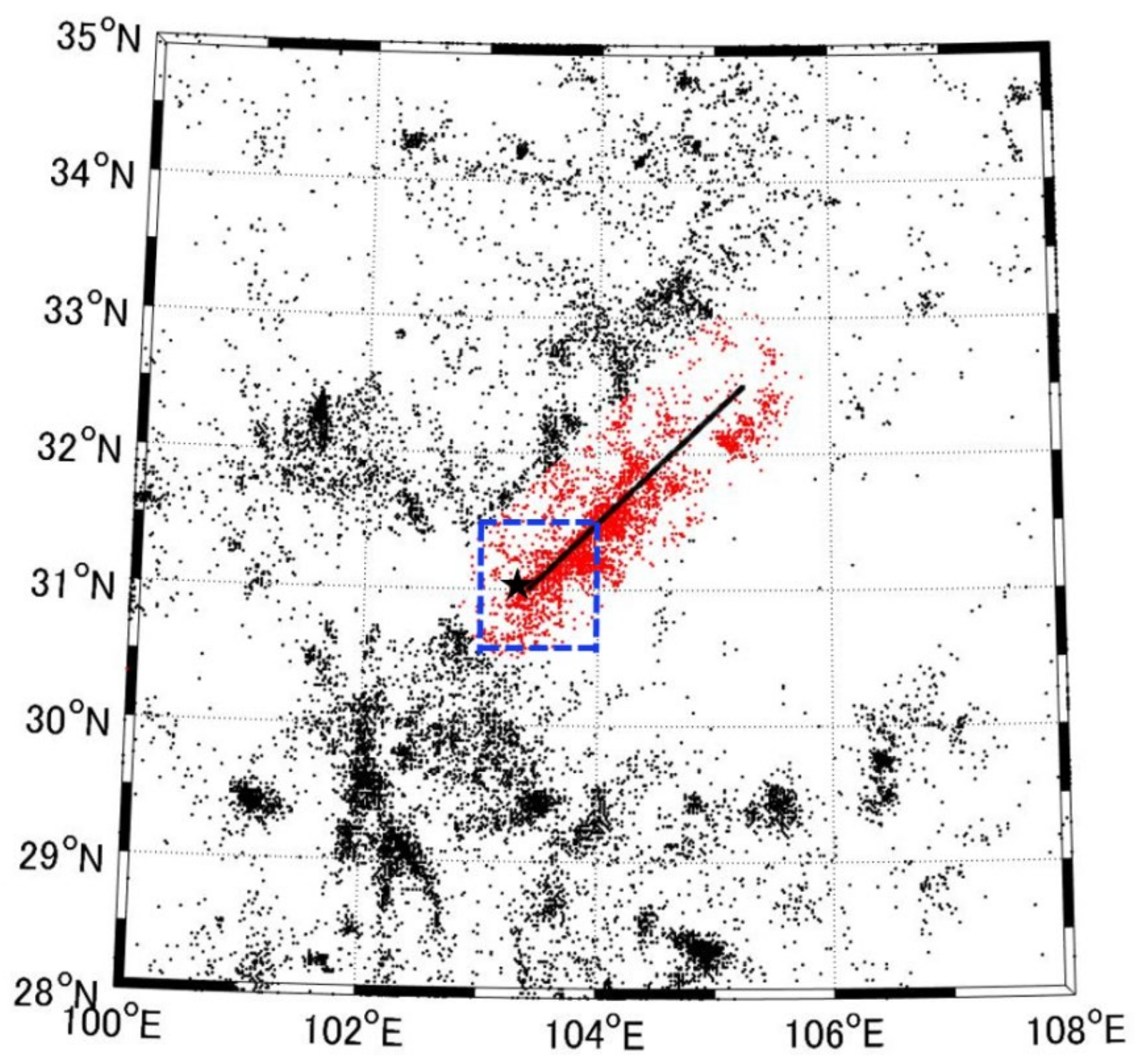
2. Data
3. Methods
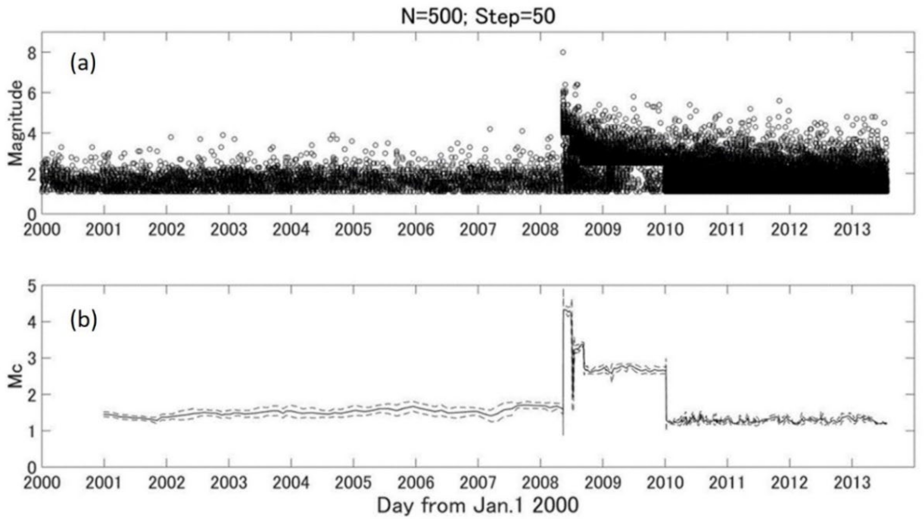
3.1. Estimation of MC
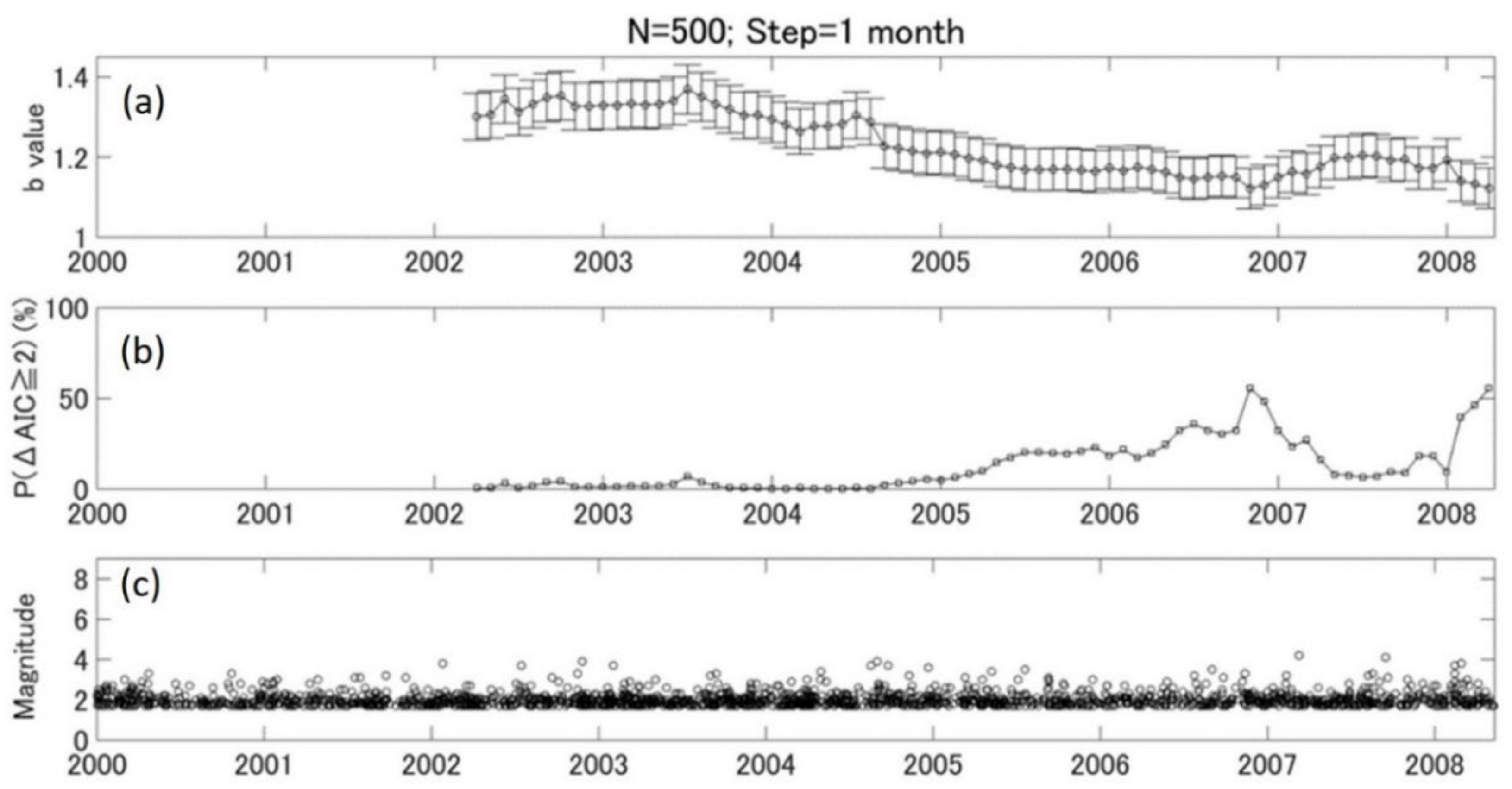
3.2. Estimation of b Values
3.3. Significance Level of b-Value Changes
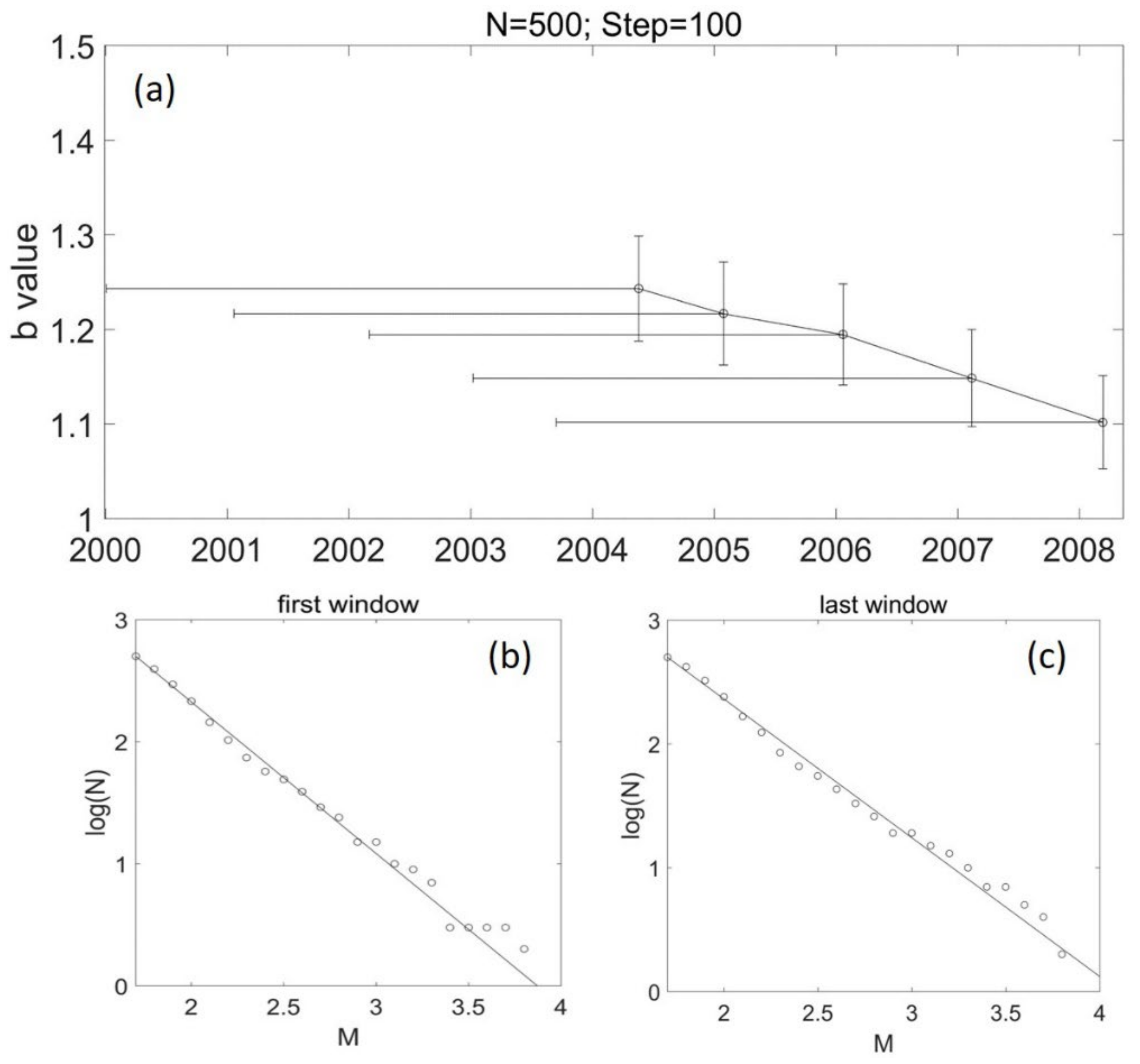
4. Results
5. Discussion
5.1. Mc Estimation
5.2. b-Value Calculation and the Significance of b-Value Change
5.3. b Value and Stress Evolution
5.4. b Value for Earthquake Forecast
6. Conclusions
Author Contributions
Funding
Data Availability Statement
Acknowledgments
Conflicts of Interest
References
- Gutenberg, R.; Richter, C.F. Frequency of earthquakes in California. Bull. Seismol. Soc. Am. 1944, 34, 185–188. [Google Scholar] [CrossRef]
- Schorlemmer, D.; Wiemer, S.; Jackson, D. Earthquake statistics at Parkfield: 1. Stationality of b values. J. Geophys. Res. Solid Earth 2004, 109, 12307. [Google Scholar] [CrossRef]
- Scholz, C.H. On the stress dependence of the earthquake b value. Geophys. Res. Lett. 2015, 42, 1399–1402. [Google Scholar] [CrossRef] [Green Version]
- Mousavi, M.; Ogwari, P.; Horton, S.; Langston, C. Spatio-temporal evolution of frequency-magnitude distribution and seismogenic index during initiation of induced seismicity at Guy-Greenbrier, Arkansas. Phys. Earth Planet. Inter. 2017, 267, 53–66. [Google Scholar] [CrossRef]
- Tan, Y.J.; Waldhauser, F.; Tolstoy, M.; Wilcock, W. Axial Seamount: Periodic tidal loading reveals stress dependence of the earthquake size distribution (b value). Earth Planet. Sci. Lett. 2019, 512, 39–45. [Google Scholar] [CrossRef] [Green Version]
- Xie, W.; Hattori, K.; Han, P.; Shi, H. Temporal variation and statistical assessment of b value off the Pacific coast of Tokachi, Hokkaido, Japan. Entropy 2019, 21, 249. [Google Scholar] [CrossRef] [Green Version]
- Nuannin, P.; Kulhanek, O.; Persson, L. Spatial and temporal b value anomalies preceding the devastating off coast of NW Sumatra earthquake of December 26, 2004. Geophys. Res. Lett. 2005, 32, 32. [Google Scholar] [CrossRef]
- Nanjo, K.Z.; Hirata, N.; Obara, K.; Kasahara, K. Decade-scale decrease in b value prior to the M9-class 2011 Tohoku and 2004 Sumatra quakes. Geophys. Res. Lett. 2012, 39, 20304. [Google Scholar] [CrossRef]
- Nanjo, K.; Yoshida, A. Anomalous decrease in relatively large shocks and increase in the p and b values preceding the April 16, 2016, M7.3 earthquake in Kumamoto, Japan. Earth Planets Space 2017, 69, 13. [Google Scholar] [CrossRef] [Green Version]
- Nanjo, K. Were changes in stress state responsible for the 2019 Ridgecrest, California, earthquakes? Nat. Commun. 2020, 11, 3082. [Google Scholar] [CrossRef]
- Wang, R.; Chang, Y.; Miao, M.; Zeng, Z.; Chen, H.; Shi, H.; Li, D.; Liu, L.; Su, Y.; Han, P. Assessing Earthquake Forecast Performance Based on b Value in Yunnan Province, China. Entropy 2021, 23, 730. [Google Scholar] [CrossRef] [PubMed]
- Varotsos, P.A.; Sarlis, N.V.; Skordas, E.S. Order parameter fluctuations in natural time and b-value variation before large earthquakes. Nat. Hazards Earth Syst. Sci. 2012, 12, 3473–3481. [Google Scholar] [CrossRef] [Green Version]
- Varotsos, P.A.; Sarlis, N.V.; Skordas, E.S. Study of the temporal correlations in the magnitude time series before major earthquakes in Japan. J. Geophys. Res. Space Phys. 2014, 119, 9192–9206. [Google Scholar] [CrossRef]
- Sarlis, N.V.; Skordas, E.S.; Varotsos, P.A. Order parameter fluctuations of seismicity in natural time before and after mainshocks. Europhys. Lett. 2010, 91, 59001. [Google Scholar] [CrossRef] [Green Version]
- Sarlis, N.V.; Skordas, E.S.; Varotsos, P.A.; Nagao, T.; Kamogawa, M.; Uyeda, S. Spatiotemporal variations of seismicity before major earthquakes in the Japanese area and their relation with the epicentral locations. Proc. Natl. Acad. Sci. USA 2015, 112, 986–989. [Google Scholar] [CrossRef] [PubMed] [Green Version]
- Gulia, L.; Wiemer, S. Real-time discrimination of earthquake foreshocks and aftershocks. Nature 2019, 574, 193–199. [Google Scholar] [CrossRef] [PubMed]
- Scholz, C. Microfractures, aftershocks, and seismicity. Bull. Seismol. Soc. Am. 1968, 58, 1117–1130. [Google Scholar]
- Lei, X.L. How do asperities fracture? An experimental study of unbroken asperities. Earth Planet. Sci. Lett. 2003, 213, 347–359. [Google Scholar] [CrossRef]
- Woessner, J.; Wiemer, S. Assessing the Quality of Earthquake Catalogues: Estimating the Magnitude of Completeness and Its Uncertainty. Bull. Seismol. Soc. Am. 2005, 95, 684–698. [Google Scholar] [CrossRef]
- Hattori, K.; Han, P.; Yoshino, C.; Febriani, F.; Yamaguchi, H.; Chen, C.H. Investigation of ULF Seismo-Magnetic Phenomena in Kanto, Japan During 2000–2010: Case Studies and Statistical Studies. Surv. Geophys. 2013, 34, 293–316. [Google Scholar] [CrossRef]
- Han, P.; Hattori, K.; Hirokawa, M.; Zhuang, J.; Chen, C.H.; Febriani, F.; Yamaguchi, H.; Yoshino, C.; Liu, J.Y.; Yoshida, S. Statistical analysis of ULF seismo-magnetic phenomena at Kakioka, Japan, during 2001–2010. J. Geophys. Res. Space Phys. 2014, 119, 4998–5011. [Google Scholar] [CrossRef]
- Han, P.; Hattori, K.; Zhuang, J.; Chen, C.H.; Liu, J.Y.; Yoshida, S. Evaluation of ULF seismo-magnetic phenomena in Kakioka, Japan by using Molchan’s error diagram. Geophys. J. Int. 2017, 208, 482–490. [Google Scholar] [CrossRef]
- Liu, C.Y.; Liu, J.Y.; Chen, Y.I.; Qin, F.; Chen, W.S.; Xia, Y.Q.; Bai, Z.Q. Statistical analyses on the ionospheric total electron content related to M ≥ 6.0 earthquakes in China during 1998–2015. Terr. Atmos. Ocean. Sci. 2018, 29, 485–498. [Google Scholar] [CrossRef] [Green Version]
- Hattori, K.; Han, P. Statistical Analysis and Assessment of Ultralow Frequency Magnetic Signals in Japan As Potential Earthquake Precursors. In Pre-Earthquake Processes: A Multidisciplinary Approach to Earthquake Prediction Studies; Ouzounov, D., Pulinets, S., Hattori, K., Taylor, P., Eds.; Wiley: Hoboken, NJ, USA, 2018; pp. 229–240. [Google Scholar] [CrossRef]
- Ouzounov, D.; Pulinets, S.; Liu, J.Y.; Hattori, K.; Han, P. Multiparameter Assessment of Pre-Earthquake Atmospheric Signals. Pre-Earthquake Processes: A Multidisciplinary Approach to Earthquake Prediction Studies; Ouzounov, D., Pulinets, S., Hattori, K., Taylor, P., Eds.; Wiley: Hoboken, NJ, USA, 2018; pp. 339–359. [Google Scholar] [CrossRef]
- Han, P.; Zhuang, J.; Hattori, K.; Chen, C.H.; Febriani, F.; Chen, H.; Yoshino, C.; Yoshida, S. Assessing the potential earthquake precursory information in ULF magnetic data recorded in Kanto, Japan during 2000–2010: Distance and magnitude dependences. Entropy 2020, 22, 859. [Google Scholar] [CrossRef]
- Genzano, N.; Filizzola, C.; Hattori, K.; Pergola, N.; Tramutoli, V. Statistical correlation analysis between thermal infrared anomalies 1 observed from MTSATs and large earthquakes occurred in Japan (2005–2015). J. Geophys. Res. Solid Earth 2021, 126, e2020JB020108. [Google Scholar] [CrossRef]
- Yu, Z.; Hattori, K.; Zhu, K.; Fan, M.; He, X. Evaluation of pre-earthquake anomalies of borehole strain network by using Receiver Operating Characteristic Curve. Remote Sens. 2021, 13, 515. [Google Scholar] [CrossRef]
- Utsu, T. On seismicity, in report of the Joint Research Institute for Statistical Mathematics. Inst. Stat. Math. Tokyo 1992, 34, 139–157. (In Japanese) [Google Scholar]
- Schorlemmer, D.; Wiemer, S.; Wyss, M.; Jackson, D. Earthquake statistics at Parkfield: 2. Probabilistic forecasting and testing. J. Geophys. Res. Solid Earth 2004, 109, 12308. [Google Scholar] [CrossRef] [Green Version]
- He, P.C.; Shen, Z.K. Rupture triggering process of Wenchuan earthquake seismogenic faults. Chin. J. Geophys.Chin. Ed. 2014, 57, 3308–3317. (In Chinsese) [Google Scholar]
- Wiemer, S.; Wyss, M. Minimum magnitude of complete reporting in earthquake catalogs: Examples from Alaska, the WesternUnited States, and Japan. Bull. Seismol. Soc. Am. 2000, 90, 859–869. [Google Scholar] [CrossRef]
- Aki, K. Maximum likelihood estimate of b in the formula log N= a-bM and its confidence limits. Bull. Earthq. Res. Inst. 1965, 43, 237–239. [Google Scholar]
- Utsu, T. A method for determining the value of b in a formula log n=a-bM showing themagnitude-frequency relation for earthquakes. Geophys. Bull. Hokkaido Univ. 1965, 13, 99–103. (In Japanese) [Google Scholar]
- Nava, F.A.; Márquez-Ramírez, V.H.; Zúñiga, F.R.; Ávila-Barrientos, L.; Quinteros, C.B. Gutenberg-Richter b-value maximum likelihood estimation and sample size. J. Seismol. 2017, 21, 127–135. [Google Scholar] [CrossRef]
- Liu, R.F.; Wu, Z.L.; Yin, C.M.; Chen, Y.T.; Zhuang, C.T. Development of China Digital Seismological Observational Systems. Acta Seismol. Sin. 2003, 16, 568–573. [Google Scholar]
- Shi, Y.; Bolt, B.A. The standard error of the magnitude-frequency b value. Bull. Seismol. Soc. Am. 1982, 72, 1677–1687. [Google Scholar] [CrossRef]
- Stumpf, M.P.; Porter, M.A. Critical Truths About Power Laws. Science 2012, 335, 665–666. [Google Scholar] [CrossRef] [PubMed]


Publisher’s Note: MDPI stays neutral with regard to jurisdictional claims in published maps and institutional affiliations. |
© 2022 by the authors. Licensee MDPI, Basel, Switzerland. This article is an open access article distributed under the terms and conditions of the Creative Commons Attribution (CC BY) license (https://creativecommons.org/licenses/by/4.0/).
Share and Cite
Xie, W.; Hattori, K.; Han, P.; Shi, H. Temporal Variation of b Value with Statistical Test in Wenchuan Area, China Prior to the 2008 Wenchuan Earthquake. Entropy 2022, 24, 494. https://doi.org/10.3390/e24040494
Xie W, Hattori K, Han P, Shi H. Temporal Variation of b Value with Statistical Test in Wenchuan Area, China Prior to the 2008 Wenchuan Earthquake. Entropy. 2022; 24(4):494. https://doi.org/10.3390/e24040494
Chicago/Turabian StyleXie, Weiyun, Katsumi Hattori, Peng Han, and Haixia Shi. 2022. "Temporal Variation of b Value with Statistical Test in Wenchuan Area, China Prior to the 2008 Wenchuan Earthquake" Entropy 24, no. 4: 494. https://doi.org/10.3390/e24040494