Abstract
Texture analysis is a subject of intensive focus in research due to its significant role in the field of image processing. However, few studies focus on colored texture analysis and even fewer use information theory concepts. Entropy measures have been proven competent for gray scale images. However, to the best of our knowledge, there are no well-established entropy methods that deal with colored images yet. Therefore, we propose the recent colored bidimensional fuzzy entropy measure, , and introduce its new multi-channel approaches, and , for the analysis of colored images. We investigate their sensitivity to parameters and ability to identify images with different irregularity degrees, and therefore different textures. Moreover, we study their behavior with colored Brodatz images in different color spaces. After verifying the results with test images, we employ the three methods for analyzing dermoscopic images of malignant melanoma and benign melanocytic nevi. , , and illustrate a good differentiation ability between the two—similar in appearance—pigmented skin lesions. The results outperform those of a well-known texture analysis measure. Our work provides the first entropy measure studying colored images using both single and multi-channel approaches.
1. Introduction
Texture features are of the utmost importance in segmentation, classification, and synthesis of images, to cite only few image processing steps. However, no precise definition of texture has been adopted yet. Texture is often referred to as the visual patterns appearing in the image. Several algorithms have been proposed for texture feature extraction in recent years and this research area is still the subject of many investigations [1,2,3,4,5,6,7,8,9,10]. Recently, seven classes were proposed to classify the texture feature extraction methods [1]: statistical approaches (among which we can find the co-occurrence matrices), structural approaches, transform-based approaches (Fourier transform-based approaches, among others), model-based approaches (such as the random field models), graph-based approaches (such as the local graph structures), learning-based approaches, and entropy-based approaches. The latter two classes (learning-based approaches and entropy-based approaches) are the most recent ones. Several studies have shown that the entropy-based measures are promising for texture analysis [11,12,13,14,15,16,17,18]. However, these studies are only at their beginning. Even if they have the great advantage of relying on reliable unidimensional, 1D, entropy-based measures (issued from the information theory field), they have the drawback—for most of them—of being designed for gray scale images only.
Besides texture, color is essential not only for human perception of images but also for digital image processing [19,20,21,22,23,24,25]. Unlike the intensity that is translated as scalar gray values for a gray scale image, color is a vectorial feature that is appointed to each pixel for a colored image [19]. In contrast to gray scale images that could be handled in a straightforward manner, colored images could be analyzed in several possible ways. This depends on many factors, such as the need to analyze texture or color, separately or combined, directly from the image or through a transformation, among other factors [19,24,25,26]. Only a few studies have been performed on colored texture analysis and most of them were achieved by adapting the application of gray scale textures analysis methods [13,18,27,28]. Nevertheless, color and texture are probably the most important components of visual features. Many biomedical images are color-textured: dermoscopy images, histological images, endoscopy data, fundus and retinal images, among others.
According to the World Health Organization, one in every three diagnosed cancer cases is a skin cancer and the incidence rate has been increasing over recent years. A non-invasive imaging modality, dermoscopy or epiluminescence microscopy (ELM), is one of the well-known non-invasive techniques used for skin cancer diagnosis on which most research studies are conducted. However, visual diagnosis alone might be misleading and subjective even when performed by experts. Thus, dermoscopy image analysis (DIA) using computer-aided diagnosis (CAD) systems is essential to help medical doctors. Several studies proposed computer extracted texture features for cutaneous lesions diagnosis, specifically for the most aggressive type, melanoma [29,30,31]. Melanoma is metastatic, thus its early diagnosis and excision would definitely increase the survival rate. Some DIA methods focus only on the dermoscopic image structure/patterns [32,33], others rely on colors [34,35,36], and some consider both [37], for more details please refer to [29,30,31]. Nevertheless, most studies propose learning-based approaches and only few have suggested entropy-based measures until now.
In this paper, we, therefore, propose novel bidimensional entropy-based measures dedicated to color images in their two approaches: single-channel approach, , and multi-channel approaches, and . First, we test the abilities of our proposed measures in colored texture analysis on different kinds of image. After that, we illustrate their application in the biomedical field by processing dermoscopic images of two different kinds of common pigmented lesions: melanoma and benign melanocytic nevi. Furthermore, our results are compared to one of the most well-known texture feature extraction methods (co-occurrence matrices).
2. Colored Bidimensional Fuzzy Entropy
We recently developed bidimensional fuzzy entropy, , and its multi-scale extension [17,18,38]. These entropy measures revealed interesting results for some dermoscopic images but were limited to gray scale images. Based on , we propose herein approaches to deal with colored images: the single-channel bidimensional fuzzy entropy, [28] which considers the characteristics of each channel independently, and the multi-channel bidimensional fuzzy entropy measures, and , which take into consideration the inter-channel characteristics. In this paper, we limit our study to three color channels. However, extension to a higher number of channels would be straightforward. For a colored image U of W width, H height, and K channels ( pixels), the following initial parameters are first set: tolerance level r, fuzzy power n, and window size m (see below). The algorithms to compute , , and are presented below.
2.1. Single-Channel Approach
The colored image U is separated into its corresponding color channels , , and , as U, U, and U, respectively. For each channel composed of elements, X is designated as the m-length square window:
with K = , , or and the indices are defined as such: and . The square window, X, is defined in the same way. In each of U, U, and U, the total number of defined square windows for both m and sizes is .
Based on the original fuzzy entropy definition, [39], a distance function between X and its neighboring windows X is defined as the maximum absolute difference in their corresponding scalar components. We compose as follows:
with a ranging from 1 to and b ranging from 1 to . The similarity degree of X with its neighboring patterns X is defined by a continuous fuzzy function :
Afterwards, the similarity degree of each X is averaged to obtain and then construct:
It is similar for patterns to obtain . Consequently, of each channel is calculated as:
Finally, is defined in each channel as the natural logarithm of the conditional probability that patterns with similar pixels would remain similar for the next pixels in each channel:
This single-channel approach treats each channel independently. It has the advantage of allowing us to selectively study certain channels which is of special importance when it comes to images in different color spaces and natures (intensity, color, and texture). In our study, we used . Thus, the similarity degree is expressed by a Gaussian function . For better illustration, we show in Figure 1 an example for of an RGB color space image for an embedding dimension of m = [2, 2]; i.e., pixels for each channel. The illustration shows RGB channels as an example, but the same could be applied to different color spaces.
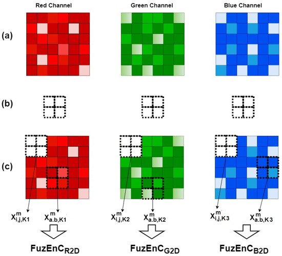
Figure 1.
Illustration for of an RGB color space image. (a) The image U is split into its corresponding channels U, U, and U, respectively, from left to right; (b) the embedding dimension pattern of size having m; (c) X and X for K = K1, K2, and K3 being the R, G, and B color channels, respectively.
2.2. Multi-Channel Approach
For an image U composed of pixels, X is defined as the m-length cube. X represents the group of pixels in the image U of indices from line i to , column j to , and the depth of K-channels (k: depth index) as follows:
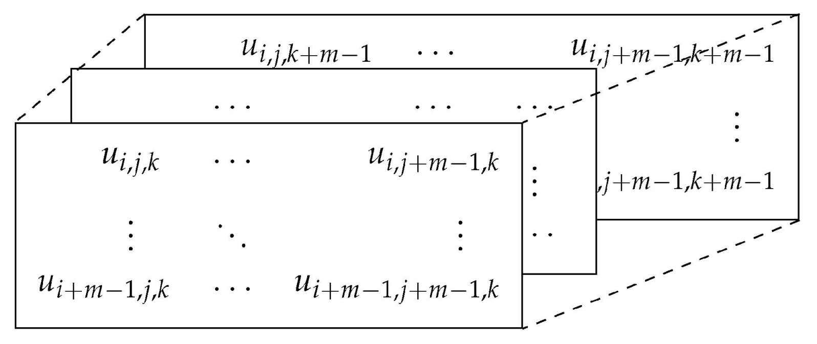
Similarly, X is defined as the -length cube. Let be the total number of cubes that can be generated from U for both m and sizes. For X and its neighboring cubes X, the distance function between them is defined as the maximum absolute difference of their corresponding scalar components, knowing that a, b, and c range from 1 to , , and , respectively. Having , the distance function is depicted as follows:
The similarity degree of X with its neighboring cubes X is defined by a fuzzy function :
Afterwards, the similarity degree of each cube is averaged to obtain , then construct:
This is similar for cubes to obtain . Finally, multi-channel bidimensional fuzzy entropy of the colored image is defined as the natural logarithm of the conditional probability that cubes similar in their pixels would remain similar for the next pixels:
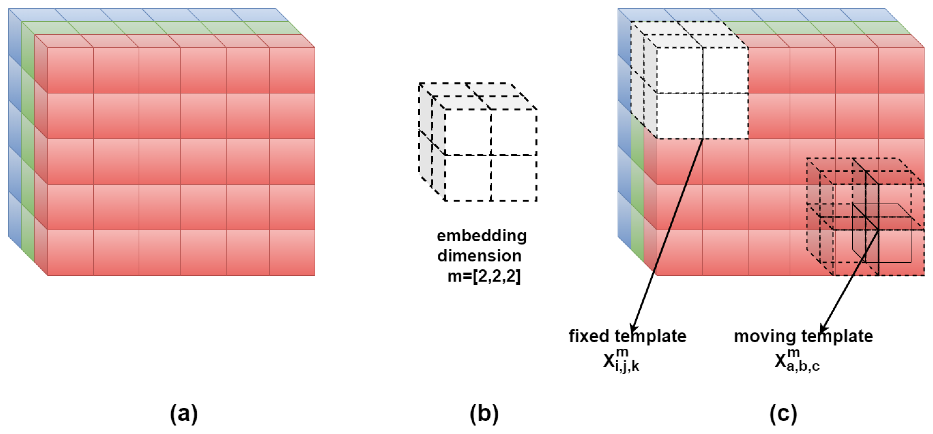
The multi-channel approach has the advantage of extracting inter-channel features. However, we limit our study herein to 3-channel colored images. Thus, the embedding dimension m values could be 1 or 2 to avoid exceeding the maximum possible pixels cubes for the calculations. This means that for K channels the m-value can only be defined between 1 and K-1. Herein, n is taken to be 2 and r within the range suggested in previous studies. For better illustration, we show in Figure 2 an example for of an RGB color space image for an embedding dimension of m = [2, 2, 2].

Figure 2.
Illustration for of an RGB color space image having m = [ 2,2,2]. (a) A portion of the colored image with its R, G, and B channels; (b) the scanning pattern or embedding dimension with m that is a cube; (c) X and X, the fixed and moving templates defined above.
2.3. Modified Multi-Channel Approach
Since the embedding dimension size is limited to m = 1 and m = 2 for this trichromatic study (K = 3), we introduce herein a modified colored multi-channel approach that can take up to any m value. This method is similar to except for the fact that the embedding dimension is a cuboid of voxels for . Therefore, the third dimension of the template is not limited by the number of color channels in the study.
For image U with K = 3 color channels, composed of voxels, X is defined as the cuboid. X represents the group of voxels in the image U of indices from line i to , column j to , and the depth of K-channels (k: depth index). Similarly, X is defined as the cuboid. Let be the total number of cuboids that can be generated from U for both m and sizes. Sizes m and stand for [m, m, 3] and [, , 3] that are made up of and voxels, respectively.
For X and its neighboring cuboids X, the distance function between them is defined as the maximum absolute difference of their corresponding scalar components, knowing that a and b range from 1 to and , respectively, whereas c is 1. Having , the distance function is depicted as follows:
The similarity degree of X with its neighboring cuboids X is defined by a fuzzy function :
Afterwards, the similarity degree of each cuboid is averaged to obtain , then construct:
This is similar for cuboids to obtain . Finally, multi-channel bidimensional fuzzy entropy of the colored image is defined as the natural logarithm of the conditional probability that cuboids similar in their voxels would remain similar in their voxels:
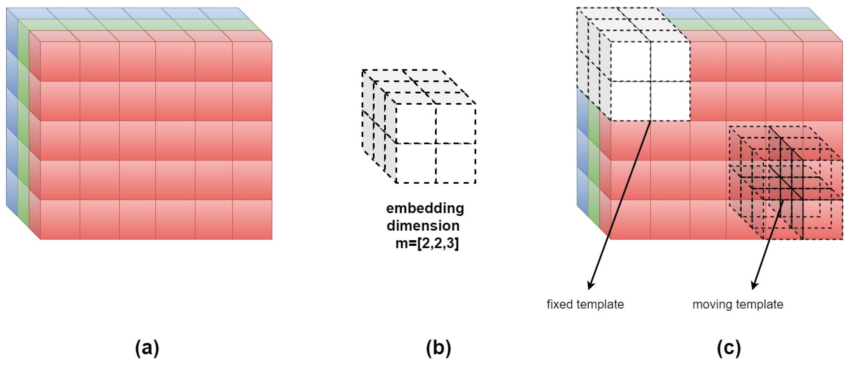
has the advantage of extracting inter-channel features and always considering all the color channels of texture images. However, as mentioned previously, we consider our study herein for 3-channel colored images which could be further adapted to a higher number as well. Herein, n is taken to be 2 and r within the range suggested in previous studies. For better illustration, we show in Figure 3 an example for of an RGB color space image for an embedding dimension of m = [2, 2, 3]; i.e., moving m-sized cuboid is .

Figure 3.
Illustration for of RGB color space image having m. (a) A portion of the colored image with its R, G, and B channels; (b) the scanning pattern or embedding dimension with m that is a cuboid; (c) the fixed and moving templates defined above.
2.4. Comparing Algorithms
The proposed entropy measures are based on the fuzzy entropy definition [17,39,40] that calculates the similarity degree between the corresponding patterns using a continuous fuzzy function. The latter ensures calculating a participation degree for all the compared patterns and quantifies the irregularity of the analyzed data. This information theory concept has been proven to be reliable for 1D, 2D, and 3D data [17,18,38,39,40]. However, only gray scale data have been investigated to date. Therefore, the idea to analyze colored texture images using the fuzzy entropy concept from a single channel and a multi-channel perspective is interesting.
The major differences between the three proposed algorithms are in the way the similarity degrees are calculated. For the single-channel approach, , the image is analyzed channel by channel and the result is three entropy values that represent the three channels, respectively, please refer to Figure 1. This is a particular advantage when it comes to analyzing and comparing specific channels in different color spaces. On the other hand, the multi-channel approaches, and , deal with all the channels at the same time; i.e., the inter-channel information is taken into account (unlike handling each color channel separately). transforms the 2D similarity degree scanning window into a 3D cubic pattern that studies similarity among the and the patterns within a colored image. showed good results but for the application in trichromatic color spaces the embedding dimension size was limited to m = 1 or 2, please see Figure 2. Therefore, in order to investigate similarity degrees with larger embedding dimension sizes, we present the modified multi-channel approach , please refer back to Figure 3. , , and provide colored texture analysis from single-channel and multi-channel perspectives. The choice of the algorithm depends on the intended application. Moreover, the analysis could be extended to multi-spectral images and even other color spaces than the ones discussed in this paper.
3. Validation Tests and Medical Database
In order to validate the proposed colored bidimensional entropy measures, we studied their sensitivity to different parameter values. The algorithms were also tested using images with different degrees of randomness and the colored Brodatz dataset [41]. The images were normalized by subtracting their mean and dividing by their standard deviation and all the tests were performed using Matlab. In the following, we describe the elements used for the validation tests and the medical dataset.
3.1. MIX(p) Processes
MIX(p) [12] is a family of images of stochastic processes that are moderated by the probability of irregularity, p, varying from 0 (totally regular periodic image) to 1 (totally irregular image). We used MIX(p) for the single-channel approach, and MIX(p), a volumetric extension for MIX(p) proposed by [40], for our multi-channel approach.
3.2. Colored Brodatz Images
For texture validation tests, we used the colored Brodatz texture (CBT) [41,42] images, see Figure 4. CBT presents colored textures with different degrees of visible irregularity. We can notice that, for example, the CBT images (a), (b) and (e) show more regular and periodic repetitive patterns than (c), (f) and (i).
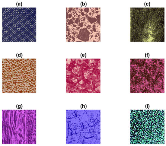
Figure 4.
Colored Brodatz texture (CBT) images of different colored irregularity degrees [41,42]. (a–i) CBT images that are used for the validation test (Section 4.3) to compare the entropy values of each colored texture to its corresponding sub-images in three color spaces (RGB, HSV, and YUV); (f) is used again for studying the sensitivity of the proposed measures to different initial parameters (Section 4.1).
3.3. Color Spaces
Besides using the most common trichromatic color space, red, green, blue (RGB), we extend our study by transforming the images to use two other color spaces: hue, saturation, value (HSV; hue and saturation: chrominance, value: intensity) and YUV (Y: luminance, U and V: chrominance) to investigate the effect of color space transformations on , , and outcomes. In RGB color space, the intensity and color are combined to give us the final display, whereas for HSV and YUV color spaces, intensity and color are separated.
3.4. Co-Occurrence Matrices
For the application on medical images, we study the effect of different color spaces and compare our results to those obtained with gray level co-occurrence matrices [43], which probably remains the most used texture analysis technique. We employed the co-occurrence matrices of each channel (integrative way) for comparing the results to our single-channel approach, and its extended 3D co-occurrence matrices [44] for comparing the results to our multi-channel approach. We thus adopted the following procedure:
- The 2D co-occurrence matrices were created considering 4 orientations (0, 45, 90, and 135), 4 inter-pixel distances (1, 2, 4, and 8), and 8 gray levels ( = 8) to be compared with .
- The 3D co-occurrence matrices were created considering 13 orientations [44], 4 inter-pixel distances (1, 2, 4, and 8), and 8 gray levels to be compared with and .
Then, we calculated the Haralick features for each co-occurrence matrix (for each orientation and distance). Finally, the average of features for all matrices was calculated to be compared with , , and values. Among the 14 features originally proposed [43], only six are commonly employed by researchers due to their correlation with the other eight, see Table 1.

Table 1.
Definition of the computed Haralick features [43].
3.5. Medical Images
For our medical application we used the HAM10000, “Human Against Machine with 10,000 training images” [45,46]. The dataset is composed of dermoscopic images for pigmented lesions, see an example in Figure 5a. The dataset contains dermoscopic images of melanocytic nevi, melanoma, dermatofibroma, actinic keratoses, basal cell carcinoma, and benign keratosis [45].
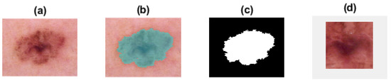
Figure 5.
Dermoscopic images segmentation for choosing the region of interest (ROI). (a) an example of the dermoscopic image for a pigmented skin lesion; (b,c) the contouring and segmentation of the lesion; (d) the ROI as the central pixels.
As suggested by medical doctors, the most significant comparison is that between melanoma and melanocytic nevi. The target of the medical application in our study is to try to differentiate the deadliest type of skin cancer, melanoma, from the benign melanocytic nevi. These two widespread types of pigmented skin lesions are often mistaken in diagnosis and detection, especially in their early stages. Moreover, early diagnosis and excision could vastly increase the patients’ survival rate [29,30,31]. Thus, we selected from the proposed dataset forty melanoma images and forty melanocytic nevi images to be processed and compared.
4. Results and Discussion
In this section, we present the results of the validation tests. We start by testing the algorithms’ sensitivity to initial parameter choice, then we explore the algorithms’ ability to identify increasing irregularity degrees in colored textures. After that, we analyze colored Brodatz texture images in 3 different color spaces (RGB, YUV, and HSV). Finally, we show the results using , , and for melanoma and melanocytic nevi dermoscopic images and compare them to those obtained using single-channel and multi-channel co-occurrence matrices.
4.1. Sensitivity to Initial Parameters
To study the sensitivity of our proposed measures, with different embedding dimensions m and tolerance levels r, we evaluated 100 × 100 pixels of a colored Brodatz image (Figure 4f) using different parameter choices.
- For , the embedding dimension m was taken as 1, 2, 3, 4, and 5, and the tolerance level r from 0.06 up to 0.48 (step 0.06). The results are displayed in Figure 6.
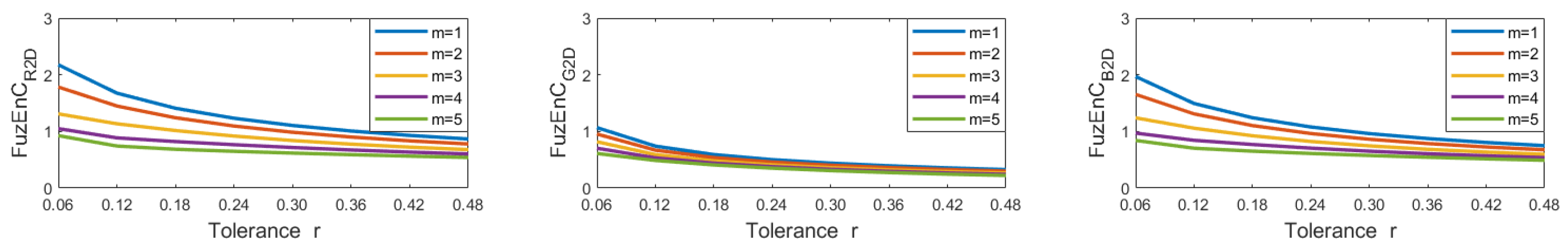
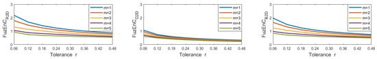 Figure 6. results for the red, green, and blue channels (left to right) of the colored Brodatz image, Figure 4f, with varying r and m.
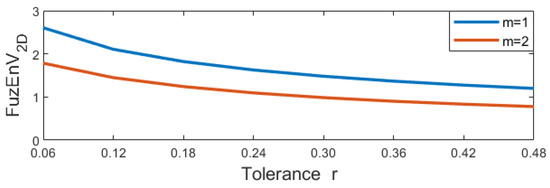
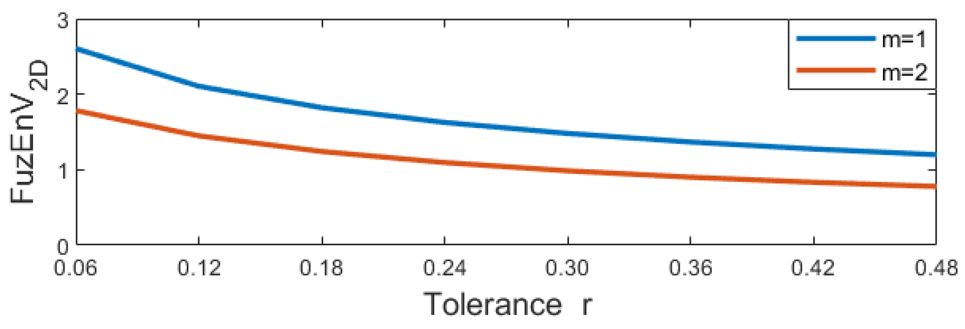
 - For , the embedding dimension m was taken as 1 and 2, since the maximum possible cube volume for -length cubes is pixels (given the 3 color channels). The results are displayed in Figure 7.
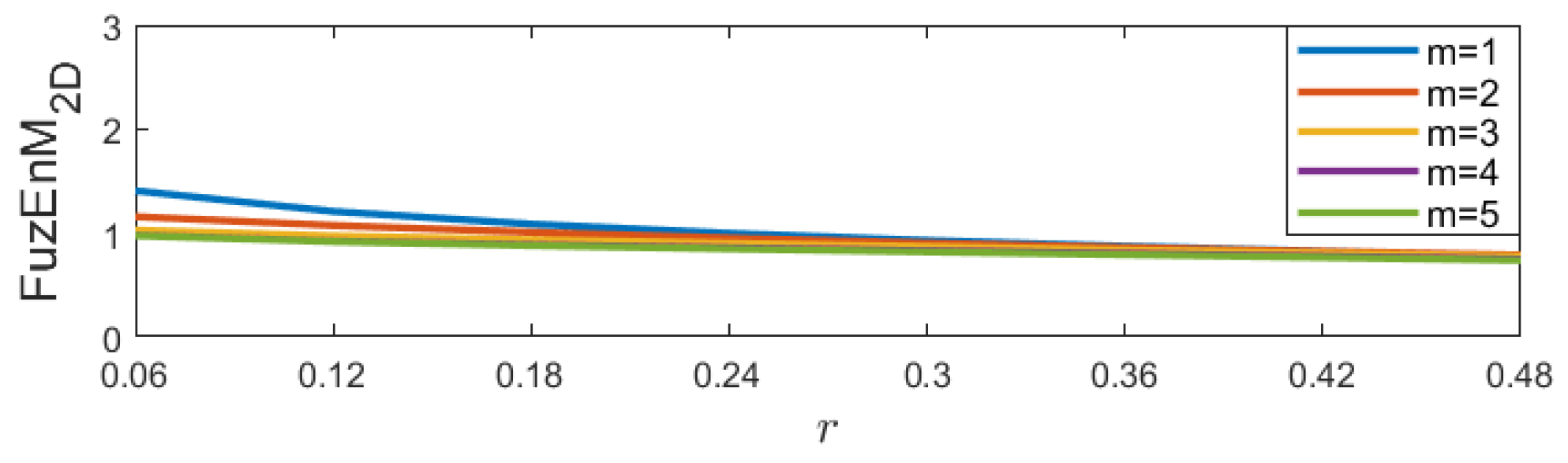
- For , the embedding dimension m was taken as 1, 2, 3, 4, and 5, and the tolerance level r from 0.06 up to 0.48 (step 0.06). The results are displayed in Figure 8.
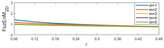
We observe that , , and remain defined for different chosen initial parameters. Additionally, the algorithms show low variability upon changes in r and m. This illustrates their low sensitivity to r and m, allowing a certain degree of freedom in our choice of initial parameters without restrictions.
4.2. Detecting Colored Image Irregularity
We generated pixel MIX(p) in three channels and pixel MIX(p) images and analyzed them by single-channel () and multi-channel approaches ( and ), respectively.
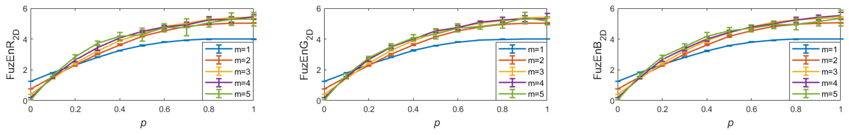
- : we set , , and to 1 with a step of , and repeated the calculation for 10 images each. The results are depicted in Figure 9.
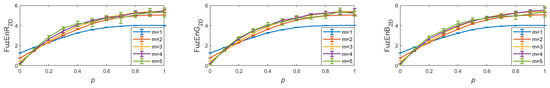 Figure 9. mean and standard deviation for MIX(p) images with 10 repetitions.
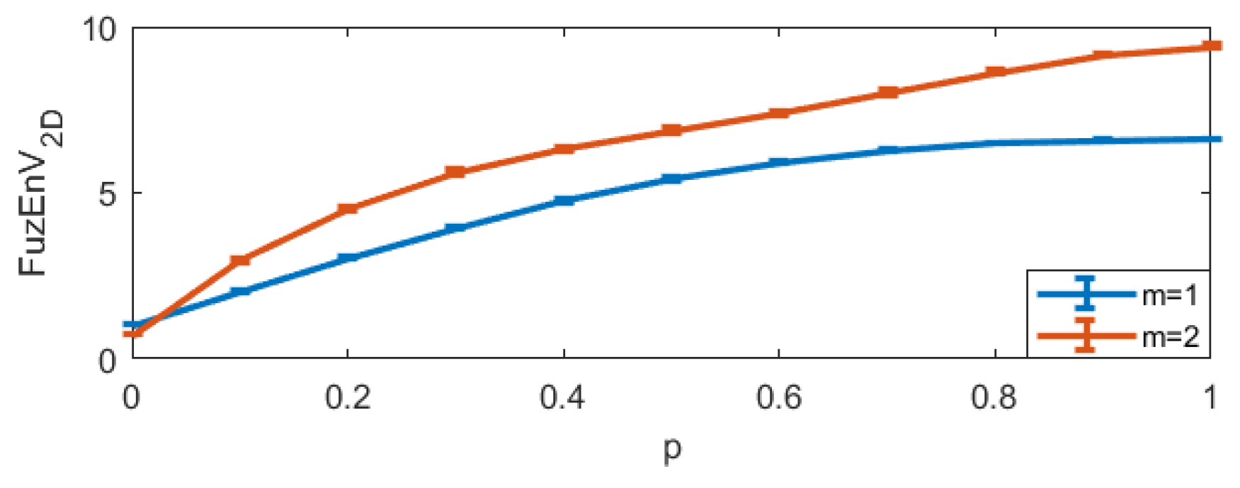
 - : we set , and (as the maximum possible cube volume for could only be pixels), to 1 with a step of , and repeated the calculation for 10 images each. The results are depicted in Figure 10.
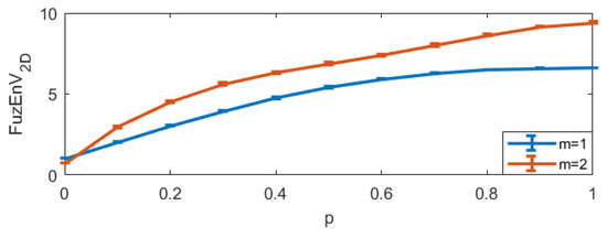 Figure 10. mean and standard deviation for MIX(p) images with 10 repetitions.
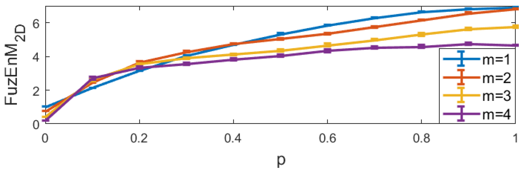
 - : we set , m, and, and to 1 with a step of , and repeated the calculation for 10 images each. The results are depicted in Figure 11.
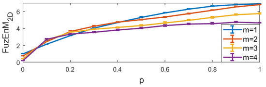 Figure 11. mean and standard deviation for MIX(p) images.
The results show that both the single- and multi-channel approaches lead to increasing entropy values with increasing irregularity degree, p. This illustrates their ability to properly quantify increasing irregularity degrees and their consistency upon repetition.
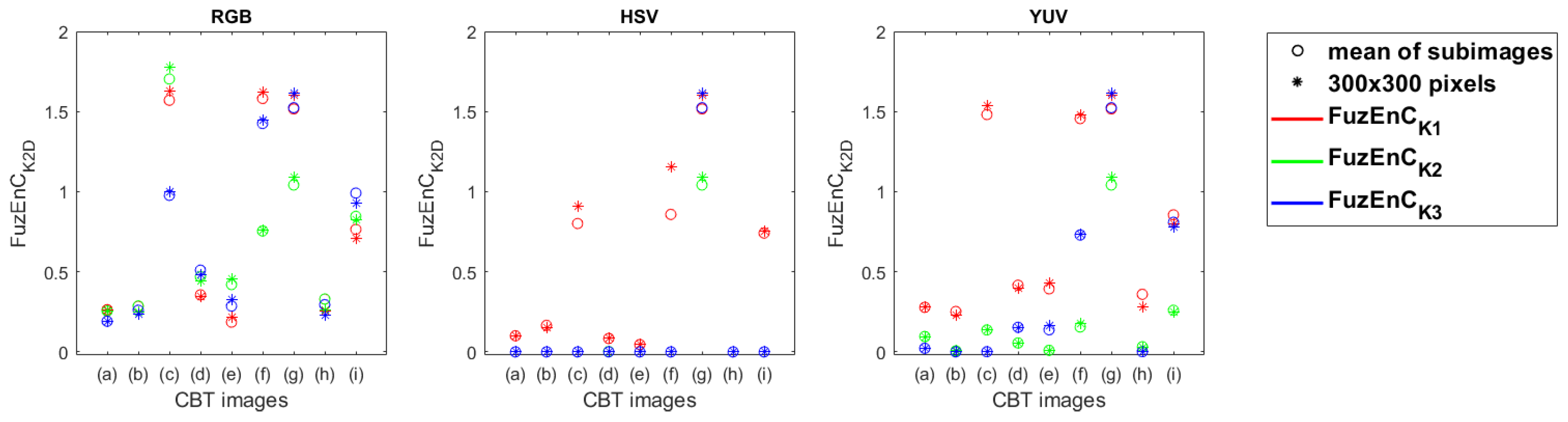
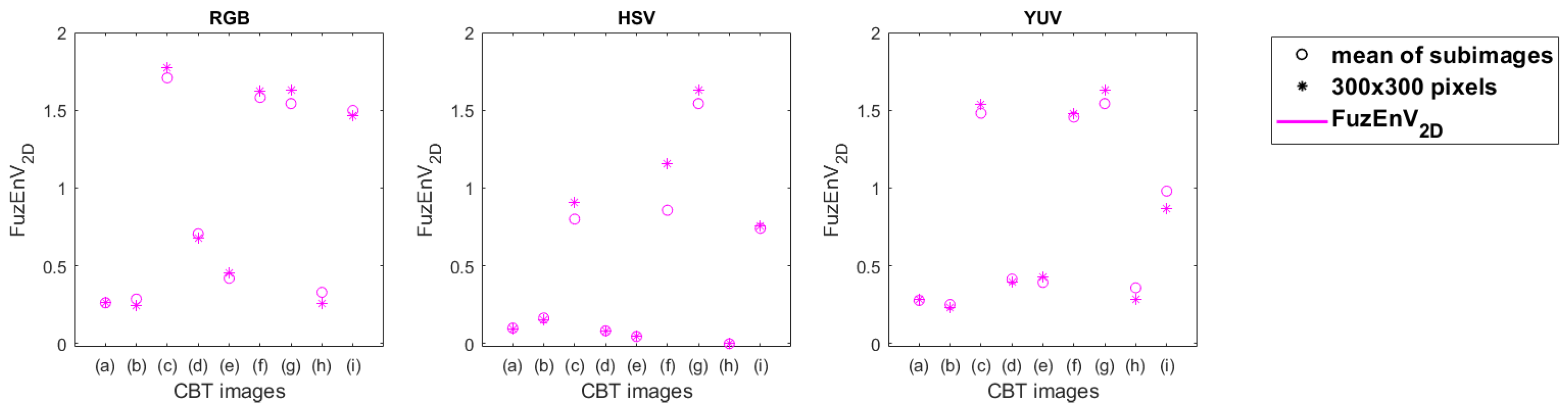
4.3. Studying Texture Images
Nine CBT [41,42] images of 640 × 640 pixels, see Figure 4, were split into 144 sub-images of size 50 × 50 pixels. , , and were calculated for these sub-images and for a 300 × 300 pixel corner region from each corresponding original CBT image. The parameters r and m were set to 0.15 and 2, respectively. The results with and are depicted in Figure 12 and Figure 13. Similar results to those of are found with . We observe that, especially for the RGB color space, most of the , , and averages of the sub-images overlap with or are very similar to the value of their corresponding image’s 300 × 300 pixel region. Moreover, we notice their differentiation ability between different CBT images. In the HSV and YUV color spaces, the multi-channel approaches outperform (Figure 12) in differentiating the CBT images. We can also observe that for the RGB color space, the CBT images that are perceived visually to be of higher color and pattern irregularity, Figure 4c,f,g, obtained higher entropy values than the others, whereas those that appear to be of periodic well-defined repetitive patterns, Figure 4a,b,e, resulted in lower entropy values for the three measures , , and . This is in accordance with the literature of entropy measures and information theory concept applied to gray level texture images [12,14,15,16,17,18,38].
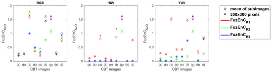
Figure 12.
results for the 144 sub-images and 300 × 300 pixels of the CBT in the three color spaces: RGB, HSV, and YUV, with , , and being the first, second, and third channel, respectively. The mean of the 144 sub-images is displayed as a “∘” sign and the value for the 300 × 300 pixels is displayed as “*”.
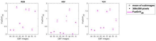
Figure 13.
results for the 144 sub-images and 300 × 300 pixels of the CBT in the three color spaces: RGB, HSV, and YUV. The mean of the 144 sub-images is displayed as a “∘” sign and the value for the 300 × 300 pixels is displayed as “*”.
4.4. Medical Image Analysis
We calculated , , and for 40 melanoma images and 40 melanocytic nevi images from the HAM10000 dataset [45] in the color spaces RGB, HSV, and YUV. In order to determine the region of interest (ROI) of melanoma and melanocytic nevi images, the lesions were segmented as shown in Figure 5. Then, the central region of pixels was selected, see Figure 5d. By adopting this procedure, we ensured that the same number of pixels were processed (equally sized images) and that no region outside the lesion was included. The parameters r and m were set to 0.15 and 2, respectively. The images were normalized by subtracting their mean and dividing by their standard deviation.
To validate the statistical significance of , , and in differentiating melanoma from melanocytic nevi images, we used the Mann–Whitney U test. The resulting p-values are presented in Table 2. shows statistical significance (for p < 0.05) in differentiating melanoma and melanocytic nevi for all the channels except V (of HSV color space). In addition, using and , melanoma and melanocytic nevi images are identified as statistically different for the three color spaces. Moreover, we calculated the Cohen’s d [47,48] to further validate our obtained statistical results, see Table 3. Most d values reflect “large”, “very Large”, and “huge” effect sizes, which validates the differentiation ability of our proposed measures.
Table 2.
Mann–Whitney U test p-values for , , and of 40 melanoma and 40 melanocytic nevi dermoscopic images in the 3 color spaces: RGB, HSV, and YUV, from top to bottom row, respectively.
Table 3.
Cohen’s d-values for , , and of 40 melanoma and 40 melanocytic nevi dermoscopic images in the 3 color spaces: RGB, HSV, and YUV.
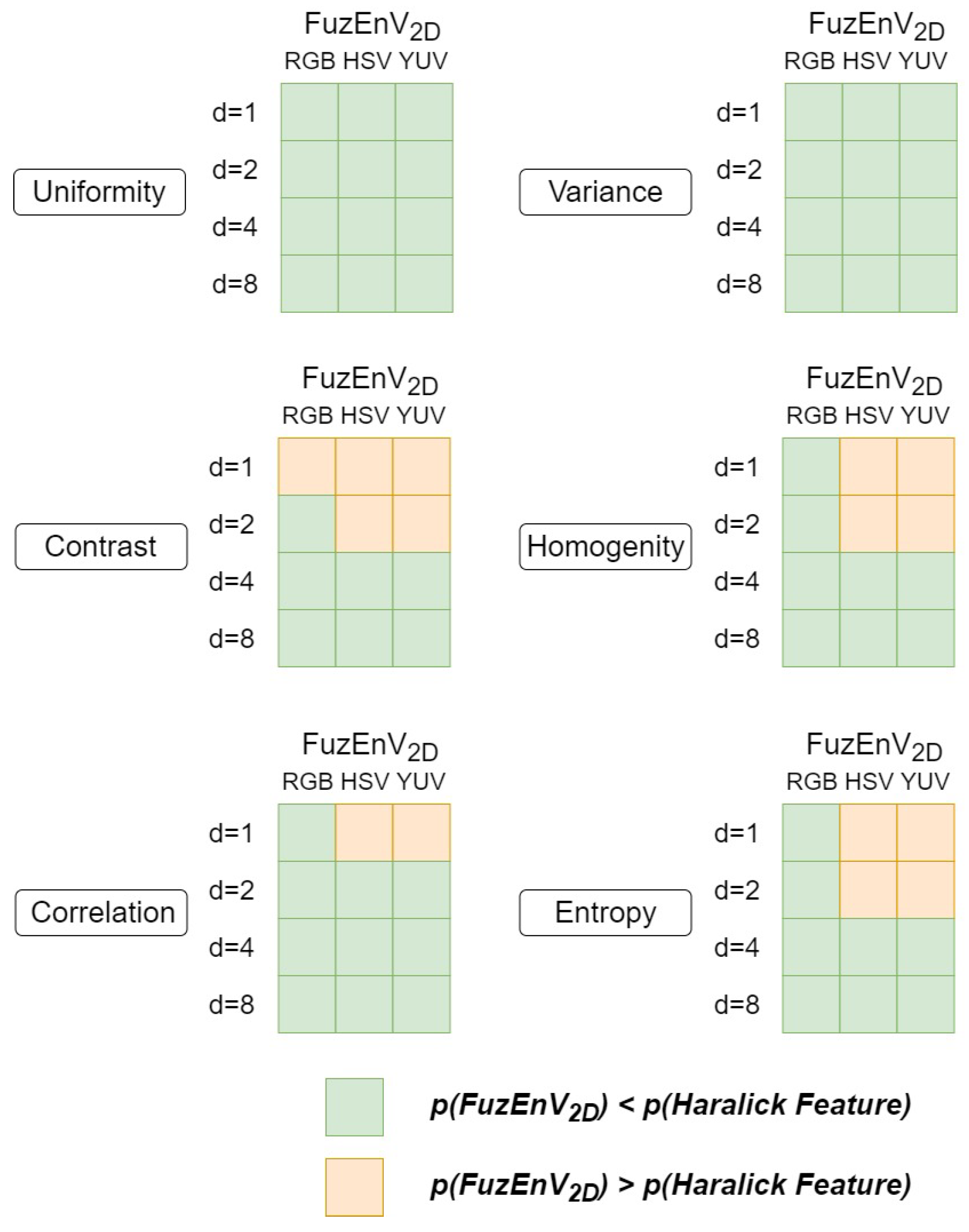
Additionally, we compared results with Haralick features from 2D co-occurrence matrices. The results show that results in lower p-values than Haralick features for the G, H, Y, and U channels and none of the methods result in statistical significance for the S channel. Additionally, we compared and results with Haralick features from 3D co-occurrence matrices. The summaries of results for and are shown in Figure 14 and Figure 15, respectively. and surpassed Haralick features as p-values obtained for the results of both entropy measures are mostly lower than those of Haralick features. Moreover, using Haralick features, some results do not show statistical significance (p > 0.05), whereas all the three proposed colored entropy measures illustrate evident statistical significance in differentiating melanoma from melanocytic nevi, except in results for S and V color channels.
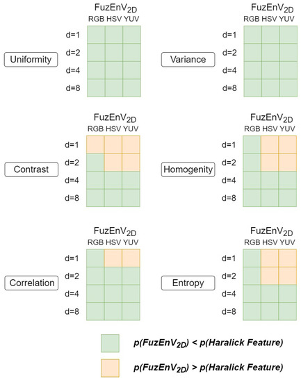
Figure 14.
and Haralick feature p-values of 40 melanoma and 40 melanocytic nevi dermoscopic images in the 3 color spaces: RGB, HSV, and YUV. d represents the inter-pixel distances for the co-occurrence matrices.
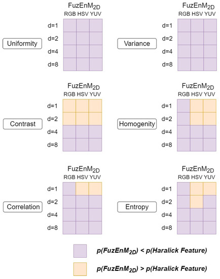
Figure 15.
and Haralick feature p-values of 40 melanoma and 40 melanocytic nevi dermoscopic images in the 3 color spaces: RGB, HSV, and YUV. d represents the inter-pixel distances for the co-occurrence matrices.
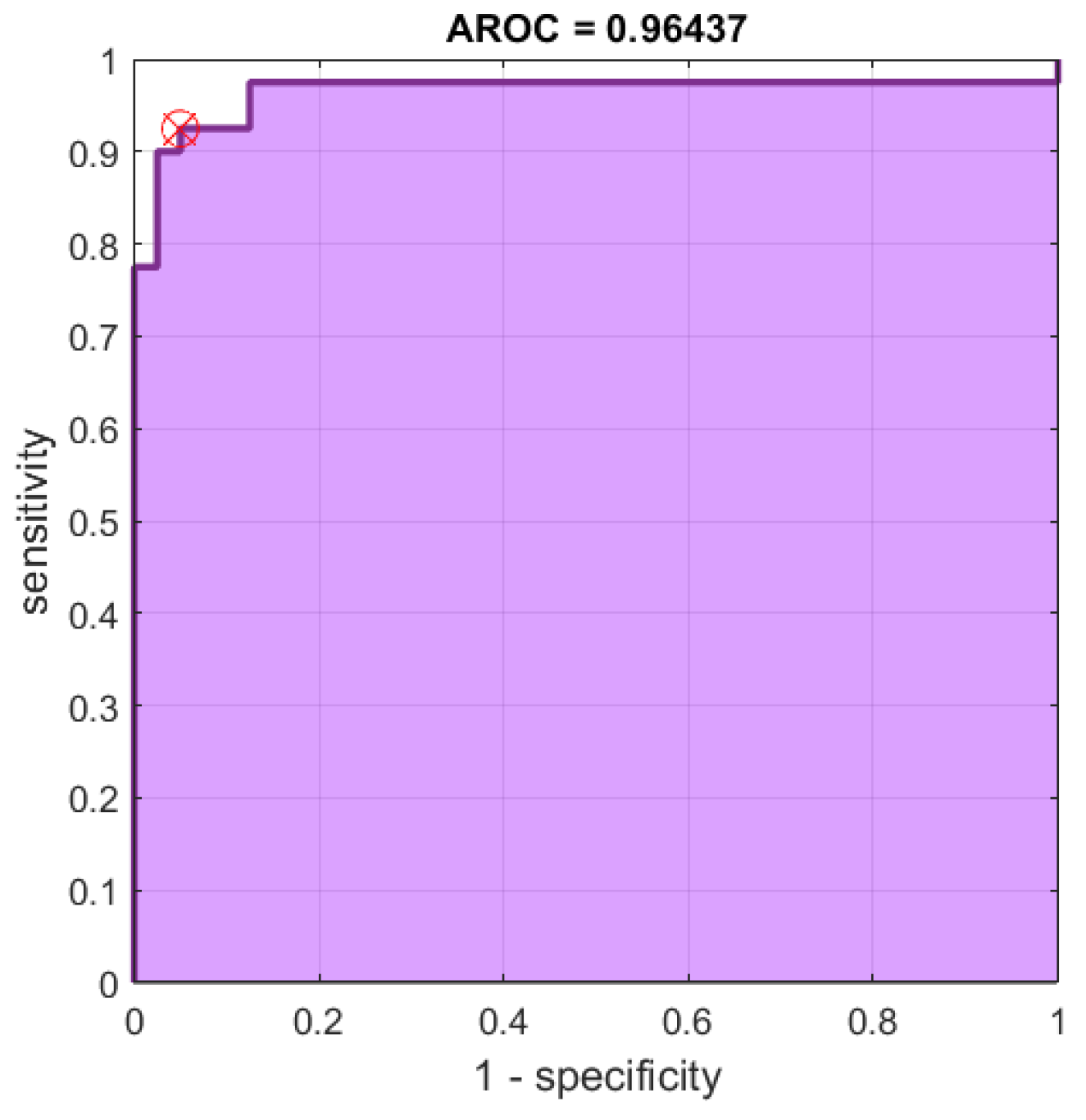
In addition to the p-value test, the receiver operating characteristic (ROC) and area under the ROC curve (AUC) of the results can be used as a criterion to measure the discrimination ability of our proposed measures. Since the best results (lowest p-values) were obtained for the RGB color space, we further establish the ROC curves for its , , and results, see Figure 16, Figure 17 and Figure 18, respectively. Moreover, the AUC, sensitivity, specificity, accuracy, and precision are shown for the RGB, HSV, and YUV color spaces in Table 4, Table 5 and Table 6, respectively. The results show that has high accuracy and AUC values for R, G, B, H, Y, U, and V channels. In addition, the multi-channel approaches ( and ) illustrate high accuracy and AUC values for the three color spaces. For the three proposed entropy measures, the best accuracy and AUC values were obtained for the RGB color space.
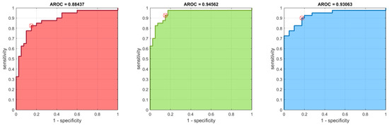
Figure 16.
ROC curves for results of the 40 melanoma and 40 melanocytic nevi images in the RGB color space. The curves are for , , and from left to right.

Figure 17.
ROC curves for results of the 40 melanoma and 40 melanocytic nevi images in the RGB color space.
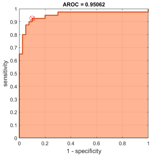
Figure 18.
ROC curves for results of the 40 melanoma and 40 melanocytic nevi images in the RGB color space.
Table 4.
ROC analysis for , , and results of 40 melanoma and 40 melanocytic nevi RGB images.
Table 5.
ROC analysis for , , and results of 40 melanoma and 40 melanocytic nevi HSV images.
Table 6.
ROC analysis for , , and results of 40 melanoma and 40 melanocytic nevi images in YUV.
Finally, we can say that the three entropy measures were able to differentiate both pigmented skin lesions. This was validated statistically by p-values, especially in the RGB color space. In the latter, achieved accuracies of 83.7%, 88.7%, 86.2% and AUC of 88.4%, 94.5%, 93%. On the other hand, , resulted in an accuracy of 93.7% and AUC of 96.4%. In addition, showed an accuracy of 91.2% and AUC of 95.0%.
5. Conclusions
In this paper, we presented a new concept and the first entropy method to investigate the single- and multi-channel features of colored images. To the best of our knowledge, this study is the only one that suggests entropy measures for analyzing colored images in their single- and multi-channel approaches. It was essential to perform some validation tests before employing those measures for analyzing colored medical images. The study was carried out as follows:
- Studying the sensitivity of the proposed measures to different initial parameters (tolerance level r and window size m).
- Identifying different irregularity degrees in colored images.
- Studying colored texture images in three color spaces.
- Analyzing medical images in three color spaces.
The three entropy measures, , , and , showed a reliable behavior with different initial parameters and an ability to gradually quantify irregularity degrees of colored textures and consistency upon repetition. When considering different color spaces, RGB, HSV, and YUV, these entropy measures showed promising results for the colored texture images.
Regarding the dermoscopic melanoma and melanocytic nevi images, single- and multi-channel entropy measures were able to differentiate both pigmented skin lesions. This was validated statistically by p-values, especially in the RGB color space. In the latter, achieved accuracies of 83.7%, 88.7%, 86.2% and AUC of 88.4%, 94.5%, 93%. On the other hand, , reached an accuracy of 93.7% and AUC of 96.4%. In addition, showed an accuracy of 91.2% and AUC of 95.0%. Moreover, and outperformed both and the classical descriptors, Haralick features, in differentiating the two similar malignant melanoma and benign melanocytic nevi dermoscopic images. These preliminary results could be the groundwork for developing an objective computer-based tool for helping medical doctors in diagnosing melanoma that is often mistaken for a benign melanocytic nevi or is properly diagnosed only in its late stages. We limited our investigation to three-channel colored images and, consequently, future work could be directed towards multi-spectral color images and towards more adapted applications for each color space and extending our study to a larger dataset.
Author Contributions
Conceptualization, M.H., A.H.-H. and A.S.G.; Methodology, M.H.; Software, M.H. and A.S.G.; Validation, M.H.; Formal Analysis, M.H., A.H.-H., A.S.G., P.G.V. and J.C.; Writing—Original Draft Preparation, M.H.; Writing—Review & Editing, M.H., A.H.-H., P.G.V., A.S.G. and J.C.; Visualization, M.H.; Supervision, A.H.-H. and M.H. All authors have read and agreed to the published version of the manuscript.
Funding
This research received no external funding.
Institutional Review Board Statement
Not applicable.
Informed Consent Statement
Not applicable.
Data Availability Statement
Data sharing not applicable.
Conflicts of Interest
The authors declare no conflict of interest.
References
- Humeau-Heurtier, A. Texture feature extraction methods: A survey. IEEE Access 2019, 7, 8975–9000. [Google Scholar] [CrossRef]
- Song, T.; Feng, J.; Wang, S.; Xie, Y. Spatially weighted order binary pattern for color texture classification. Expert Syst. Appl. 2020, 147, 113167. [Google Scholar] [CrossRef]
- Liu, L.; Chen, J.; Fieguth, P.; Zhao, G.; Chellappa, R.; Pietikäinen, M. From BoW to CNN: Two decades of texture representation for texture classification. Int. J. Comput. Vis. 2019, 127, 74–109. [Google Scholar] [CrossRef] [Green Version]
- Liu, L.; Fieguth, P.; Guo, Y.; Wang, X.; Pietikäinen, M. Local binary features for texture classification: Taxonomy and experimental study. Pattern Recognit. 2017, 62, 135–160. [Google Scholar] [CrossRef] [Green Version]
- Nguyen, T.P.; Vu, N.S.; Manzanera, A. Statistical binary patterns for rotational invariant texture classification. Neurocomputing 2016, 173, 1565–1577. [Google Scholar] [CrossRef]
- Qi, X.; Zhao, G.; Shen, L.; Li, Q.; Pietikäinen, M. LOAD: Local orientation adaptive descriptor for texture and material classification. Neurocomputing 2016, 184, 28–35. [Google Scholar] [CrossRef] [Green Version]
- Wang, S.; Wu, Q.; He, X.; Yang, J.; Wang, Y. Local N-Ary pattern and its extension for texture Classification. IEEE Trans. Circuits Syst. Video Technol. 2015, 25, 1495–1506. [Google Scholar] [CrossRef]
- Zhang, J.; Liang, J.; Zhang, C.; Zhao, H. Scale invariant texture representation based on frequency decomposition and gradient orientation. Pattern Recognit. Lett. 2015, 51, 57–62. [Google Scholar] [CrossRef]
- Backes, A.R.; Martinez, A.S.; Bruno, O.M. Texture analysis using graphs generated by deterministic partially self-avoiding walks. Pattern Recognit. 2011, 44, 1684–1689. [Google Scholar] [CrossRef]
- Ghalati, M.K.; Nunes, A.; Ferreira, H.; Serranho, P.; Bernardes, R. Texture analysis and its applications in biomedical imaging: A survey. IEEE Rev. Biomed. Eng. 2021, 15, 222–246. [Google Scholar] [CrossRef]
- Yeh, J.R.; Lin, C.W.; Shieh, J.S. An approach of multiscale complexity in texture Analysis of lymphomas. IEEE Signal Process. Lett. 2011, 18, 239–242. [Google Scholar] [CrossRef]
- Silva, L.; Senra Filho, A.; Fazan, V.P.S.; Felipe, J.C.; Junior, L.M. Two-dimensional sample entropy: Assessing image texture through irregularity. Biomed. Phys. Eng. Express 2016, 2, 045002. [Google Scholar] [CrossRef]
- Dos Santos, L.F.S.; Neves, L.A.; Rozendo, G.B.; Ribeiro, M.G.; do Nascimento, M.Z.; Tosta, T.A.A. Multidimensional and fuzzy sample entropy (SampEnMF) for quantifying H&E histological images of colorectal cancer. Comput. Biol. Med. 2018, 103, 148–160. [Google Scholar]
- Azami, H.; Escudero, J.; Humeau-Heurtier, A. Bidimensional distribution entropy to analyze the irregularity of small-sized textures. IEEE Signal Process. Lett. 2017, 24, 1338–1342. [Google Scholar] [CrossRef] [Green Version]
- Silva, L.E.; Duque, J.J.; Felipe, J.C.; Murta Jr, L.O.; Humeau-Heurtier, A. Two-dimensional multiscale entropy analysis: Applications to image texture evaluation. Signal Process. 2018, 147, 224–232. [Google Scholar] [CrossRef]
- Humeau-Heurtier, A.; Omoto, A.C.M.; Silva, L.E. Bi-dimensional multiscale entropy: Relation with discrete Fourier transform and biomedical application. Comput. Biol. Med. 2018, 100, 36–40. [Google Scholar] [CrossRef]
- Hilal, M.; Berthin, C.; Martin, L.; Azami, H.; Humeau-Heurtier, A. Bidimensional Multiscale Fuzzy Entropy and its application to pseudoxanthoma elasticum. IEEE Trans. Biomed. Eng. 2019, 67, 2015–2022. [Google Scholar] [CrossRef]
- Furlong, R.; Hilal, M.; O’brien, V.; Humeau-Heurtier, A. Parameter Analysis of Multiscale Two-Dimensional Fuzzy and Dispersion Entropy Measures Using Machine Learning Classification. Entropy 2021, 23, 1303. [Google Scholar] [CrossRef]
- Palm, C. Color texture classification by integrative co-occurrence matrices. Pattern Recognit. 2004, 37, 965–976. [Google Scholar] [CrossRef]
- Backes, A.R.; Casanova, D.; Bruno, O.M. Color texture analysis based on fractal descriptors. Pattern Recognit. 2012, 45, 1984–1992. [Google Scholar] [CrossRef]
- Drimbarean, A.; Whelan, P.F. Experiments in colour texture analysis. Pattern Recognit. Lett. 2001, 22, 1161–1167. [Google Scholar] [CrossRef] [Green Version]
- Xu, Q.; Yang, J.; Ding, S. Color texture analysis using the wavelet-based hidden Markov model. Pattern Recognit. Lett. 2005, 26, 1710–1719. [Google Scholar] [CrossRef]
- Arvis, V.; Debain, C.; Berducat, M.; Benassi, A. Generalization of the cooccurrence matrix for colour images: Application to colour texture classification. Image Anal. Stereol. 2004, 23, 63–72. [Google Scholar] [CrossRef] [Green Version]
- Alata, O.; Burie, J.C.; Moussa, A.; Fernandez-Maloigne, C.; Qazi, I.-U.-H. Choice of a pertinent color space for color texture characterization using parametric spectral analysis. Pattern Recognit. 2011, 44, 16–31. [Google Scholar]
- Mäenpää, T.; Pietikäinen, M. Classification with color and texture: Jointly or separately? Pattern Recognit. 2004, 37, 1629–1640. [Google Scholar] [CrossRef] [Green Version]
- Bianconi, F.; Harvey, R.W.; Southam, P.; Fernández, A. Theoretical and experimental comparison of different approaches for color texture classification. J. Electron. Imaging 2011, 20, 043006. [Google Scholar] [CrossRef]
- Manjunath, B.S.; Ohm, J.R.; Vasudevan, V.V.; Yamada, A. Color and texture descriptors. IEEE Trans. Circuits Syst. Video Technol. 2001, 11, 703–715. [Google Scholar] [CrossRef] [Green Version]
- Hilal, M.; Gaudêncio, A.S.F.; Berthin, C.; Vaz, P.G.; Cardoso, J.a.; Martin, L.; Humeau-Heurtier, A. Bidimensional Colored Fuzzy entropy measure: A Cutaneous Microcirculation Study. In Proceedings of the Fifth International Conference on Advances in Biomedical Engineering (ICABME), Tripoli, Lebanon, 17–19 October 2019. [Google Scholar]
- Celebi, M.E.; Codella, N.; Halpern, A. Dermoscopy image analysis: Overview and future directions. IEEE J. Biomed. Health Inform. 2019, 23, 474–478. [Google Scholar] [CrossRef]
- Talavera-Martínez, L.; Bibiloni, P.; González-Hidalgo, M. Computational Texture Features of Dermoscopic Images and Their Link to the Descriptive Terminology—A Survey. Comput. Methods Programs Biomed. 2019, 182, 105049. [Google Scholar] [CrossRef]
- Barata, C.; Celebi, M.E.; Marques, J.S. A survey of feature extraction in dermoscopy image analysis of skin cancer. IEEE J. Biomed. Health Inform. 2018, 23, 1096–1109. [Google Scholar] [CrossRef]
- Machado, M.; Pereira, J.; Fonseca-Pinto, R. Classification of reticular pattern and streaks in dermoscopic images based on texture analysis. J. Med. Imaging 2015, 2, 044503. [Google Scholar] [CrossRef] [PubMed] [Green Version]
- Garnavi, R.; Aldeen, M.; Bailey, J. Computer-aided diagnosis of melanoma using border-and wavelet-based texture analysis. IEEE Trans. Inf. Technol. Biomed. 2012, 16, 1239–1252. [Google Scholar] [CrossRef] [PubMed]
- Sáez, A.; Acha, B.; Serrano, A.; Serrano, C. Statistical detection of colors in dermoscopic images with a texton-based estimation of probabilities. IEEE J. Biomed. Health Inform. 2018, 23, 560–569. [Google Scholar] [CrossRef] [PubMed]
- Isasi, A.G.; Zapirain, B.G.; Zorrilla, A.M. Melanomas non-invasive diagnosis application based on the ABCD rule and pattern recognition image processing algorithms. Comput. Biol. Med. 2011, 41, 742–755. [Google Scholar] [CrossRef]
- Celebi, M.E.; Zornberg, A. Automated quantification of clinically significant colors in dermoscopy images and its application to skin lesion classification. IEEE Syst. J. 2014, 8, 980–984. [Google Scholar] [CrossRef]
- Celebi, M.E.; Kingravi, H.A.; Uddin, B.; Iyatomi, H.; Aslandogan, Y.A.; Stoecker, W.V.; Moss, R.H. A methodological approach to the classification of dermoscopy images. Comput. Med. Imaging Graph. 2007, 31, 362–373. [Google Scholar] [CrossRef] [Green Version]
- Hilal, M.; Humeau-Heurtier, A. Bidimensional fuzzy entropy: Principle analysis and biomedical applications. In Proceedings of the 2019 41st Annual International Conference of the IEEE Engineering in Medicine and Biology Society (EMBC), Berlin, Germany, 23–27 July 2019; pp. 4811–4814. [Google Scholar]
- Chen, W.; Wang, Z.; Xie, H.; Yu, W. Characterization of surface EMG signal based on fuzzy entropy. IEEE Trans. Neural. Syst. Rehabil. Eng. 2007, 15, 266–272. [Google Scholar] [CrossRef]
- Gaudêncio, A.S.F.; Vaz, P.G.; Hilal, M.; Cardoso, J.M.; Mahé, G.; Lederlin, M.; Humeau-Heurtier, A. Three-dimensional multiscale fuzzy entropy: Validation and application to idiopathic pulmonary fibrosis. IEEE J. Biomed. Health Inform. 2020, 25, 100–107. [Google Scholar] [CrossRef]
- Abdelmounaime, S.; Dong-Chen, H. New Brodatz-based image databases for grayscale color and multiband texture analysis. ISRN Mach. Vis. 2013, 2013, 876386. [Google Scholar] [CrossRef]
- Colored Brodatz Texture. Available online: http://multibandtexture.recherche.usherbrooke.ca/ (accessed on 10 June 2022).
- Haralick, R.M.; Shanmugam, K.; Dinstein, I.H. Textural features for image classification. IEEE Trans. Syst. Man Cybern. Syst. 1973, SMC-3, 610–621. [Google Scholar] [CrossRef] [Green Version]
- Philips, C.; Li, D.; Raicu, D.; Furst, J. Directional invariance of co-occurrence matrices within the liver. In Proceedings of the 2008 International Conference on Biocomputation, Bioinformatics, and Biomedical Technologies, Bucharest, Romania, 29 June–5 July 2008; pp. 29–34. [Google Scholar]
- Tschandl, P.; Rosendahl, C.; Kittler, H. The HAM10000 dataset, a large collection of multi-source dermatoscopic images of common pigmented skin lesions. Sci. Data 2018, 5, 180161. [Google Scholar] [CrossRef] [PubMed]
- Tschandl, P. Replication data for: “The HAM10000 Dataset, a larGe Collection of Multi-source Dermatoscopic Images of comMon Pigmented Skin Lesions”. Harvard Dataverse, V3, UNF:6:/APKSsDGVDhwPBWzsStU5A==. 2018. Available online: https://dataverse.harvard.edu/dataset.xhtml?persistentId=doi:10.7910/DVN/DBW86T (accessed on 10 June 2022).
- Sawilowsky, S.S. New effect size rules of thumb. J. Mod. Appl. Stat. Methods 2009, 8, 26. [Google Scholar] [CrossRef]
- Cohen, J. Statistical Power Analysis for the Behavioral Sciences; Routledge: London, UK, 2013. [Google Scholar]


Publisher’s Note: MDPI stays neutral with regard to jurisdictional claims in published maps and institutional affiliations. |
© 2022 by the authors. Licensee MDPI, Basel, Switzerland. This article is an open access article distributed under the terms and conditions of the Creative Commons Attribution (CC BY) license (https://creativecommons.org/licenses/by/4.0/).