In this section, we will respectively apply the traditional K-means, GMM and the SKM algorithm on the processed data. By analyzing the cluster results and calculating the assessment criteria scores, we can compare the performance of different algorithms as well as give the academic levels of the 20 universities. The estimation of university academic level is given by the most reasonable cluster result, as all these cluster algorithms evolve random processes.
5.1. The K-Means Algorithm Clustering
To avoid the influence of sparse data and speed up the process of convergence, PCA is used at first to reduce the data dimension [
27]. The PCA scree plot is displayed as
Figure 1.
Often, there are two ways to obtain the number of principal components, that is, to retain a certain percentage of the variance of the original data or to retain only the principal components with eigenvalues greater than 1 according to Kraiser’s rule [
28,
29]. It can be seen in the shown PCA results that there are five principal components with eigenvalues greater than 1, and when the number of principal components is 6, the cumulative variance contribution rate reaches more than 0.8. We finally choose to keep six principal components, that is, compress the 32-dimension original data to six dimensions. It is worth mentioning that several indicators ignored in previous research prove to contribute signficantly according to the PCA results, which are shown above. This is a strong testament to the effectiveness of big data.
There are many methods for deciding the number of clusters
K. One simple way is to observe the sum of the squarred errors (SSE) with the change of
K and select the point where SSE changes from steep to gentle. However, the
Figure 2 shows that there is no very clear elbow point. As a consequence, we choose to use the Gap Statistic method [
30]. Every
K corresponds to a
and
, and
K is selected as the minimal
K that makes
. We conduct simulations 50 times, as random sampling is also used in the Gap Statistic. The results are shown in
Figure 3, and
Figure 4 shows the most common case. It can be seen that when
, the GapDiffs are most likely to be greater than 0. Although inferior to
,
also shows a considerable frequency. Considering that academic performance evaluation needs an adequate
K to produce reasonable results, we finally chose
K as 4, 5 and 6.
In order to obtain credible results, we limit the iteration times of each simulation to 20, so as to avoid bad cases caused by random initialization. In addition, we merge those simulations that have very similar initialization and cluster results. We select the most representive case by comparing their clustering evaluation criteria [
31,
32]. This strategy makes it easier for us to analyze the performance of different algorithms. For eack
K, we conduct 30 independent simulations and give the cluster details. To better visualize the clusters, we map the original data points to a plane using PCA. The results are shown in the table and graph below.
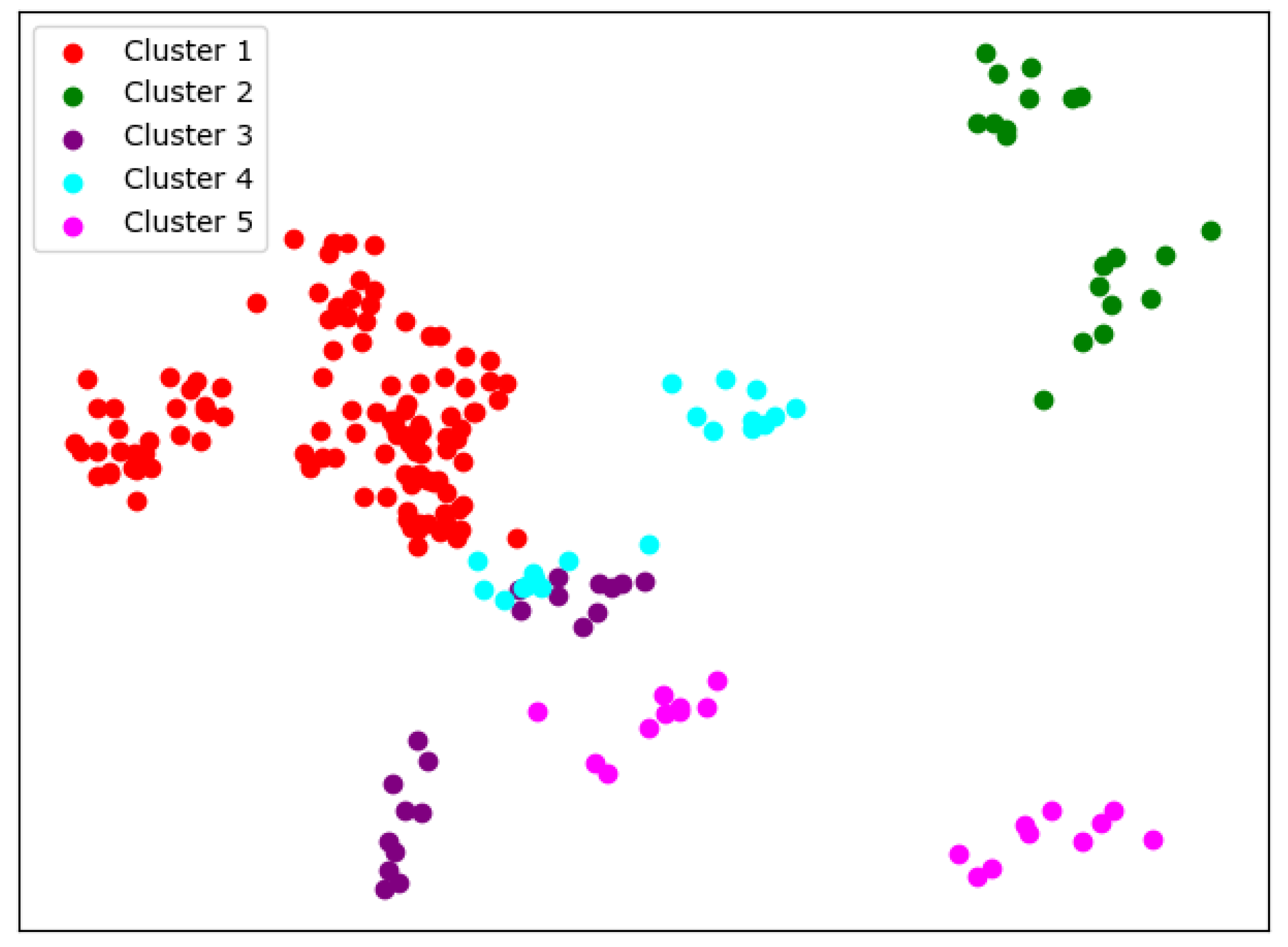
When
, we can see from
Figure 5 that the cluster completeness is well preserved. Only Xi’an Jiaotong University and Tongji University have small parts divided into different clusters, and the rest of the data points of the same university are all in the same cluster.
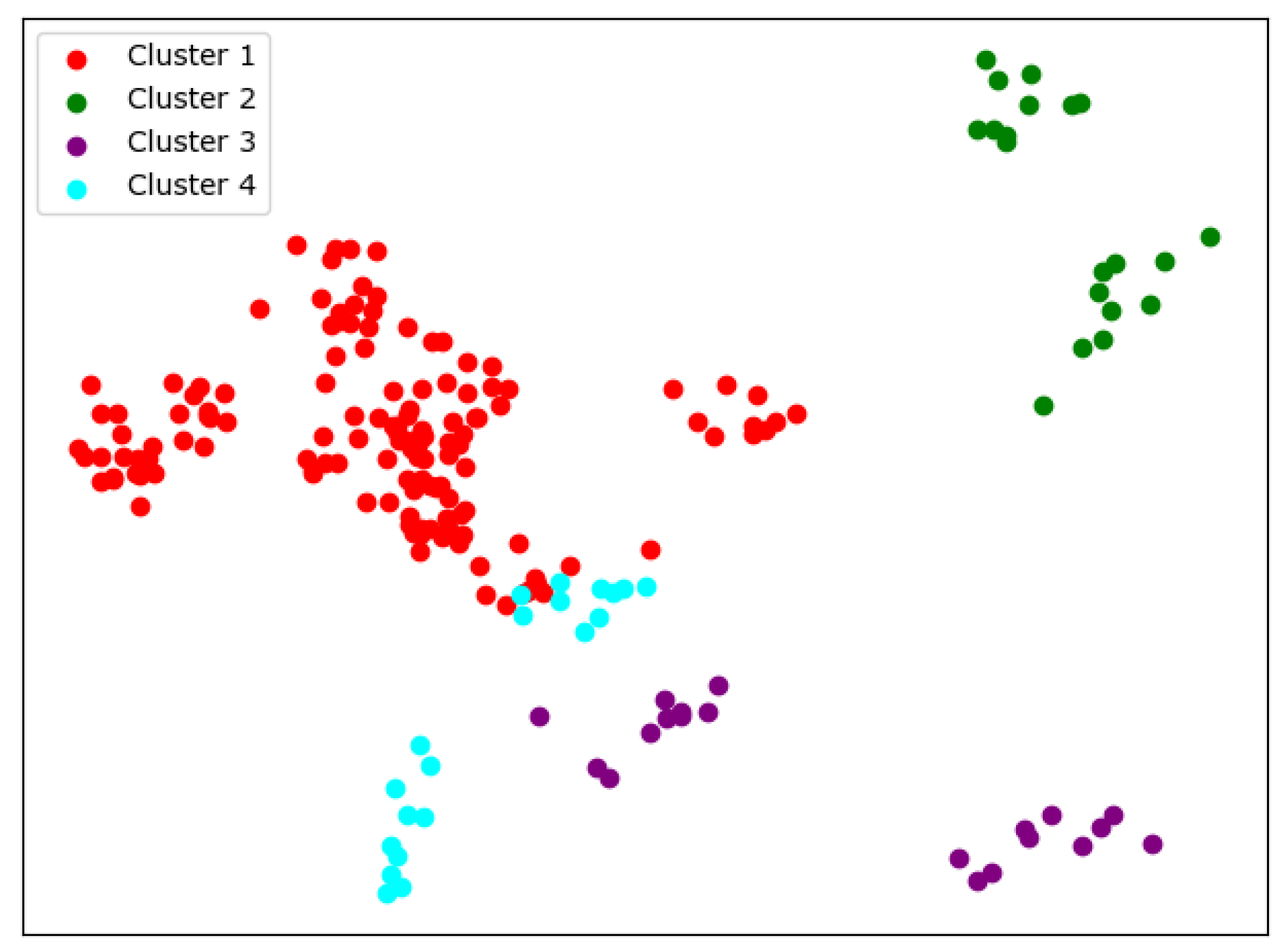
When
, the cluster result
Figure 6 still shows very good completeness. However, some universities have changed from one cluster to another. Peking University itself becomes one new cluster, and Wuhan University becomes clustered with Beijing Normal University and Fudan University.
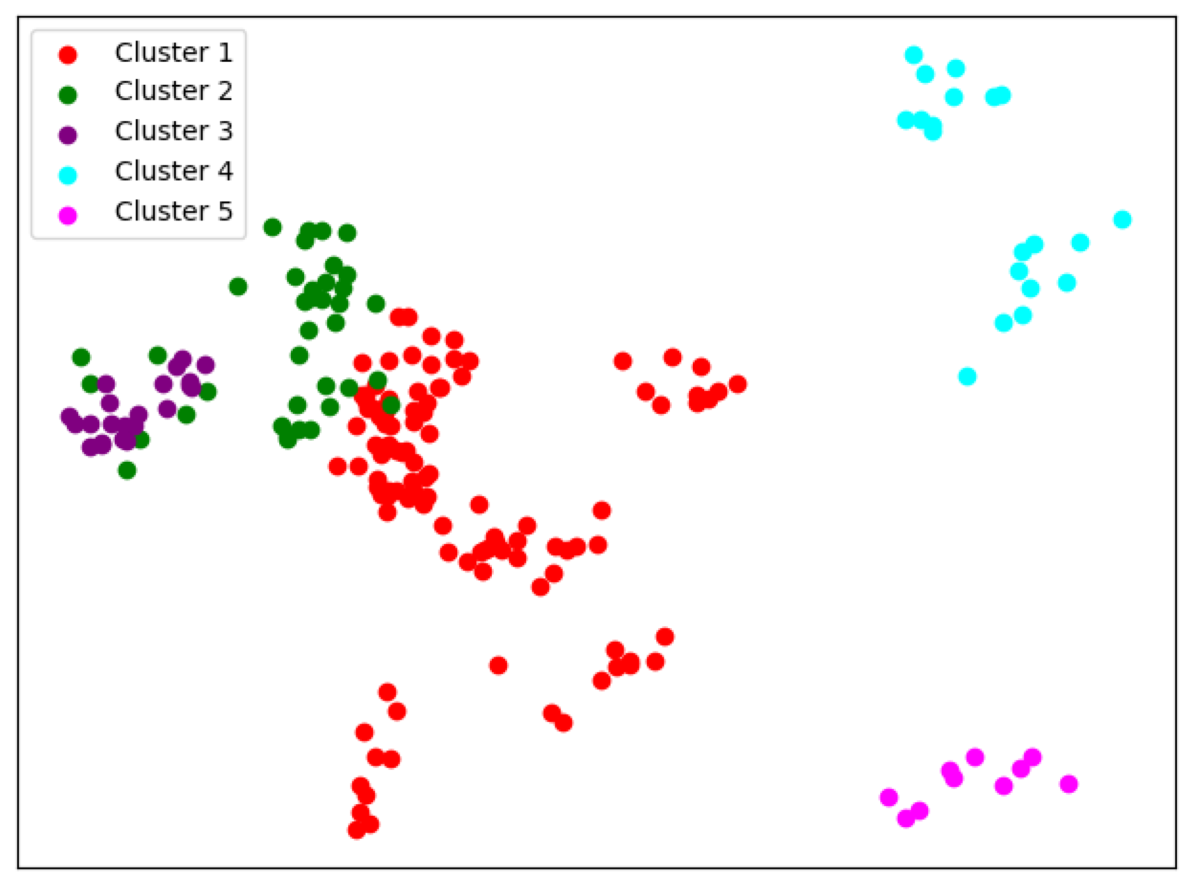
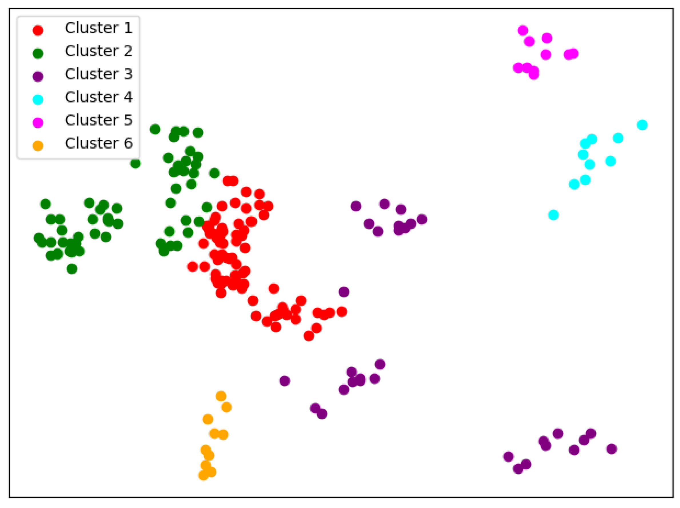
When
, things begin to change. We can see from
Figure 7 that so-called rag bags, which mean small parts of data points that cannot be well clustered, begin to increase. This actually has a bad effect on the cluster homogenity. Shanghai Jiao Tong University and Sun Yat-sen University now also change the cluster and join with Fudan University, while Wuhan University and Beijing Normal University remain together.
It can be seen from
Table 3 that the clustering indicators of the K-means algorithm are relatively stable. DBI is basically maintained between 1.3 and 1.6, DI is basically maintained between 0.05 and 0.08, and SC is mostly distributed above 0.3. It is in line with the previous SSE result and proves the cluster result to be reasonable. For results, with the change of
K, the data points of Tsinghua University and Zhejiang University in all years are always the only two in the same cluster, which indicates that the academic level of these two universities is very close and there is a large gap between the two and the remaining universities. In addition, in all years data points of Central South University, Jilin University, Sichuan University, Huazhong University of Science and Technology, Shandong University, Tongji University, etc. always appear in the same cluster, indicating their academic level is close; Northwestern Polytechnical University, Beihang University, Beijing Institute of Technology, Harbin Institute of Technology and Southeast University are in the same situation, and the difference between these two clusters may be that the universities in the latter cluster have a strong color of science and engineering along with a national defense background. Considering that Xi’an Jiaotong University has a relatively uniform distribution in the two clusters with the change of
K, it is likely that the academic level is close. We also notice that the clustering results of Wuhan University, Sun Yat-sen University, Fudan University, Shanghai Jiao Tong University, Beijing Normal University, Peking University and other universites changed greatly with the change of
K. When
, Beijing Normal University and Peking University are in the same cluster, but it is then divided as
K increases. One explanation is that when
K is small, Beijing Normal University and Peking University are clustered together because they have similar backgrounds in humanities and social sciences. However, because of the huge difference of academic level, the two are then divided. This also explains the cluster variance for Fudan University, Sun Yat-sen University, Wuhan University, and Shanghai Jiao Tong University. These are all comprehensive universities, and characteristics of both (1) humanities and social science and (2) science and engineering are relatively distinct. Therefore, for different
K, they can be in the same cluster with Beijing Normal University or in the cluster of science and engineering backgrounds.
5.3. The SKM Algorithm Clustering
The idea of the SKM algorithm is based on the assumption that in the original data point cloud, the neighborhood of each point should have a convergent property with this point. The point cloud is the sampling and discretization of real physical quantities, so the rationality of this assumption is quite natural. In our simulation, we firstly use the k-nearest neighbor method to select points near each data point and map this subcloud to an N-dimensional normal distribution family manifold. Then, we apply the SKM algorithm with non-Euclidean difference functions and analyze their clustering results. For the selection of k, we simply choose , which is the number of the points in the origin point cloud for every university. The choice not only enables the points from the same university to be mapped to one distribution on statistical manifolds in theory: it also has been proven in our simulation that when , the SKM algorithm could achieve convergence faster compared to other k-values.
In this simulation, we use the KL divergence and the Wasserstein difference functions. Due to the use of the local statistical method, there is no need for dimension reduction; in other words, the application of PCA is skipped. Especially, as there is a one-to-one correspondence between the point clouds on Euclidean space and on manifolds, and in the Euclidean space we have obtained
K values, we just keep it unchanged as our simulation parameters [
34]. The other simulation strategies are the same as those in
Section 4.1. The results are shown in the table and graph below.
The first is the result of using KL divergence.
When
, we can see similar results with K-means from
Figure 12; the cluster completeness is also well preserved. However, this time, Peking University is divided into a separate cluster, and Beijing Normal University is divided into a large cluster.
Compared with K-means, we can see from
Figure 13 that the biggest difference when
is that this time, Sun Yat-sen University, Fudan University, and Shanghai Jiao Tong University are in the same cluster. Except for Peking University, Zhejiang University, and Tsinghua University, the rest are divided into two main clusters.
When
, it also fails to cluster a small number of data points well. In
Figure 14, Peking University, Tsinghua University, and Zhejiang University were each divided into a cluster.
The result for the Wasserstein distance is below.
When
, we can see from
Figure 15 that the difference between using Wasserstein distance and KL divergence is that when using Wasserstein distance, Fudan University is divided into the same cluster as Peking University. The rest of the results are basically the same.
When
, the SKM results in
Figure 16 are basically the same with using Wasserstein distance and KL divergence, but with using KL divergence, it is more likely that small parts of data points cannot be well clustered.
When
, the clustering results with using Wasserstein distance in
Figure 17 are less stable relative to KL divergence. In addition, the Wasserstein distance produce clusters with a very small number of samples, which indicates that it cannot distinguish the mainfolds on this problem very well.
We can see from
Table 5 and
Table 6 that the SKM algorithm is inferior to the K-means and GMM method on the two indicators of DBI and DI. From the definitions of DBI and DI, we speculate that this can be caused by the local statistical methods. During the process of selecting a local point cloud, we use the K-nearest neighbor strategy. It can better reflect the statistical density characteristics of a local point cloud, but on the other hand, it may also cause the selected area to be non-convex, resulting in a diffrent distribution in parameter space from the original space. However, the SC indicator of both metrics for the SKM algorithm performs better than that in K-means and GMM. We attribute this to the introduction of non-Euclidean metrics, which achieve a more granular comparison. It can also be seen from the degree of dispersion of the statistical indicators that the two indicators in this section fluctuate considerably, as the selection of the initial cluster center will greatly affect the final clustering, which is a manifestation of the high sensitivity of the SKM algorithm. Between the two metric functions of the SKM algorithm, the KL divergence performs better, as it gives more stable results and better interpretability, while the Wasserstein distance has greatly varied indicators and gives clusters of high similarities.
In terms of clustering results, the clusters given by the SKM algorithm are generally similar to the results of K-means and general cases of GMM, and they actually have better discrimination on the universities of science and technology than the other case of GMM, but there are still some interesting phenomena. After verification and comparison, it can be seen that using several Riemann metrics defined on symmetric positive definite manifolds, the obtained clustering effect is not as good as KL divergence. Hence, we choose KL divergence as the distance function for clustering. In the results of KL divergence, the clustering results are relatively more stable and have no university spans from one cluster to another. The biggest difference is that the KL divergence does not give a division among comprehensive universities; instead, it further divides universities of science and engineering, resulting in the cluster of Peking University, Beihang University and Northwestern Polytechnical University as well as Harbin Institute of Technology, Southeast University, Xi’an Jiaotong University. As for Wasserstein distance, it has unsatifactory indicators and results. Especially when , the Wasserstein metric produce clusters with a very small number of samples, which indicates that it cannot distinguish the mainfolds on this problem very well. It is worth noting that the dimension of the data on which the SKM algorithm is applied is 32 compared to six for the traditional K-means and GMM algorithms. In this case, the SKM algorithm still obtains remarkable clustering results, which proves the potential of the SKM algorithm in terms of processing large amounts of high-dimensional data.
To further assess the three algorithms quantitatively, we apply them on a UCI ML dataset [
35] and compare the accuracies. We choose to use the ’Steel Plates Faults Data Set’ provided by Semeion from the Research Center of Sciences of Communication, Via Sersale 117, 00128, Rome, Italy. Every sample in the dataset consists of 27 features, and the task is to classify whether a sample has any of the seven faults. We choose this dataset because it has similar feature dimensions with our origin problem and it provides various indicators to classify, which can better assess the different clustering algorithms. The results are produced under the same condition as the simulation set above, including data pre-processing methods and cluster parameters. The classification accuracies of different algorithms on the seven faults are shown in
Table 7.
We can see that the SKM algorithm is greatly advantageous over the K-means and the GMM algorithm on accuracy scores. In comparison, the dataset provider’s model has an average accuracy of 0.77 on this dataset [
36]. In addition, in terms of cluster indicators, we can see from
Table 8 that the SKM algorithm has better performance on the SC score, but it does not perform well on the DBI score, which is basically consistent with the results on the Chinese University dataset. The result exactly reveals the great potential of the SKM algorithm on the application of many other fields. It could be a great replacement of traditional Euclidean-based cluster methods in a certain problem.


