
Deep Image Steganography Using Transformer and Recursive Permutation


Abstract
:1. Introduction
2. Related Works
2.1. Image Encryption
2.2. Image Steganography
2.3. Deep Learning
2.4. Transformer
2.5. Motivation
3. TRPSteg: Transformer and Recursive Permutation-Based Image Steganography
3.1. Recursive Permutation
| Algorithm 1 Recursion_encryption(img, width, height, S) |
| Input: The secret image to encrypt, img; The width of image, width; The height of image, height; The generated chaotic sequence, S; |
| Output: The encrypted image, img; |
| nw ←⌊width/2⌋, nh ←⌊height/2⌋ |
| if nw < 1 or nh < 1 then |
| return img |
| else |
| //Divide the image into four parts, and encrypt the four parts, respectively. Encrypt the upper left part. |
| Recursion_encryption(img[0:nw, 0:nh, :], nw, nh, S) |
| //Use the logistic_scramble_encryption function (Algorithm 2) to scramble the image with the chaotic sequence generated by the logistic algorithm. |
| img[0:nw, 0:nh] ← logistic_scramble_encryption(img[0:nw, 0:nh], S) |
| //Encrypt the lower left part. |
| Recursion_encryption(img[0:nw, nh:height], nw, nh, S) |
| img[0:nw, nh: height] ← logistic_scramble_encryption(img[0:nw, nh: height], S) |
| //Encrypt the upper right part. |
| Recursion_encryption(img[nw:width, 0:nh], nw, nh, S) |
| img[nw:width, 0:nh] ← logistic_scramble_encryption(img[nw:width, 0:nh], S) |
| //Encrypt the lower right part. |
| Recursion_encryption(img[nw:width, nh:height], nw, nh, S) |
| img[nw:width, nh:height] ← logistic_scramble_encryption(img[nw:width, |
| nh:height], S) |
| //Encrypt the entire image. |
| img[0:width, 0:height] ← logistic_scramble_encryption(img[0:width, 0:height], S) |
| end if |
| return img |
| Algorithm 2 logistic _scramble_encryption(img, S) |
| Input: The image to encrypt, img; The generated chaotic sequence, S; |
| Output: The encrypted image, img; |
| w, h ← img.shape //Get the width (w) and height (h) of img. |
| img ← img.flatten() //Convert img to 1D array. |
| idx ← sort(S) //Sort S to obtain the corresponding indices (idx) of S. |
| img ← img[idx,:] |
| img ← img.reshape(w,h,3) |
| return img |
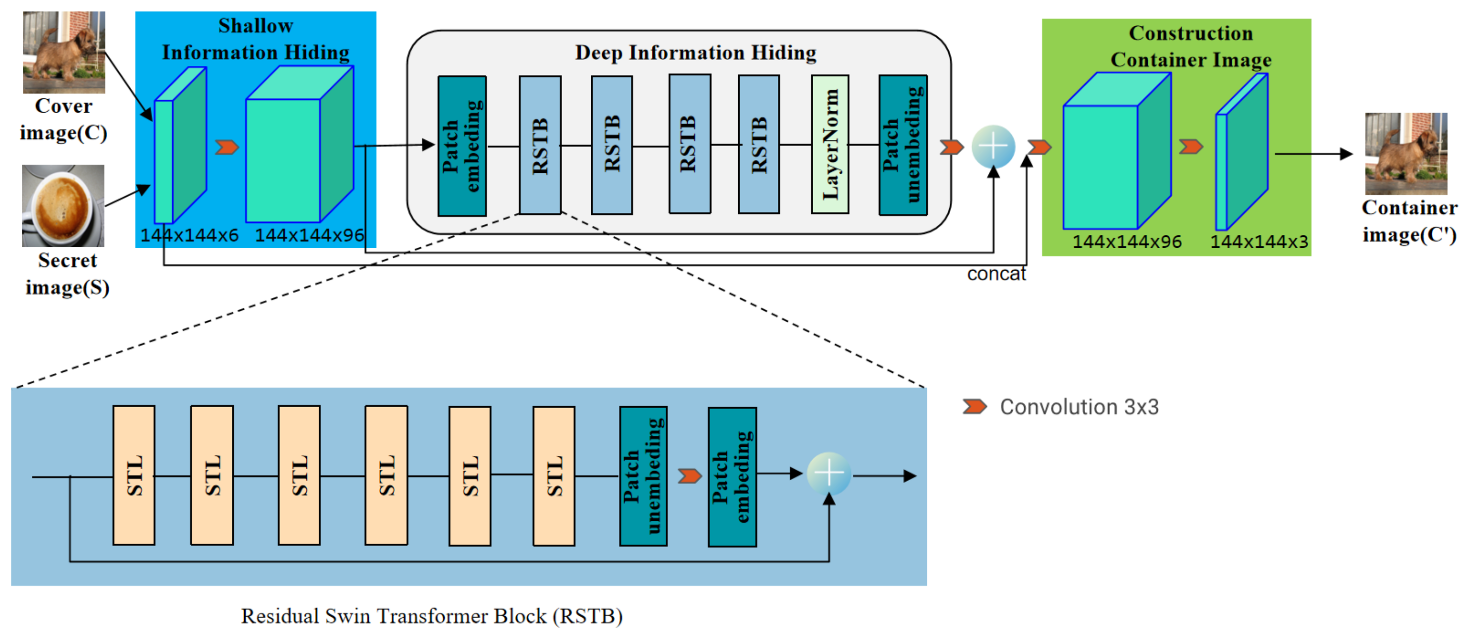
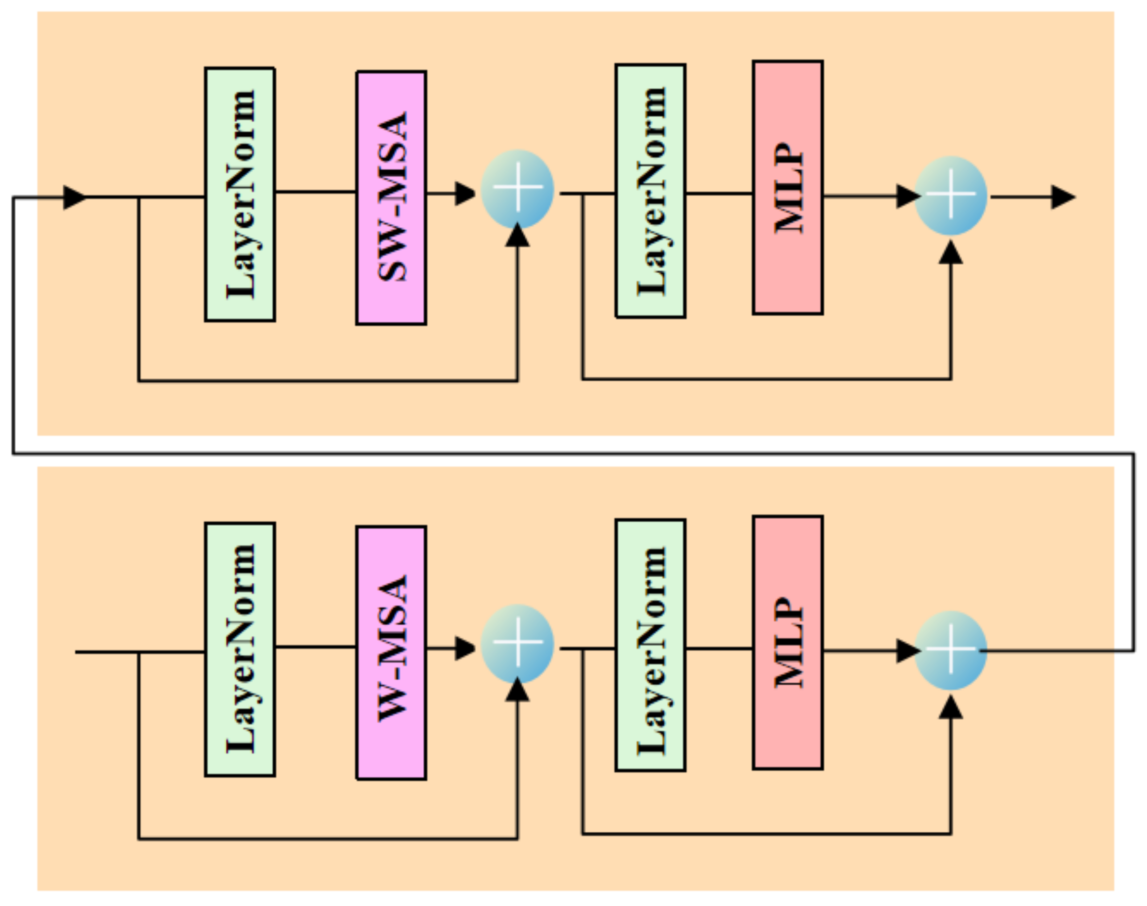
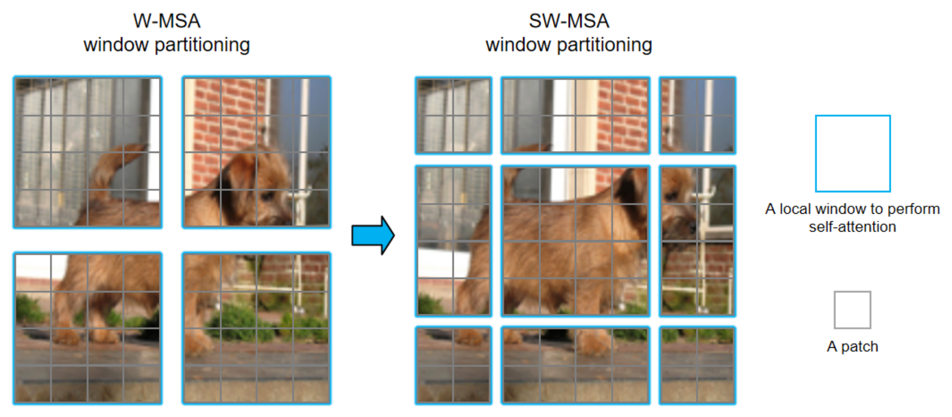
3.2. Hiding Network
3.3. Extraction Network
3.4. Loss Function
3.5. Flowchart
3.6. Differences between TRPSteg and Other Image Steganography Schemes
4. Experiments
4.1. Experimental Setting
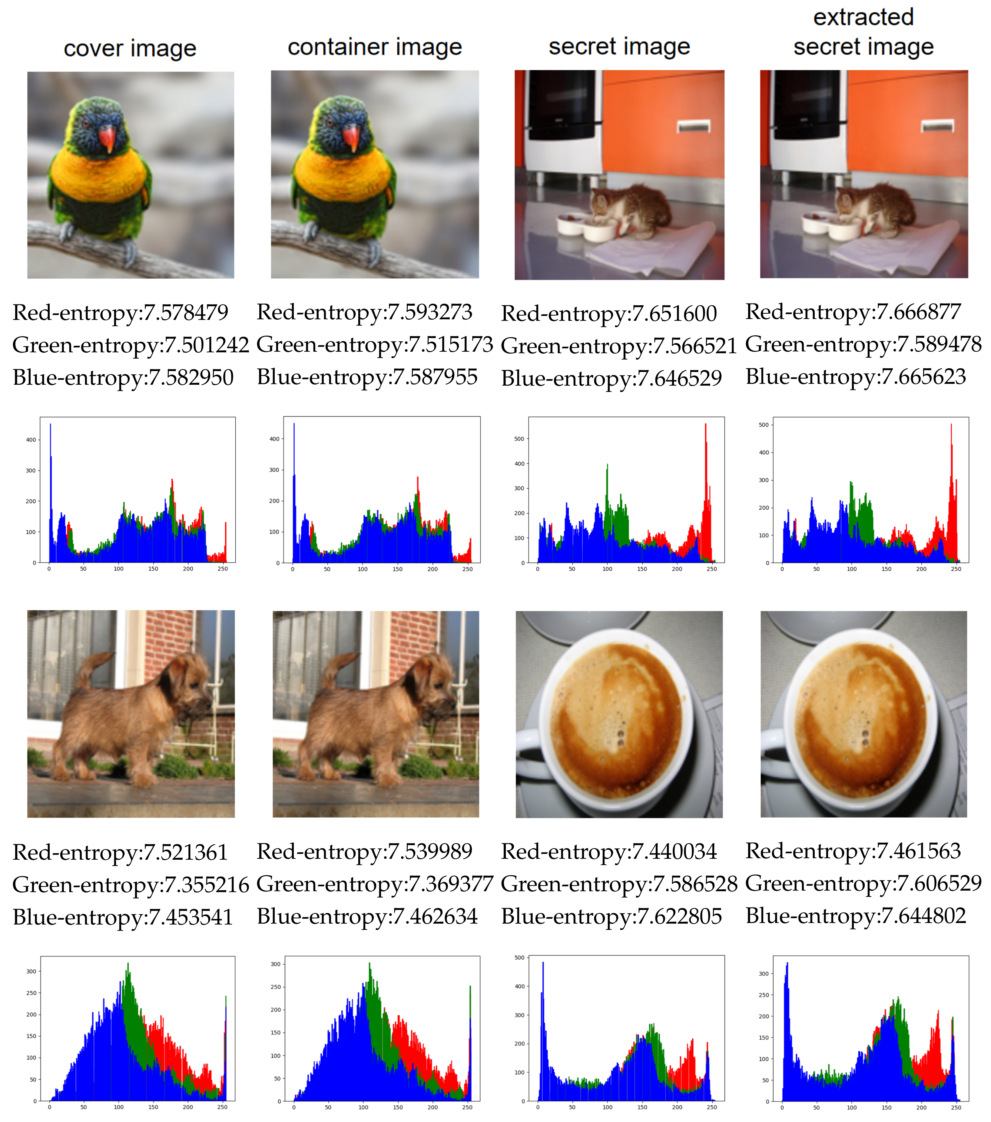
4.2. Visual Effect
4.3. Security Analysis
4.4. Image Quality
4.5. Hidden Capacity Analysis
4.6. Parameter Influence and Ablation Study
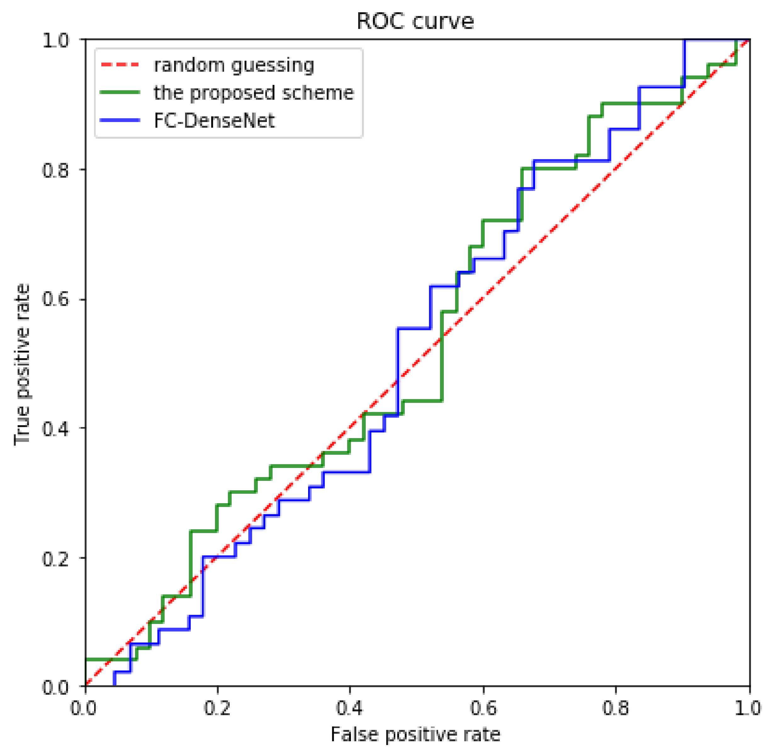
4.7. Statistical Test
4.8. Threats to Validity
4.9. Discussion
5. Conclusions
Author Contributions
Funding
Institutional Review Board Statement
Informed Consent Statement
Data Availability Statement
Conflicts of Interest
References
- Mohanarathinam, A.; Kamalraj, S.; Prasanna Venkatesan, G.; Ravi, R.V.; Manikandababu, C. Digital watermarking techniques for image security: A review. J. Ambient. Intell. Humaniz. Comput. 2020, 11, 3221–3229. [Google Scholar] [CrossRef]
- Li, T.; Zhang, D. Hyperchaotic Image Encryption Based on Multiple Bit Permutation and Diffusion. Entropy 2021, 23, 510. [Google Scholar] [CrossRef] [PubMed]
- Subramanian, N.; Elharrouss, O.; Al-Maadeed, S.; Bouridane, A. Image steganography: A review of the recent advances. IEEE Access 2021, 11, 23409–23423. [Google Scholar] [CrossRef]
- Sahu, A.K.; Swain, G.; Sahu, M.; Hemalatha, J. Multi-directional block based PVD and modulus function image steganography to avoid FOBP and IEP. J. Inf. Secur. Appl. 2021, 58, 102808. [Google Scholar] [CrossRef]
- Cheddad, A.; Condell, J.; Curran, K.; Mc Kevitt, P. Digital image steganography: Survey and analysis of current methods. Signal Process. 2010, 90, 727–752. [Google Scholar] [CrossRef] [Green Version]
- Wang, J.; Cheng, M.; Wu, P.; Chen, B. A survey on digital image steganography. J. Inf. Hiding Priv. Prot. 2019, 1, 87. [Google Scholar] [CrossRef] [Green Version]
- Liu, X.; Ma, Z.; Guo, X.; Hou, J.; Wang, L.; Zhang, J.; Schaefer, G.; Fang, H. Joint compressive autoencoders for full-image-to-image hiding. In Proceedings of the 2020 25th International Conference on Pattern Recognition (ICPR), Milan, Italy, 10–15 January 2021; pp. 7743–7750. [Google Scholar]
- Qu, Z.; Wu, S.; Liu, W.; Wang, X. Analysis and improvement of steganography protocol based on bell states in noise environment. Comput. Mater. Contin. 2019, 59, 607–624. [Google Scholar] [CrossRef]
- Schmidhuber, J. Deep learning in neural networks: An overview. Neural Netw. 2015, 61, 85–117. [Google Scholar] [CrossRef] [Green Version]
- Reinel, T.S.; Raul, R.P.; Gustavo, I. Deep learning applied to steganalysis of digital images: A systematic review. IEEE Access 2019, 7, 68970–68990. [Google Scholar] [CrossRef]
- Zhu, J.; Kaplan, R.; Johnson, J.; Li, F.F. Hidden: Hiding data with deep networks. In Proceedings of the European Conference on Computer Vision (ECCV), Munich, Germany, 8–14 September 2018; pp. 657–672. [Google Scholar]
- Liu, L.; Meng, L.; Peng, Y.; Wang, X. A data hiding scheme based on U-Net and wavelet transform. Knowl.-Based Syst. 2021, 223, 107022. [Google Scholar] [CrossRef]
- You, W.; Zhang, H.; Zhao, X. A Siamese CNN for image steganalysis. IEEE Trans. Inf. Forensics Secur. 2020, 16, 291–306. [Google Scholar] [CrossRef]
- Chaumont, M. Deep learning in steganography and steganalysis. In Digital Media Steganography; Elsevier: Amsterdam, The Netherlands, 2020; pp. 321–349. [Google Scholar]
- Zeng, C.; Li, J.; Zhou, J.; Nawaz, S.A. Color Image Steganography Scheme Based on Convolutional Neural Network. In Proceedings of the International Conference on Artificial Intelligence and Security, Dublin, Ireland, 19–23 July 2021; pp. 265–277. [Google Scholar]
- Duan, X.; Nao, L.; Mengxiao, G.; Yue, D.; Xie, Z.; Ma, Y.; Qin, C. High-capacity image steganography based on improved FC-DenseNet. IEEE Access 2020, 8, 170174–170182. [Google Scholar] [CrossRef]
- Gan, Z.; Zhong, Y. A Novel Grayscale Image Steganography via Generative Adversarial Network. In Proceedings of the International Conference on Web Information Systems and Applications, Kaifeng, China, 24–26 September 2021; pp. 405–417. [Google Scholar]
- Rahim, R.; Nadeem, S. End-to-end trained cnn encoder-decoder networks for image steganography. In Proceedings of the European Conference on Computer Vision (ECCV) Workshops, Munich, Germany, 8–14 September 2018. [Google Scholar]
- Meng, L.; Liu, L.; Tian, G.; Wang, X. An adaptive reversible watermarking in IWT domain. Multimed. Tools Appl. 2021, 80, 711–735. [Google Scholar] [CrossRef]
- Pakdaman, Z.; Nezamabadi-pour, H.; Saryazdi, S. A new reversible data hiding in transform domain. Multimed. Tools Appl. 2021, 80, 8931–8955. [Google Scholar] [CrossRef]
- Zhang, R.; Dong, S.; Liu, J. Invisible steganography via generative adversarial networks. Multimed. Tools Appl. 2019, 78, 8559–8575. [Google Scholar] [CrossRef] [Green Version]
- Duan, X.; Gou, M.; Liu, N.; Wang, W.; Qin, C. High-Capacity Image Steganography Based on Improved Xception. Sensors 2020, 20, 7253. [Google Scholar] [CrossRef] [PubMed]
- Duan, X.; Jia, K.; Li, B.; Guo, D.; Zhang, E.; Qin, C. Reversible image steganography scheme based on a U-Net structure. IEEE Access 2019, 7, 9314–9323. [Google Scholar] [CrossRef]
- Vaswani, A.; Shazeer, N.; Parmar, N.; Uszkoreit, J.; Jones, L.; Gomez, A.N.; Kaiser, Ł.; Polosukhin, I. Attention is all you need. In Proceedings of the Advances in Neural Information Processing Systems, Long Beach, CA, USA, 4–9 December 2017; pp. 5998–6008. [Google Scholar]
- Hua, Z.; Jin, F.; Xu, B.; Huang, H. 2D Logistic-Sine-coupling map for image encryption. Signal Process. 2018, 149, 148–161. [Google Scholar] [CrossRef]
- Li, T.; Shi, J.; Li, X.; Wu, J.; Pan, F. Image Encryption Based on Pixel-Level Diffusion with Dynamic Filtering and DNA-Level Permutation with 3D Latin Cubes. Entropy 2019, 21, 319. [Google Scholar] [CrossRef] [Green Version]
- Li, T.; Yang, M.; Wu, J.; Jing, X. A novel image encryption algorithm based on a fractional-order hyperchaotic system and DNA computing. Complexity 2017, 2017, 9010251. [Google Scholar] [CrossRef] [Green Version]
- Li, T.; Shi, J.; Zhang, D. Color image encryption based on joint permutation and diffusion. J. Electron. Imaging 2021, 30, 013008. [Google Scholar] [CrossRef]
- Akkasaligar, P.T.; Biradar, S. Selective medical image encryption using DNA cryptography. Inf. Secur. J. Glob. Perspect. 2020, 29, 91–101. [Google Scholar] [CrossRef]
- Zhang, D.; Chen, L.; Li, T. Hyper-Chaotic Color Image Encryption Based on Transformed Zigzag Diffusion and RNA Operation. Entropy 2021, 23, 361. [Google Scholar] [CrossRef] [PubMed]
- Guo, J.; Zhao, Z.; Sun, J.; Sun, S. Multi-perspective crude oil price forecasting with a new decomposition-ensemble framework. Resour. Policy 2022, 77, 102737. [Google Scholar] [CrossRef]
- Li, T.; Zhou, M. ECG classification using wavelet packet entropy and random forests. Entropy 2016, 18, 285. [Google Scholar] [CrossRef]
- Kumar, A.; Kumar, S.; Dutt, V.; Dubey, A.K.; García-Díaz, V. IoT-based ECG monitoring for arrhythmia classification using Coyote Grey Wolf optimization-based deep learning CNN classifier. Biomed. Signal Process. Control. 2022, 76, 103638. [Google Scholar] [CrossRef]
- Li, T.; Qian, Z.; Deng, W.; Zhang, D.; Lu, H.; Wang, S. Forecasting crude oil prices based on variational mode decomposition and random sparse Bayesian learning. Appl. Soft Comput. 2021, 113, 108032. [Google Scholar] [CrossRef]
- LeCun, Y. LeNet-5, Convolutional Neural Networks. 2015, Volume 20, p. 14. Available online: http://yann.lecun.com/exdb/lenet (accessed on 23 June 2022).
- Goodfellow, I.; Pouget-Abadie, J.; Mirza, M.; Xu, B.; Warde-Farley, D.; Ozair, S.; Courville, A.; Bengio, Y. Generative adversarial nets. Adv. Neural Inf. Process. Syst. 2014, 27, 2672–2680. [Google Scholar]
- Xu, G. Deep convolutional neural network to detect J-UNIWARD. In Proceedings of the fifth ACM Workshop on Information Hiding and Multimedia Security, Philadelphia, PA, USA, 20–21 June 2017; pp. 67–73. [Google Scholar]
- Oveis, A.H.; Guisti, E.; Ghio, S.; Martorella, M. A Survey on the Applications of Convolutional Neural Networks for Synthetic Aperture Radar: Recent Advances. IEEE Aerosp. Electron. Syst. Mag. 2021, 37, 18–42. [Google Scholar] [CrossRef]
- Radford, A.; Metz, L.; Chintala, S. Unsupervised representation learning with deep convolutional generative adversarial networks. arXiv 2015, arXiv:1511.06434. [Google Scholar]
- Baluja, S. Hiding images in plain sight: Deep steganography. Adv. Neural Inf. Process. Syst. 2017, 30, 2069–2079. [Google Scholar]
- Li, Q.; Wang, X.; Wang, X.; Ma, B.; Wang, C.; Xian, Y.; Shi, Y. A novel grayscale image steganography scheme based on chaos encryption and generative adversarial networks. IEEE Access 2020, 8, 168166–168176. [Google Scholar] [CrossRef]
- Chang, C.C. Neural Reversible Steganography with Long Short-Term Memory. Secur. Commun. Netw. 2021, 2021, 5580272. [Google Scholar] [CrossRef]
- Volkhonskiy, D.; Nazarov, I.; Burnaev, E. Steganographic generative adversarial networks. In Proceedings of the Twelfth International Conference on Machine Vision (ICMV 2019), Amsterdam, The Netherlands, 16–18 November 2019; International Society for Optics and Photonics: Bellingham, WA, USA, 2020; Volume 11433, p. 114333M. [Google Scholar]
- Tang, W.; Tan, S.; Li, B.; Huang, J. Automatic steganographic distortion learning using a generative adversarial network. IEEE Signal Process. Lett. 2017, 24, 1547–1551. [Google Scholar] [CrossRef]
- Tang, W.; Li, B.; Barni, M.; Li, J.; Huang, J. An automatic cost learning framework for image steganography using deep reinforcement learning. IEEE Trans. Inf. Forensics Secur. 2020, 16, 952–967. [Google Scholar] [CrossRef]
- Dosovitskiy, A.; Beyer, L.; Kolesnikov, A.; Weissenborn, D.; Zhai, X.; Unterthiner, T.; Dehghani, M.; Minderer, M.; Heigold, G.; Gelly, S.; et al. An image is worth 16x16 words: Transformers for image recognition at scale. arXiv 2020, arXiv:2010.11929. [Google Scholar]
- Chen, J.; Lu, Y.; Yu, Q.; Luo, X.; Adeli, E.; Wang, Y.; Lu, L.; Yuille, A.L.; Zhou, Y. Transunet: Transformers make strong encoders for medical image segmentation. arXiv 2021, arXiv:2102.04306. [Google Scholar]
- Jiang, Y.; Chang, S.; Wang, Z. Transgan: Two pure transformers can make one strong gan, and that can scale up. Adv. Neural Inf. Process. Syst. 2021, 34, 14745–14758. [Google Scholar]
- Liu, Z.; Lin, Y.; Cao, Y.; Hu, H.; Wei, Y.; Zhang, Z.; Lin, S.; Guo, B. Swin transformer: Hierarchical vision transformer using shifted windows. arXiv 2021, arXiv:2103.14030. [Google Scholar]
- Chen, L.; Zhao, D.; Ge, F. Image encryption based on singular value decomposition and Arnold transform in fractional domain. Opt. Commun. 2013, 291, 98–103. [Google Scholar] [CrossRef]
- Xiao, T.; Dollar, P.; Singh, M.; Mintun, E.; Darrell, T.; Girshick, R. Early convolutions help transformers see better. Adv. Neural Inf. Process. Syst. 2021, 34, 30392–30400. [Google Scholar]
- Deng, J.; Dong, W.; Socher, R.; Li, L.J.; Li, K.; Li, F.F. Imagenet: A large-scale hierarchical image database. In Proceedings of the 2009 IEEE Conference on Computer Vision and Pattern Recognition, Miami, FL, USA, 20–25 June 2009; pp. 248–255. [Google Scholar]
- Li, T.; Shi, J.; Deng, W.; Hu, Z. Pyramid particle swarm optimization with novel strategies of competition and cooperation. Appl. Soft Comput. 2022, 121, 108731. [Google Scholar] [CrossRef]
- Wang, Z.; Bovik, A.C.; Sheikh, H.R.; Simoncelli, E.P. Image quality assessment: From error visibility to structural similarity. IEEE Trans. Image Process. 2004, 13, 600–612. [Google Scholar] [CrossRef] [PubMed] [Green Version]
- Wang, Z.; Simoncelli, E.P.; Bovik, A.C. Multiscale structural similarity for image quality assessment. In Proceedings of the Thrity-Seventh Asilomar Conference on Signals, Systems & Computers, Pacific Grove, CA, USA, 9–12 November 2003; Volume 2, pp. 1398–1402. [Google Scholar]
- Zhang, L.; Zhang, L.; Mou, X.; Zhang, D. FSIM: A feature similarity index for image quality assessment. IEEE Trans. Image Process. 2011, 20, 2378–2386. [Google Scholar] [CrossRef] [PubMed] [Green Version]
- Xue, W.; Zhang, L.; Mou, X.; Bovik, A.C. Gradient magnitude similarity deviation: A highly efficient perceptual image quality index. IEEE Trans. Image Process. 2013, 23, 684–695. [Google Scholar] [CrossRef] [PubMed] [Green Version]
- Lu, S.P.; Wang, R.; Zhong, T.; Rosin, P.L. Large-Capacity Image Steganography Based on Invertible Neural Networks. In Proceedings of the IEEE/CVF Conference on Computer Vision and Pattern Recognition, Nashville, TN, USA, 19–25 June 2021; pp. 10816–10825. [Google Scholar]
- Gao, G.; Wan, X.; Yao, S.; Cui, Z.; Zhou, C.; Sun, X. Reversible data hiding with contrast enhancement and tamper localization for medical images. Inf. Sci. 2017, 385, 250–265. [Google Scholar] [CrossRef]
- Boehm, B. Stegexpose—A tool for detecting LSB steganography. arXiv 2014, arXiv:1410.6656. [Google Scholar]
- Indukuri, P.V.; Paleti, A. Evaluation of Image Steganography using Modified Least Significant Bit Method. Blekinge Inst. Technol. 2015. Available online: https://www.researchgate.net/publication/311510589_Evaluation_of_Image_Steganography_using_Modified_Least_Significant_Bit_Method (accessed on 23 June 2022).


| Schemes | EC (bpp) | Cover Image | Secret Image | |
|---|---|---|---|---|
| Rehman et al. [18] | 24 | PSNR | 32.5 | 34.7571 |
| SSIM | 0.9371 | 0.93 | ||
| Li et al. [41] | 8 | PSNR | 42.3 | 38.45 |
| SSIM | 0.987 | 0.953 | ||
| Duan et al. [23] | 24 | PSNR | 40.4716 | 40.6665 |
| SSIM | 0.9794 | 0.9842 | ||
| Liu et al. [12] | 8 | PSNR | 39.7708 | 43.3571 |
| SSIM | 0.9828 | 0.9862 | ||
| Baluja et al. [40] | 24 | PSNR | 41.2 | 37.6 |
| SSIM | 0.98 | 0.97 | ||
| Lu et al. [58] | 24 | PSNR | 38.05 | 35.38 |
| SSIM | 0.954 | 0.955 | ||
| Nao et al. [16] | 24 | PSNR | 39.556 | 37.092 |
| SSIM | 0.985 | 0.975 | ||
| Duan et al. [22] | 24 | PSNR | 40.211 | 37.04 |
| SSIM | 0.993 | 0.983 | ||
| Gan et al. [17] | 8 | PSNR | 38.74 | 37.9 |
| SSIM | 0.968 | 0.9713 | ||
| Zeng et al. [15] | 24 | PSNR | 43.57 | 38.14 |
| SSIM | 0.987 | 0.967 | ||
| TRPSteg_H1 | 24 | PSNR | 45.1918 | 44.568 |
| SSIM | 0.9918 | 0.9936 | ||
| TRPSteg_H2 | 48 | PSNR | 40.7474 | 36.6029 |
| SSIM | 0.9809 | 0.9694 | ||
| TRPSteg_Enc | 24 | PSNR | 40.2816 | 38.5234 |
| SSIM | 0.9795 | 0.9718 |
| Schemes | NC | NS | EC | |
|---|---|---|---|---|
| Traditional | Gao et al. [59] | 2 | ||
| Meng et al. [19] | 2 | |||
| Pakdaman et al. [20] | 0.5 | |||
| Neural network | Rehman et al. [18] | 8 | ||
| Zhang et al. [21] | 8 | |||
| Zeng et al. [15] | 24 | |||
| TRPSteg_H1 | 24 | |||
| TRPSteg_H2 | 48 | |||
| TRPSteg_Enc | 24 |
| Container Image | Extracted Image | |
|---|---|---|
| 0.75 | 44.88/0.991 | 43.05/0.991 |
| 1.00 | 45.19/0.992 | 44.57/0.994 |
| 1.25 | 45.18/0.991 | 44.57/0.994 |
| Hiding Network | Extraction Network | Container Image | Extracted Secret Image |
|---|---|---|---|
| 4,4,4,4 (RSTB) | 4,4,4,4 (RSTB) | 42.25/0.985 | 41.78/0.989 |
| 6,6 (RSTB) | 6,6 (RSTB) | 39.50/0.974 | 38.73/0.981 |
| 6,6,6,6 (RSTB) | CNN | 43.10/0.988 | 39.95/0.986 |
| TRPSteg_H1 | TRPSteg_H1 | 45.19/0.992 | 44.57/0.994 |
Publisher’s Note: MDPI stays neutral with regard to jurisdictional claims in published maps and institutional affiliations. |
© 2022 by the authors. Licensee MDPI, Basel, Switzerland. This article is an open access article distributed under the terms and conditions of the Creative Commons Attribution (CC BY) license (https://creativecommons.org/licenses/by/4.0/).
Share and Cite
Wang, Z.; Zhou, M.; Liu, B.; Li, T. Deep Image Steganography Using Transformer and Recursive Permutation. Entropy 2022, 24, 878. https://doi.org/10.3390/e24070878
Wang Z, Zhou M, Liu B, Li T. Deep Image Steganography Using Transformer and Recursive Permutation. Entropy. 2022; 24(7):878. https://doi.org/10.3390/e24070878
Chicago/Turabian StyleWang, Zhiyi, Mingcheng Zhou, Boji Liu, and Taiyong Li. 2022. "Deep Image Steganography Using Transformer and Recursive Permutation" Entropy 24, no. 7: 878. https://doi.org/10.3390/e24070878
APA StyleWang, Z., Zhou, M., Liu, B., & Li, T. (2022). Deep Image Steganography Using Transformer and Recursive Permutation. Entropy, 24(7), 878. https://doi.org/10.3390/e24070878