Article

A Dead Reckoning Calibration Scheme Based on Optimization with an Adaptive Quantum-Inspired Evolutionary Algorithm for Vehicle Self-Localization

1
Hefei Institutes of Physical Science, Chinese Academy of Sciences, Hefei 230031, China
2
Department of Mechanical and Manufacturing Engineering, University of Calgary, Calgary, AB T2N 1N4, Canada
*
Author to whom correspondence should be addressed.
Entropy 2022, 24(8), 1128; https://doi.org/10.3390/e24081128
Submission received: 13 July 2022 / Revised: 10 August 2022 / Accepted: 10 August 2022 / Published: 15 August 2022
(This article belongs to the Section Information Theory, Probability and Statistics)

Abstract

:
Parameter calibration is critical for self-localization based on dead reckoning in the control of intelligent vehicles such as autonomous driving. Most traditional calibration methods for robotics control based on dead reckoning rely on data collection with specially designed paths. For the calibration of parameters in the control of intelligent vehicles, the design of such paths is considered impossible due to the complexity of road conditions. To solve this problem, an optimization-based dead reckoning calibration scheme is introduced in this research using the differential global positioning system to obtain the actual positions of the intelligent vehicle. In this scheme, the difference between the positions obtained through dead reckoning and the positions obtained through the differential global positioning system is selected as the optimization objective function to be minimized. An adaptive quantum-inspired evolutionary algorithm is developed to improve the quality and efficiency of optimization. Experiments with an intelligent vehicle were also conducted to demonstrate the effectiveness of the developed calibration scheme. In addition, the newly introduced adaptive quantum-inspired evolutionary algorithm is compared with the classic genetic algorithm and the classic quantum-inspired evolutionary algorithm using eight benchmark test functions considering computation quality and efficiency.

1. Introduction

The development of intelligent vehicles, particularly autonomous cars, has attracted considerable attention from both academics and industries. Without human operations, an intelligent vehicle can be driven autonomously in various complex environments by perceiving the surrounding world with its onboard sensors such as laser radars, cameras, and navigation and localization devices. A highly accurate and reliable localization service plays an important role for an autonomous car. Unfortunately, the existing vehicle localization techniques still cannot fully satisfy these requirements.
Presently, localization using the Global Positioning System (GPS) is the most widely used method. The positioning accuracy of civilian GPS can reach 15–20 m (95%) after the USA government removed the selective availability constraints in 2000 [1]. In this method, however, signals of at least four satellites need to be received synchronously and the GPS receiver requires an unobstructed view of the sky. Therefore, the accuracy of GPS can be degraded severely when the receiver works in poor signal areas such as underpasses, high buildings, tunnels, and city canyons [2]. A real-world field test conducted in London showed that GPS positioning errors in some cases could be offset from the true position by more than 50 m [3]. In order to overcome the limitations of GPS technology, the dead reckoning (DR) method is often used to provide localization services for vehicles without using external observations. Dead reckoning can be used to obtain the positions of a vehicle by the information obtained from wheel encoders (odometer), inertial navigation systems [4,5], LIDAR [6], or cameras [7]. However, due to the quality in the measurements with vehicle sensors, both systematic errors and random errors are brought into DR. The accuracy of DR localization can be degraded significantly after a period of time. In general, the random errors, which are mainly caused by rough ground and wheel slippages, can be reduced by combining DR and other sensors such as GPS and gyroscopes [8,9,10,11]. Systematic errors are usually caused by manufacturing and installation errors of the odometry sensors. For intelligent vehicles, the systematic errors are the major error sources when it runs on smooth road surfaces [6]. In this research, only systematic errors are considered in the calibration scheme for DR localization.
Considerable methods have been developed in the past to reduce DR systematic errors. In this research area, Borenstein and Feng [4] introduced an effective calibration scheme called UMBmark for measuring and compensating systematic odometry errors in two-wheeled differential drive mobile robots. In this scheme, the robot was programmed to travel along a path in a square of 4 by 4 m2, and the errors between initial and final positions were used to calibrate the robot kinematic parameters. Antonelli et al. [12] developed a method based on the least-squares technique to calibrate the odometer in a differential drive robot. In this method, the kinematic equations were defined as linear relations between the unknown parameters and the motion inputs to the odometer’s measurements, and then the least-squares method was applied to find the optimal calibration parameters. Lee et al. [13] extended the UMBmark to two-wheel differential mobile robots by considering the coupled effect of diameter and wheelbase errors, and developed a new guideline for the calibration experiments. For a car-like mobile robot, Lee et al. [14] developed a method for the calibration of tread and wheel diameters using erroneous ending positions obtained from odometry. Dogruer [15] developed a multiple model adaptive estimation (MMAE) algorithm and a least squares estimation (LSE) method to estimate the unknown parameters of an odometer. McKerrow and Ratner [16] introduced a scheme to calibrate the kinematic parameters of a four-wheel robot by using an odometer and ultrasonic range sensors. Paulo and Bijan [17] developed a method for odometer calibration and error propagation identification in the control of mobile robots using a laser interferometer. Martinelli [18] introduced a calibration approach for identifying two parameters that characterize the translational and rotational systematic components for a mobile robot with a synchronous-drive system. Lundquist et al. [19] developed a particle filter-based method to estimate the tire radii which were considered crucial for dead reckoning-based positioning. Li et al. [20] proposed a navigation map-aided dead reckoning correction method to obtain precise positioning information for advanced driving assistance systems. Takeyama et al. [7] proposed the method of using the time-series tightly coupled integration of satellite Doppler shift and IMU to estimate the heading error for visual odometry-based dead reckoning. Belhajem et al. [21] presented a method which combined the extended Kalman filter (EKF) with machine learning techniques, neural networks, or support vector machines to improve the accuracy of vehicle position estimation. Our previous research also presented a dead reckoning error correction scheme based on the extended Kalman filter and map matching [22].
Although considerable results have been achieved, all these developed methods introduced above are effective for small mobile robots with special kinematic models. In these methods, the robots were programmed to move along predefined test tracks in calibration experiments. For a real-size intelligent vehicle, however, it is impossible to drive it along a predefined road path due to the large errors in the vehicle’s mechanical systems. In this research, the differential global positioning system (DGPS) is used to get the actual positions of the driving path, and an optimization-based DR calibration scheme is introduced to reduce the systematic errors associated with the DR localization. In this optimization model, the diameter of the left rear wheel, diameter of the right rear wheel, and heading of the gyroscope are considered as the calibration parameters to reduce the localization errors in the DR. An adaptive quantum-inspired evolutionary algorithm (AQIEA) is developed to improve the optimization quality and efficiency. Two road tests with different scales were conducted to demonstrate the effectiveness of the developed method. In addition, the newly developed adaptive quantum-inspired evolutionary algorithm (AQIEA) is compared with the classic genetic algorithm (CGA) and the classic quantum-inspired evolutionary algorithm (CQIEA) using eight benchmark test functions. The results show that the new AQIEA can provide the best computation quality and efficiency among the three algorithms.
The rest of this paper is organized as follows. The optimization-based dead reckoning calibration scheme is introduced in Section 2. The adaptive quantum-inspired evolutionary algorithm is presented in Section 3. Parameter calibration for an intelligent vehicle through experiments based on the developed AQIEA for DR is explained in Section 4. A comparison among the three optimization algorithms is presented in Section 5. Conclusions are provided in Section 6.

2. An Optimization-Based Dead Reckoning Calibration Scheme

2.1. Dead Reckoning

Figure 1 shows the kinematic model of a real-size IV on a 2D plane. With a given initial start position (usually obtained through a GPS), DR can be used to estimate the vehicle’s momentary positions based on the heading and displacement information obtained from on-board sensors. In this research, the DR sensors include a gyroscope and two wheel encoders for obtaining heading information and displacement information, respectively.
For the sampling period of t, the DR position of the vehicle can be calculated by
x t + Δ t = x t + Δ d cos ( θ t + Δ θ / 2 ) y t + Δ t = y t + Δ d sin ( θ t + Δ θ / 2 ) θ t + Δ t = θ t + Δ θ
where xt, yt, and θt are the coordinates of the vehicle along the x-direction and y-direction in the Cartesian coordinate system and the heading of the vehicle at time t, respectively. ∆d is the displacement during the sampling period between t and t + ∆t, calculated by
Δ d = Δ d r + Δ d l 2
where ∆dr(l) is the incremental travel displacement for the right (left) rear wheel during the sampling period. ∆dr(l) is calculated by
Δ d r ( l ) = Δ N r ( l ) R r ( l ) π D r ( l )
where ∆Nr(l) is the number of increment encoder pulses of the right (left) rear wheel during the sampling period, Rr(l) is the encoder resolution of the right (left) rear wheel in the unit of pulses per revolution, and Dr(l) is the nominal diameter of right (left) rear wheel.
θ is the heading change during the sampling period calculated by
Δ θ = w t Δ t
where wt is the angle change rate of the vehicle at time t measured by an onboard gyroscope.

2.2. Modeling of Systematic Errors for Dead Reckoning

As mentioned before, two kinds of errors, systematic errors and random errors, influence the accuracy of dead reckoning. The sources leading to systematic errors include differences between wheel diameters, deviations of wheel diameters from nominal diameters, the misalignment of wheels, and so on. The random errors usually come from the uncertainties about the effective wheelbase, the limited resolution and sampling rate of encoders, and influences of the driving environment, such as a rough road surface, wheel slippage, and so on.
When the vehicle is driven on the road, the various dead reckoning errors can be described as follows:
Δ d ˜ r = Δ d r + ε 1 Δ d ˜ l = Δ d l + ε 2 θ ˜ t = θ t + ε 3
where ε1 and ε2 are the errors that, respectively, need to be compensated for the incremental displacements of the right rear wheel and left rear wheel, and ε3 is the error that needs to be compensated for the heading of the vehicle. Unlike the stochastic nature of random errors, the systematic errors are determined from the geometry of the specific vehicle and they usually do not change during the vehicle’s motion. Therefore, the systematic errors can be compensated through the parameter calibration process. According to the kinematic model of the intelligent vehicle, three dominant systematic error sources are identified, i.e., the differences between the actual wheel diameters and the nominal diameters, and the gyroscope’s initial installation error due to misalignment of the gyroscope with the longitudinal axis of the vehicle. Thus, the DR systematic errors of the vehicle can be described as follows:
Δ d ˜ r = Δ d r + c 1 Δ d ˜ l = Δ d l + c 2 θ ˜ t = θ t + c 3
where c1 and c2 are the parameters to compensate the diameters of the right and left rear wheels, respectively, and c3 is the parameter to compensate the misalignment of the gyroscope with the longitudinal axis of the vehicle. It should be noted that when the vehicle wheels are replaced or the gyroscope is reinstalled, the calibration process should be conducted again.
After calibration, Equation (1) can be rewritten as follows:
x ˜ t + Δ t = x ˜ t + Δ d ˜ r + Δ d ˜ l 2 cos ( θ ˜ t + Δ θ ˜ / 2 ) y ˜ t + Δ t = y ˜ t + Δ d ˜ r + Δ d ˜ l 2 sin ( θ ˜ t + Δ θ ˜ / 2 ) θ ˜ t + Δ t = θ ˜ t + Δ θ

2.3. Optimization Model for Parameter Calibration in Dead Reckoning

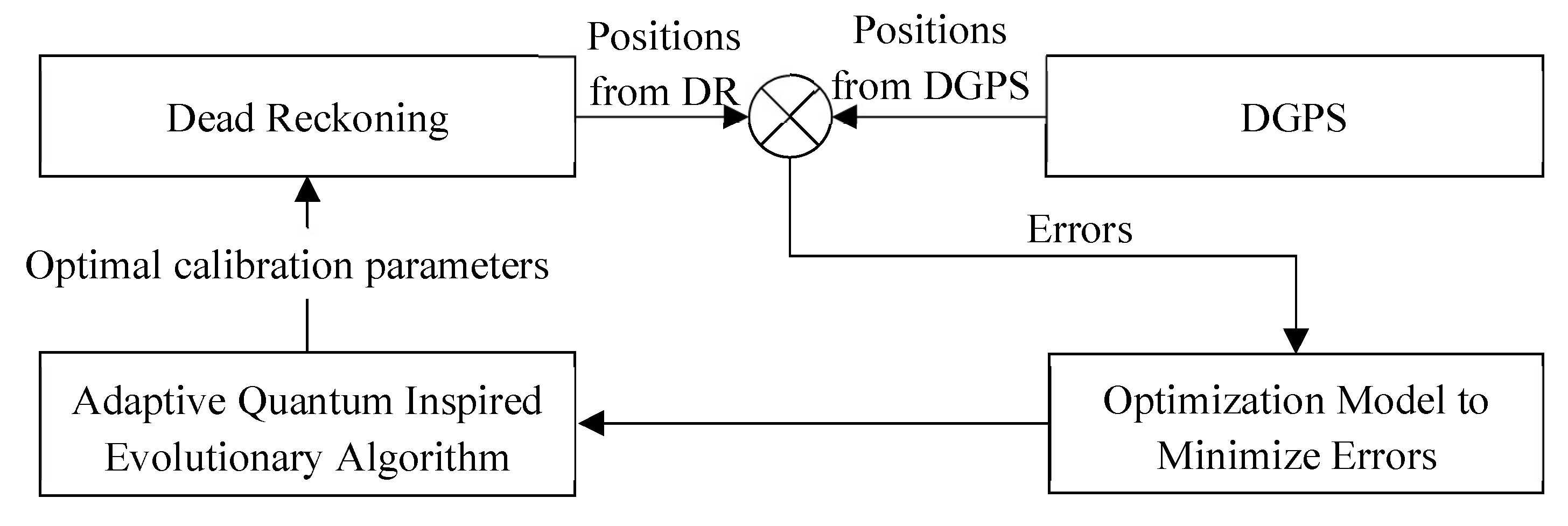
Figure 2 gives the process of parameter calibration based on the proposed dead reckoning calibration method. It should be noted that the differential GPS (DGPS) is only used for the calibration process and the initialization of DR localization.
To calibrate DR, the positioning data obtained from a high accuracy DGPS are used as the correct positions. The difference between the data from the DGPS and DR is considered as the positioning error, and it is calculated by
E i ( c 1 , c 2 , c 3 , p i G P S , p i D R ) = ( x i G P S x ˜ i ) 2 + ( y i G P S y ˜ i ) 2 i = 1 , 2 , , N
where Ei is the difference between the DR’s estimated position p i D R and the DGPS’s position p i G P S at the i-th time point, and N is the total number of sample points.
To identify the optimal calibration parameters of DR, an optimization model is formulated as:
min w . r . t . c 1 , c 2 , c 3 M s . t . c 1 L c 1 c 1 U c 2 L c 2 c 2 U c 3 L c 3 c 3 U
where c 1 L , c 1 U , c 2 L , c 2 U , c 3 L , and c 3 U are the lower and upper limits of c1, c2, and c3, respectively, and M is the optimization objective function related to positioning errors to be minimized. The ranges of c1, c2, and c3 are usually determined by real measurements; in this study, their ranges were set as [−1, 1], [−1, 1], and [−2, 2], respectively. To identify the optimal calibration parameters, two different optimization objective functions are tested. They are the maximum positioning error and the mean positioning error considering all the positioning data:
M = max w . r . t . i E i   or   M = 1 N i = 1 N E i

3. Optimization Based on an Adaptive Quantum-Inspired Evolutionary Algorithm

3.1. Process of the Adaptive Quantum-Inspired Evolutionary Algorithm

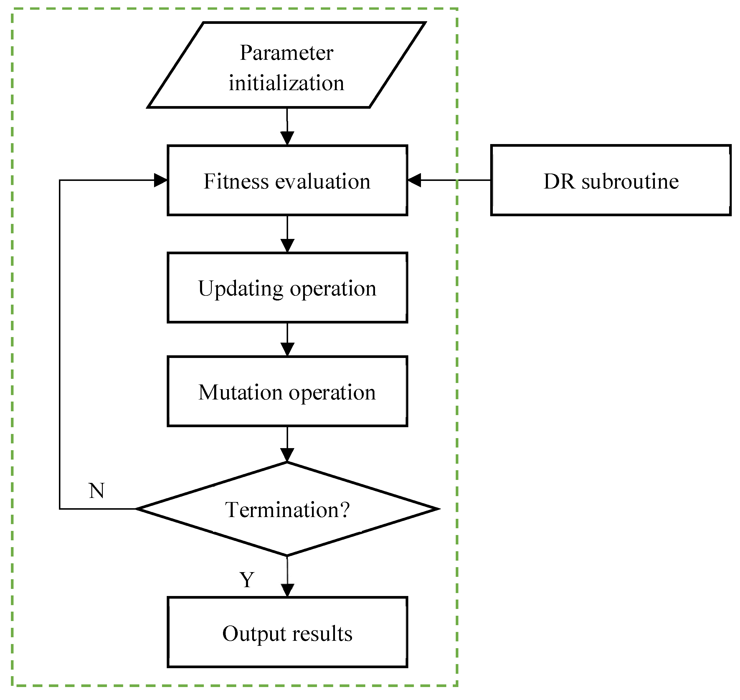
In this work, an adaptive quantum-inspired evolutionary algorithm (AQIEA) is introduced to solve the optimization problem defined in Equation (9). Figure 3 gives the flowchart of the AQIEA. In this algorithm, first a population of solutions is initialized. Each individual in this population is evaluated based on the fitness measure which is defined by the optimization objective function. In this work, a DR subroutine is used to calculate the optimization objective function evaluation measure. The individuals in the population are subsequently evolved using updating operations and mutation operations. When the optimization criteria are satisfied, the best individual in the population is selected as the optimal solution. Otherwise, the individuals need to be evolved again to generate better solutions.

3.2. Classic Quantum-Inspired Evolutionary Algorithm

The quantum-inspired evolutionary algorithm (QIEA) was introduced to improve optimization capabilities and has been employed to solve many different types of problems such as the 0–1 knapsack problem [23], stochastic job shop scheduling problem [24], neuro-fuzzy controller design problem [25], and function optimization problem [26].
QIEA was developed based on the principles and concepts in quantum computing, such as qubits and the superposition of states. In QIEA, qubit chromosomes, instead of binary, numeric, or symbolic chromosomes, are used to model optimization solutions. A qubit is the basic information unit in a two-state quantum computer. A qubit might be in the state 0 or state 1 , or in any linear superposition of the two states because of the advantage that a qubit can represent a linear superposition of state 0 and state 1 . Here, is the Dirac bracket notation.
A qubit is defined as:
| φ = α | 0 + β | 1
where | φ is a qubit state, and α and β are complex numbers to specify the probability amplitudes of the states 0 and 1 , respectively. |α|2 is the probability of outcome 0 , and |β|2 is the probability of outcome 1 . The α and β satisfy the following condition:
| α | 2 + | β | 2 = 1
If a system has m qubits, the system can present 2m states at the same time. However, in the act of observing the m qubits, the outcome is a single state. In the QIEA, an individual is composed of m qubits, and one qubit is defined by a pair of probability amplitudes α β . Thus, an individual with m qubits is defined by
q = α 1 β 1 α 2 β 2 α i β i α m β m
where q is an individual in the population, and α i 2 + β i 2 = 1 , i = 1, 2, …, m. The advantage of this representation is that an individual can represent any superposition of states. For example, an individual with three qubits can be represented as follows:
1 2 1 2 1 2 3 2 3 2 1 2
It can be used to represent eight different states in this system: 000 , 001 , 010 , 011 , 100 , 101 , 110 , and 111 , and probabilities of these states are calculated as: 3 32 , 1 32 , 9 32 , 3 32 , 3 32 , 1 32 , 9 32 , and 3 32 , respectively. After decoding the qubits to classic bits, the real values can be obtained by
x = x L + ( b 1 b 2 b 3 b n ) d e c i m a l 2 n 1 ( x U x L )
where x is the decoded real value, xU and xL are its lower and upper bounds, n is the length of the qubits for x, and (b1b2b3bn)decimal is decimal value of the classic bits (b1b2b3bn).
The evolution of QIEA is conducted through quantum operations on the qubits of individuals in the population. These quantum operations are usually called quantum gates. A quantum gate is a reversible gate represented by a unitary operator U acting on the qubit basis states. A unitary operator satisfies U+U = UU+, where U+ is the Hermitian adjoint of U. Although many quantum gates have been developed for quantum computing, only a quantum rotation gate is used in QIEA to update individuals during the evolution process. The quantum rotation gate UR(θ) is applied to update the probability amplitudes of quantum qubits in each individual to improve the quality of individuals in a population. U(θi) is defined by a matrix:
U R ( θ ) = cos ( θ ) sin ( θ ) sin ( θ ) cos ( θ )
where θ is the rotation angle.
For example, a qubit α i β i in an individual can be updated by a quantum rotation gate using
α i β i = U R ( θ i ) α i β i
where α i β i is the qubit after quantum rotation gate operation, and θi is the rotation angle determined by
θ i = s ( α i β i ) Δ θ i
where s(αiβi) is the sign of θi, and Δθi is the magnitude of the rotation angle. In the traditional QIEA, Δθi is selected based on experience and experiments. Different Δθi values for different cases are stored in a lookup table [23]. During the evolution process in QIEA, the lookup table is searched to identify the proper value for a specific qubit. Δθi is a key parameter in QIEA that influences computation quality and efficiency. When Δθi is too small, the algorithm may need too many iterations to converge into the optimal solution. When Δθi is too large, the solutions may be trapped into divergent locations or lead to a premature convergence to a local optimum.

3.3. The Adaptive Quantum-Inspired Evolutionary Algorithm

In this research, the classic quantum-inspired evolutionary algorithm (QIEA) has been modified to an adaptive quantum-inspired evolutionary algorithm (AQIEA) to improve optimization quality and efficiency.

3.3.1. Adaptive Population Updating Operation

In the classic QIEA, the population is primarily updated by the quantum rotation gate. The values of the rotation angles, however, are very difficult to select. Even though some rotation angles can be selected from the lookup tables, the values of these rotation angles are not changed during the population evolution process. Inspired by Xiong et al. [27], in this research, an adaptive QIEA (AQIEA) with a change of rotation angle in the evolution process is introduced to improve the quality and efficiency of the QIEA.
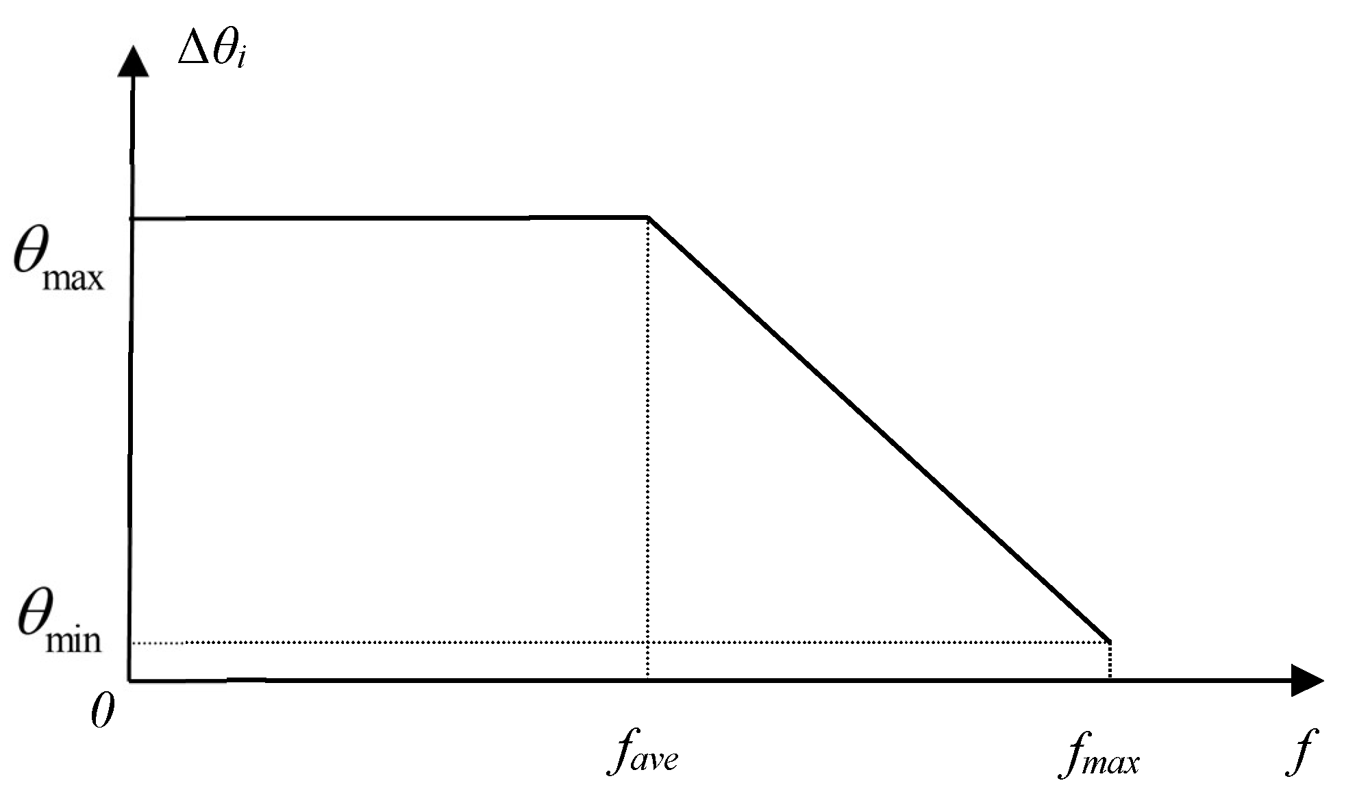
It has been found that when an individual is away from the optimal solution, a large value should be selected for the rotation angle to change the individual quickly towards the optimal solution. When an individual is close to the optimal solution, a small value should be selected for the rotation angle to avoid the individual moving away from the optimal solution. Based on this idea, an adaptive method is introduced in this research to adjust the value of the rotation angle in the optimization process. The magnitude of the rotation angle is calculated by
Δ θ i = θ max ( θ max θ min ) f f a v e f max f a v e f > f a v e θ max f f a v e
where θmax and θmin are two positive real numbers (0.001πθmin < θmax ≤ 0.5π). fmax is the maximum fitness in the current population, fave is the average fitness of the individuals in the current population, and f is the fitness of the selected individual. Figure 4 illustrates the adaptive change of the rotation angle magnitude of the quantum rotation gate. If the fitness of the selected individual is smaller than or equal to the average fitness of the current population, the magnitude of the rotation angle is selected as a constant θmax. If the fitness of the selected individual is larger than the average fitness of the current population, the magnitude of the rotation angle is then selected based on the value of f. When f = fmax, Δθi is selected as θmin.
The sign of the rotation angle is determined by
s ( α i β i ) = sgn ( ( o i * c ) α i β i ) α i β i 0 0 α i = 0   a n d   o i * = 1   o r   β i = 0   a n d   o i * = 0 ± 1 o t h e r
where sgn(•) is the sign function, oi* is the observed state (0 or 1) of the i-th qubit of the best individual, and c is a positive real number between 0 and 1. Equation (19) can be proved as follows.
Proof. 
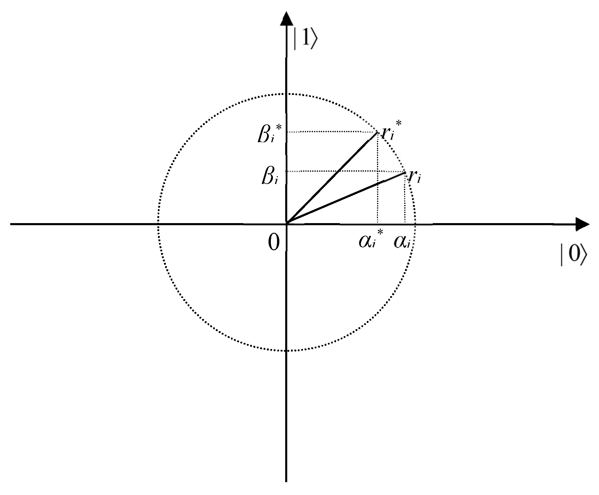
Assume ri* is the i-th qubit of the best individual, ri is the i-th qubit of the selected individual as shown in Figure 5 in the polar plot, and these qubits are represented as
r i * = α i * β i * , r i = α i β i
The observed states for the two states ri* and ri are defined by oi* and oi, respectively. □
The possible direction of the rotation angle is decided as follows:
(1) When oi* = 0 and oi = 1: if αiβi > 0, since ri lies in the I or III quadrant, s(αiβi) should be negative (i.e., −1) to increase the probability amplitudes of 0 ; if αiβi < 0, since ri lies in the II or IV quadrant, s(αiβi) should be positive (i.e., +1) to increase the probability amplitudes of 0 ; if αi = 0, since ri lies on the 1 axis, both +1 and −1 of s(αiβi) can increase the probability amplitudes of | 0 , so s(αiβi) is selected as ±1; if βi = 0, since ri lies on the 0 axis, the probability amplitudes of 0 are 1, so s(αiβi) is selected as 0.
(2) When oi* = 1 and oi = 0: if αiβi > 0, since ri lies in the I or III quadrant, s(αiβi) should be +1 to increase the probability amplitudes of 1 ; if αiβi < 0, since ri lies in the II or IV quadrant, s(αiβi) should be −1 to increase the probability amplitudes of 1 ; if αi = 0, since ri lies on the 1 axis, the probability amplitudes of | 1 are 1, so s(αiβi) is selected as 0; if βi = 0, since ri lies on the 0 axis, both +1 and −1 of s(αiβi) can increase the probability amplitudes of 0 , so s(αiβi) is selected as ±1.
(3) When oi* = 0 and oi = 0: if αiβi > 0, since ri lies in the I or III quadrant, s(αiβi) should be negative (i.e., −1) to increase the probability amplitudes of 0 ; if αiβi < 0, since ri lies in the II or IV quadrant, s(αiβi) should be positive (i.e., +1) to increase the probability amplitudes of 0 ; if αi = 0, since ri lies on the 1 axis, both +1 and −1 of s(αiβi) can increase the probability amplitudes of 0 , so s(αiβi) is selected as ±1; if βi = 0, since ri lies on the 0 axis, the probability amplitudes of 0 are 1, so s(αiβi) is selected as 0.
(4) When oi* = 1 and oi = 1: if αiβi > 0, since ri lies in the I or III quadrant, s(αiβi) should be +1 to increase the probability amplitudes of 1 ; if αiβi < 0, since ri lies in the II or IV quadrant, s(αiβi) should be −1 to increase the probability amplitudes of 1 ; if αi = 0, since ri lies on the 1 axis, the probability amplitudes of 1 are 1, so s(αiβi) is selected as 0; if βi = 0, since ri lies on the 0 axis, both +1 and −1 of s(αiβi) can increase the probability amplitudes of 0 , so s(αiβi) is selected as ±1.
Table 1 shows the summary based on the above discussions. It is found from Table 1 that the sign of the rotation angle is determined based on oi*, αi, and βi, but not oi. This is because when oi* = 1, the probability amplitudes of 1 should be increased, no matter if the value of oi is 0 or 1. Similarly, when oi* = 0, the probability amplitudes of 0 should be increased, no matter if the value of oi is 0 or 1.
The summary given in Table 1 can be simplified to the summary shown in Table 2. The sign in Equation (18) is obtained based on Table 2. For example, if αiβi > 0 and oi* = 0, the s(αiβi) is obtained as −1 according to Table 2.

3.3.2. Adaptive Mutation Operation

To avoid being trapped into local optimal locations and to improve global searching ability, an adaptive quantum mutation operation is introduced in this work in the AQIEA. For a selected individual in the population, the mutation operation is conducted based on a mutation probability:
p m = p max ( p max p min ) f f a v e f max f a v e i f   f > f a v e p max f f a v e
where pmax and pmin are two small positive real values between 0 and 1. When an individual is selected for mutation, two random positions in the individual are selected and the two qubits are mutated by a quantum-not gate. A quantum-not gate UX is defined by a matrix:
U X = 0 1 1 0
For example, a qubit α i β i in an individual can be mutated by a quantum-not gate through
α i β i = U X α i β i = β i α i
where α i β i is the qubit after quantum-not gate operation. Obviously, the quantum-not gate operation is used to swap the probability amplitudes of the two quantum states 0 and 1 .

3.3.3. The Procedures in AQIEA

With the proposed adaptive quantum rotation and mutation operations, the proposed quantum-inspired evolutionary algorithm can effectively enhance the population diversity and further accelerate the convergence speed and avoid being trapped in the local optimal. The detail procedures in AQIEA are described as follows (Procedure 1).
Procedure 1. Procedure of AQIEA.
Begin Proc
(1)
Set t = 0, initialize the population Q(t) by assigning each pair of αi and βi in each individual in Q(t) as 1 / 2 , representing that each qubit has the same probabilities to be observed as | 0 and | 1 at the initialization step;
(2)
Create a set of binary strings P(t) for representing the observing states of Q(t) based on the Procedure 2 (Procedure of decoding);
(3)
Evaluate all binary strings in P(t);
(4)
Store the best solution among all binary strings in P(t) as P*;
(5)
While (termination condition is not satisfied) do
(i)
Increase t’s value by t = t + 1;
(ii)
Create a set of binary strings P(t) for representing the observing states of Q(t) based on the Procedure 2;
(iii)
Evaluate all binary strings in P(t);
(iv)
Select the best solution among all binary strings in P(t), and compare it with the P*. If this best solution is better than P*, replace P* with this best solution; otherwise, keep P* unchanged;
(v)
Update individuals in Q(t) with the quantum rotation gate based on the Procedure 3 (Procedure of population updating);
(vi)
Apply mutation operation to individuals in Q(t) based on the Procedure 4 (Procedure of mutation operation).
  End while
End Proc
The decoding of a quantum individual into a classic bit individual is conducted based on the following Procedure 2.
Procedure 2. Procedure of decoding.
Begin Proc
For (each qj(t) in Q(t))
(1)
Initialize a binary string Pj(t) as a null list for representing the observing state of qj(t); initialize a decimal list Cj(t) as a null list for representing the selected values of parameters in optimization solution in the individual;
(2)
For (each pair of αi and βi in qj(t))
(i)
Generate a random number r between 0 and 1;
(ii)
If r ≥ |αi|2, the corresponding observing state of the qubit is 1; otherwise, the observing state is 0. Add the observing state to Pj(t).
  End for
(3)
Convert the binary string Pj(t) to a decimal list Cj(t) with values of parameters in an optimization solution based on Equation (15).
End for
End Proc
The adaptive population updating operation is conducted using the following Procedure 3.
Procedure 3. Procedure of population updating.
Begin Proc
For (each qj(t) in Q(t))
For (each pair of αi and βi in qj(t))
(i)
Calculate Δθi and s (αiβi) based on Equations (19) and (20), respectively;
(ii)
Update αi and βi based on Equations (16)–(18).
  End for
End for
End Proc
The adaptive mutation operation is conducted using the following Procedure 4.
Procedure 4. Procedure of mutation operation.
Begin Proc
For (each qj(t) in Q(t))
(1)
Generate a random number r between 0 and 1;
(2)
If r < pm, where pm is calculated from Equation (22), generate two random mutation positions p1 and p2 in qj(t). If p1p2, conduct mutation operations to the qubits in positions of p1 and p2 based on Equation (24); otherwise, do nothing;
(3)
Otherwise, do nothing.
End for
End Proc

4. Identification of the Optimal Calibration Parameters for Dead Reckoning Based on the AQIEA

4.1. Experimental Setup for Dead Reckoning

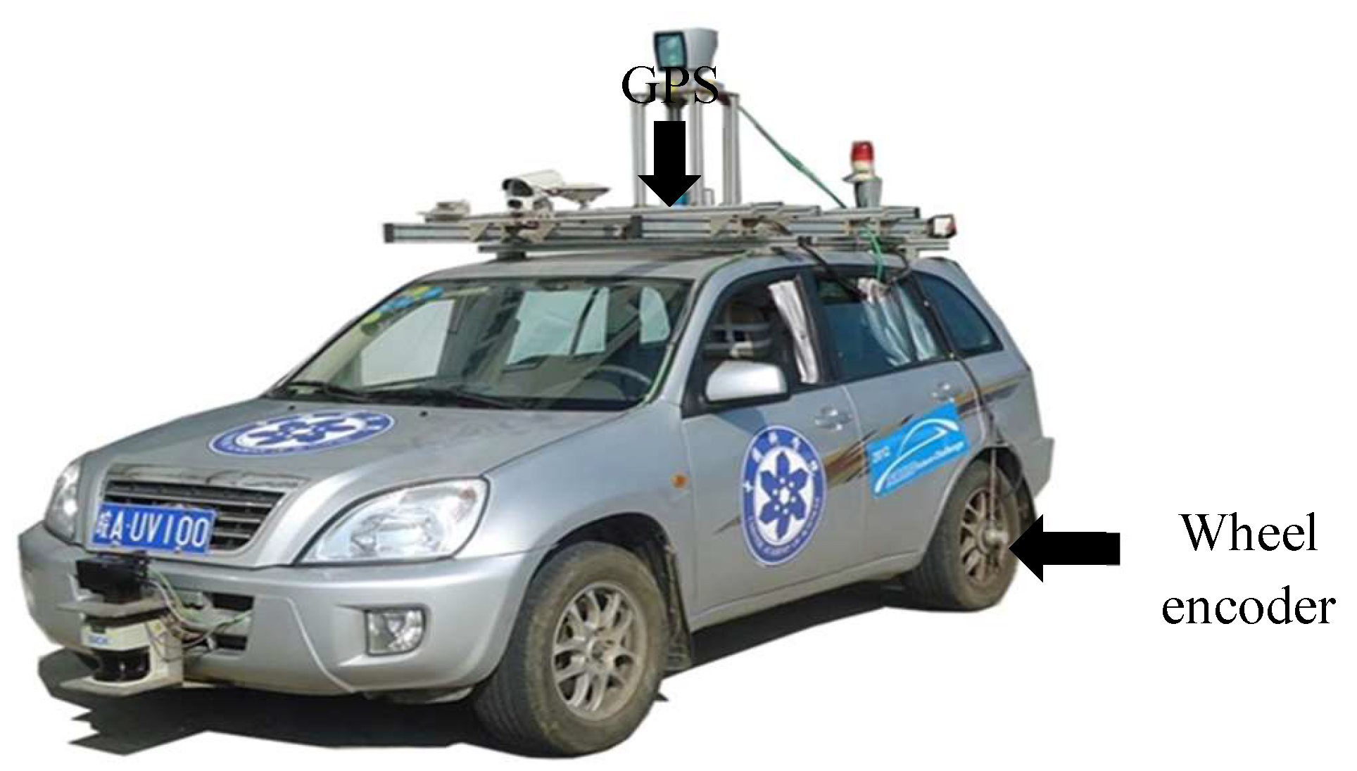
The intelligent vehicle experimental platform, “Intelligent Pioneer II” (Figure 6) developed by the Intelligent Vehicle Research Center, Hefei Institutes of Physical Science (HIPS), was used to carry out the dead reckoning experiments. Two wheel encoders that were mounted on the two rear wheels of the vehicle were used to provide the odometry readings, and the DGPS sensor (NovAtel SPAN-CPT), a tightly coupled GPS/INS integrated navigation system, was used to provide real-time positioning information for calculation of the localization errors and to initialize the dead reckoning system.
The nominal parameters of the vehicle and the sensors are given in Table 3.

4.2. Identification of the Optimal Dead Reckoning Calibration Parameters Based on the AQIEA

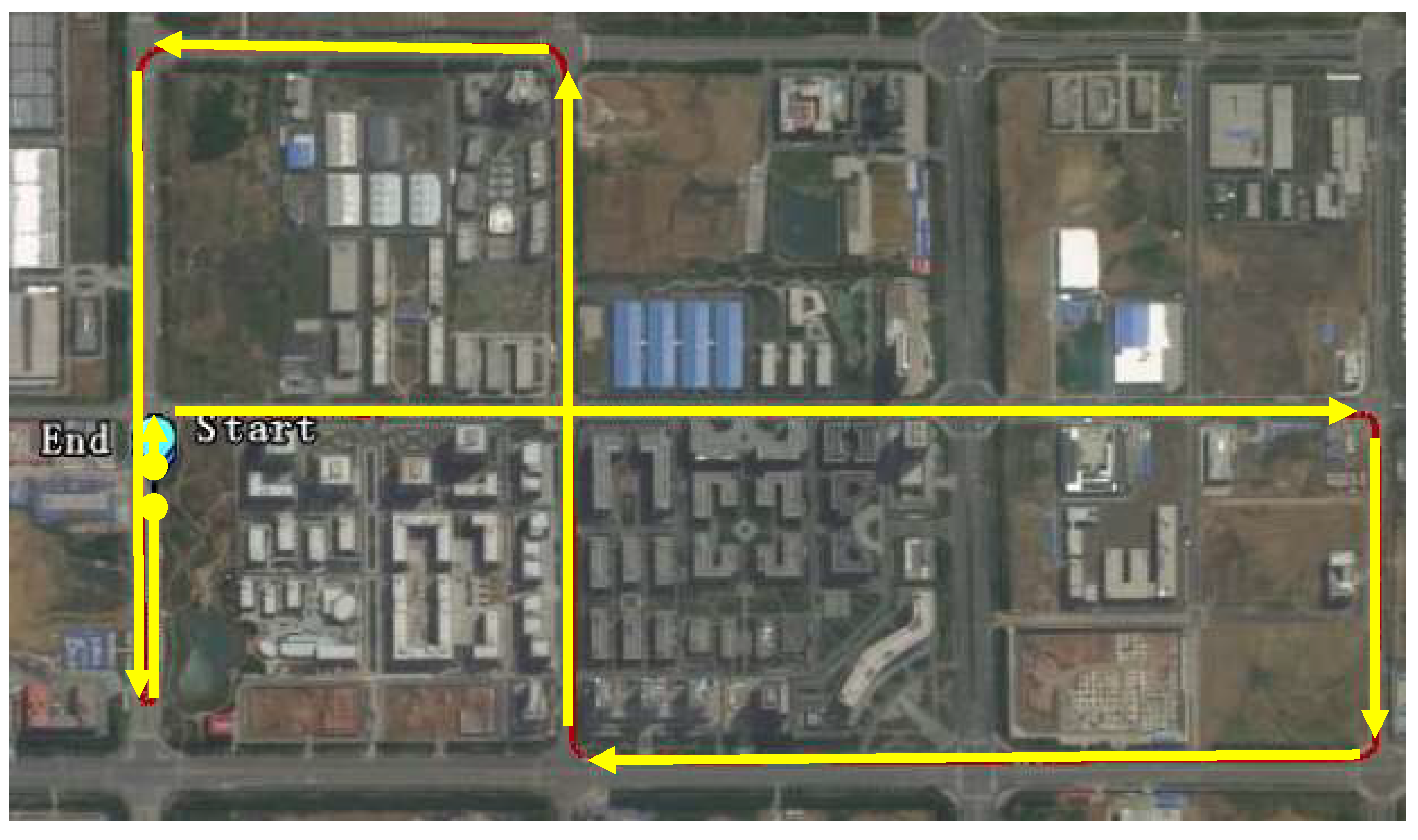
It should be noted that unlike traditional DR calibration methods such as UMBmark [4], the calibration path in this work was selected from normal suburb roads. Because the considered optimization parameters for the calibration are the compensation values to the left rear wheel, right rear wheel, and vehicle heading, the designed calibration path should contain enough scenarios (including both left and right turns) and enough mileage. To calibrate the DR, a calibration path needs to be selected as shown in Figure 7. The yellow arrows in the figure mean the driving directions and route. The total length of the calibration path was about 6 km.
During the experiment, the vehicle was driven along the selected path, and the positioning data (i.e., longitude, latitude, and heading) of the vehicle from the DGPS and the pulse readings from the two wheel encoders and the gyroscope were recorded simultaneously. Because the two different kinds of data from the DGPS and the DR were in different coordinate systems (i.e., DGPS in the WGS84 coordinate system and DR in the Cartesian coordinate system), these data had to be converted into the same coordinate system. In this work, the longitude and latitude from the DGPS were converted into the Cartesian coordinate system by
x t g p s = R cos ( φ t m ) Δ λ t y t g p s = R Δ φ t
where R = 6,371,004 m is the radius of the earth, ( x t g p s , y t g p s ) is the vehicle’s position at time t in the Cartesian coordinate system, and Δλt and Δφt are the differences of the longitude and latitude between the initial position and the position at time t, respectively. Δλt, Δφt, and φtm are defined by
Δ λ t = λ t λ 0 Δ φ t = φ t φ 0 φ t m = φ t + φ 0 2
where (λ0, φ0) and (λt, φt) are the initial position and the position at time t in the WGS84 coordinate system, respectively. The units of λ0, φ0, λt, and φt are radians.
After the data were collected, the maximum error and mean error considering all the positions were selected as the objective functions to build the two optimization models. For each optimization model, each of the three calibration parameters (i.e., c1, c2, and c3) was encoded by 20 qubits and so each individual was encoded by 60 qubits, the AQIEA was run 10 times, and the termination condition for the two optimization models was set as 10,000 generations.
For the first optimization model to minimize the maximum error, the optimal calibration parameters were obtained as: c1 = 0.642 m, c2 = −0.455 m, and c3 = 0.377°. The maximum positioning error was obtained as 4.7398 m. For the second optimization model to minimize the mean error, the optimal calibration parameters were obtained as: c1 = 0.177 m, c2 = 0.020 m, and c3 = 0.425°. The mean positioning error was obtained as 1.6838 m.
Figure 8 (the y-axes are plotted with logarithmic scale) gives the errors along the selected calibration path for the three different DR positioning datasets, i.e., DR without parameter calibration, DR with parameter calibration through minimization of the maximum error, and DR with parameter calibration through minimization of the mean error. From the figure, it is can be found that, compared to the result of DR without parameter calibration, the DR with the parameter calibration through two different optimization models can improve the positioning accuracy significantly. From the figure, it can also be seen that the DR data with the parameter calibration through minimization of the mean error can provide the best results. Thus, the calibration parameters obtained through minimization of the mean error were selected as the final calibration parameters.

4.3. Experiments for Dead Reckoning with Error Compensation

Two different dead reckoning experiments with different scales of the road paths were conducted to evaluate the effectiveness of the developed calibration scheme. The first road path was about 16 km, and the second one was about 43 km. In these two experiments, the same calibration parameters that were obtained as explained in Section 4.2 were used in the dead reckoning model, and the DGPS was just used for obtaining the headings of the vehicle and the error calculations. The DR self-localization was conducted in real time during the driving processes.
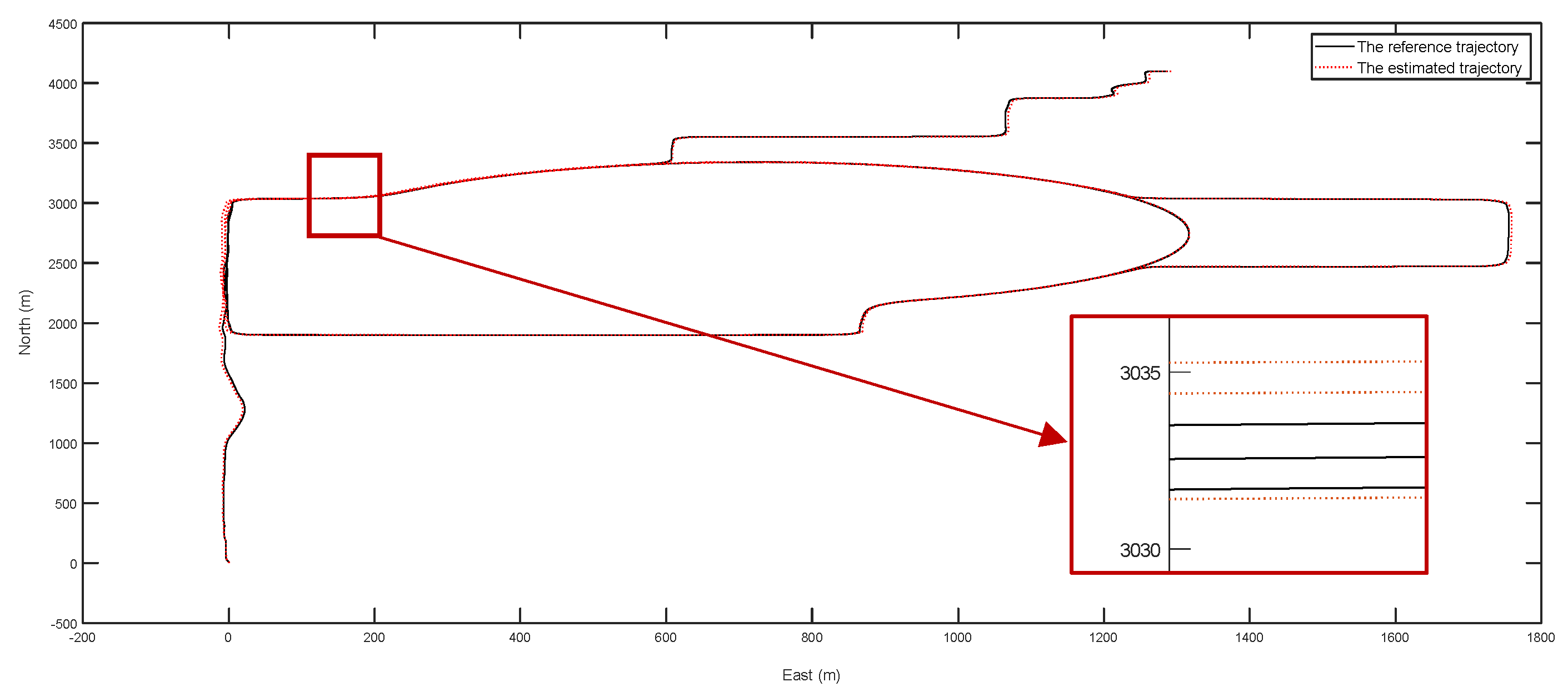
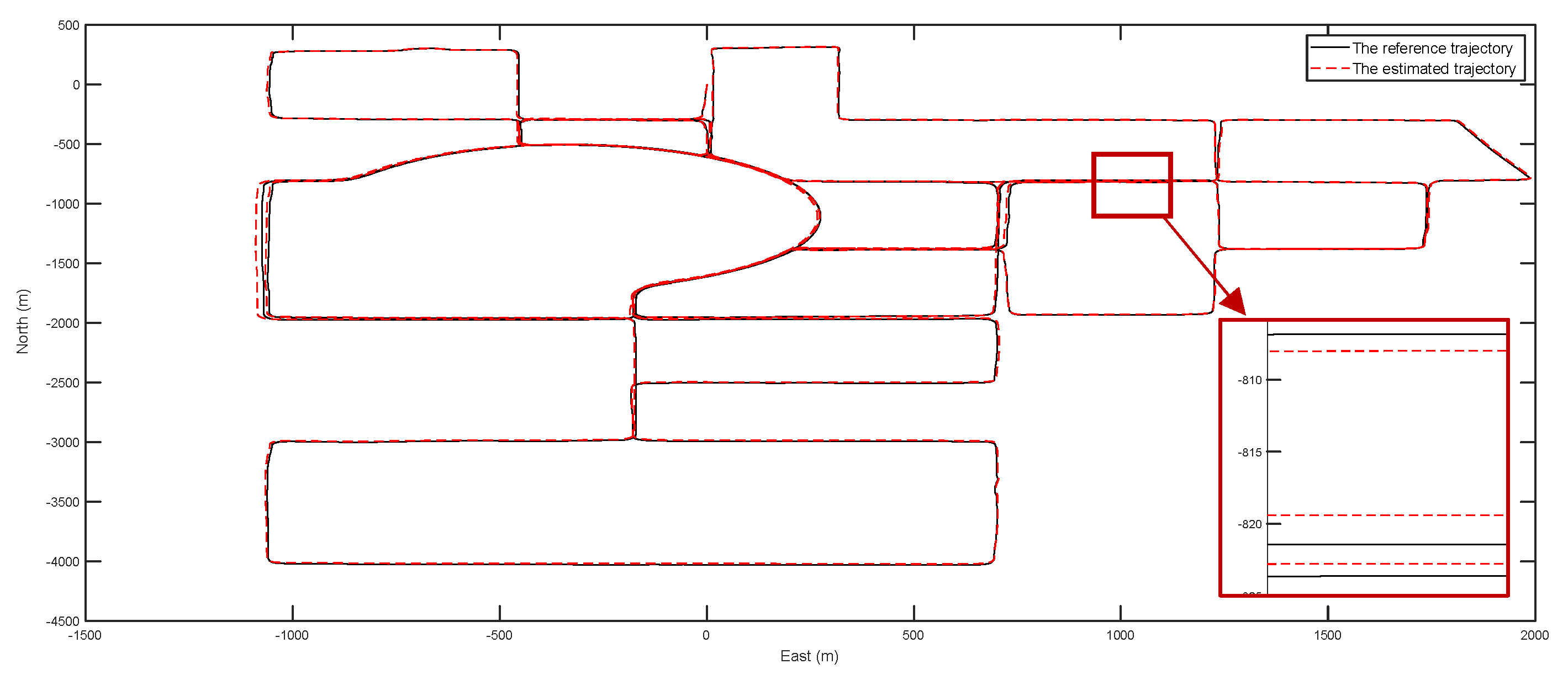
The reference trajectory (DGPS) and estimated trajectory for the two tests are given in Figure 9 and Figure 10, respectively. During the two experiments, some road segments were repeated twice to test the repeatability of the positioning accuracy (which is similar to the closure error) of the calibrated dead reckoning-based positioning method. From the experimental results, it was found that the maximum repeated error of positioning accuracy was about 1 m for the 16 km test and 3 m for the 43 km test.
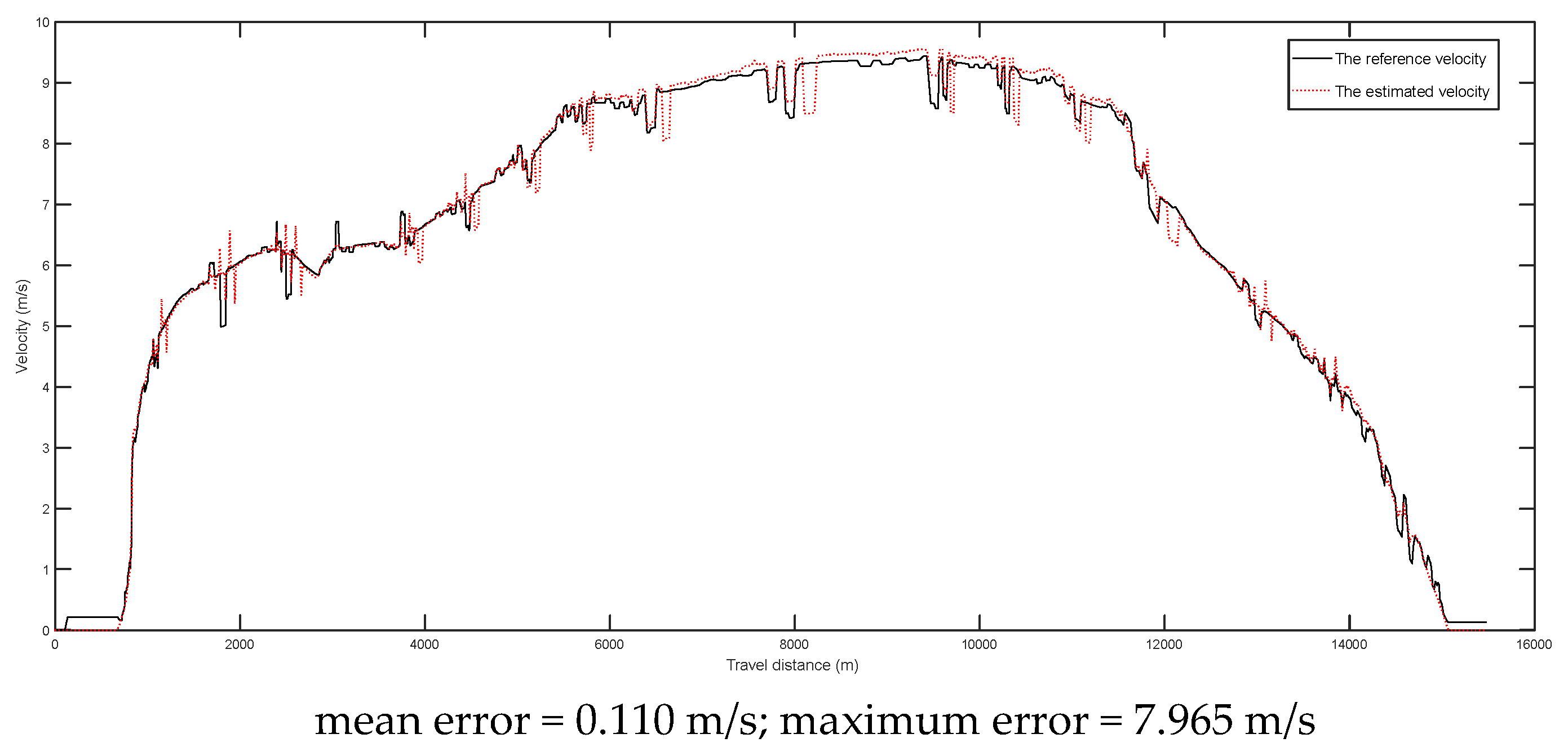
The comparison between the reference velocities (DGPS) and the estimated velocities during the two tests are given in Figure 11 and Figure 12, respectively. From the results, it was found that the mean velocity errors were reduced to 0.110 m/s and 0.070 m/s for the tests of 16 km and 43 km, respectively. It should be noted that the large maximum errors were due to the random noises.
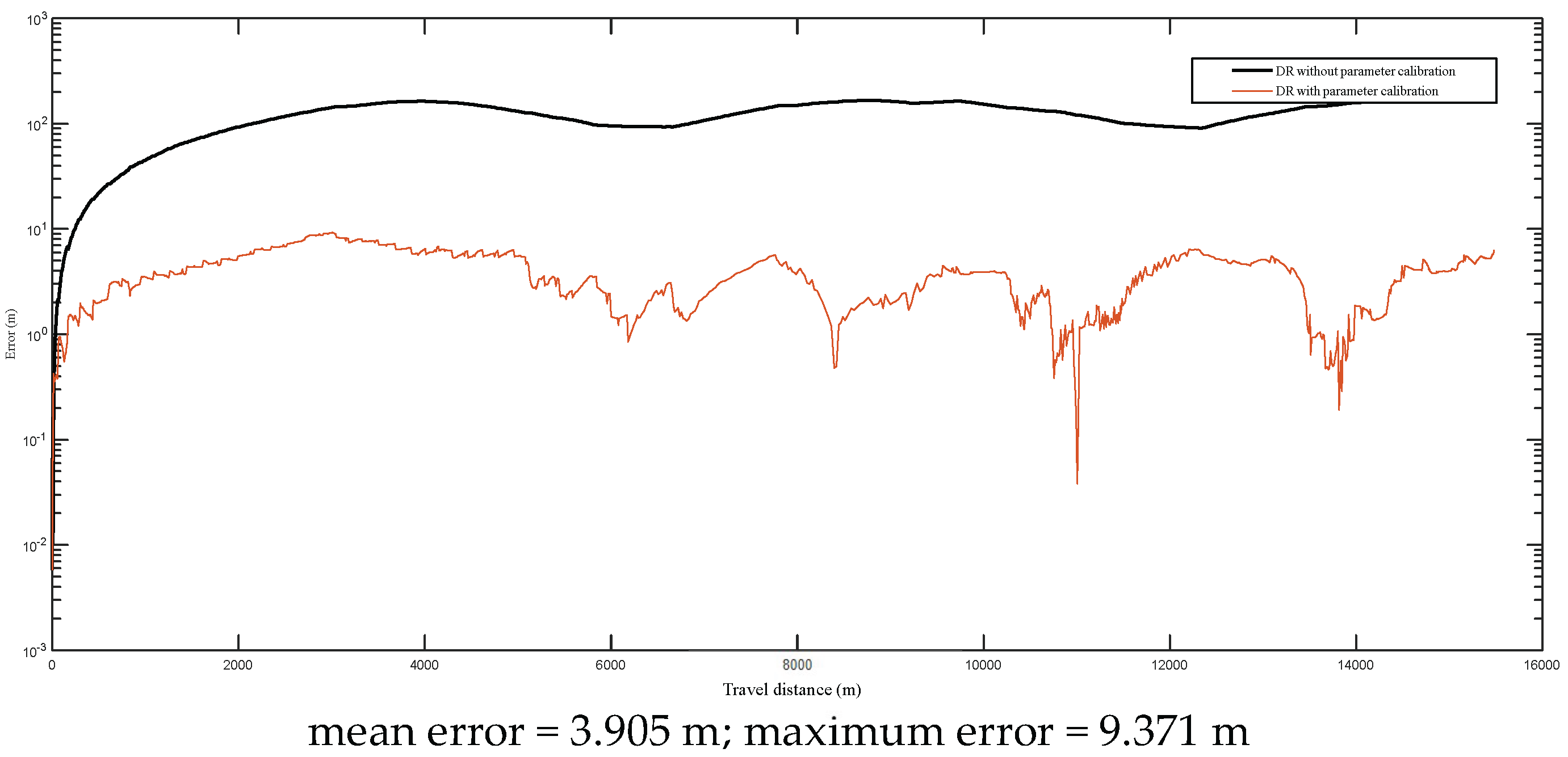
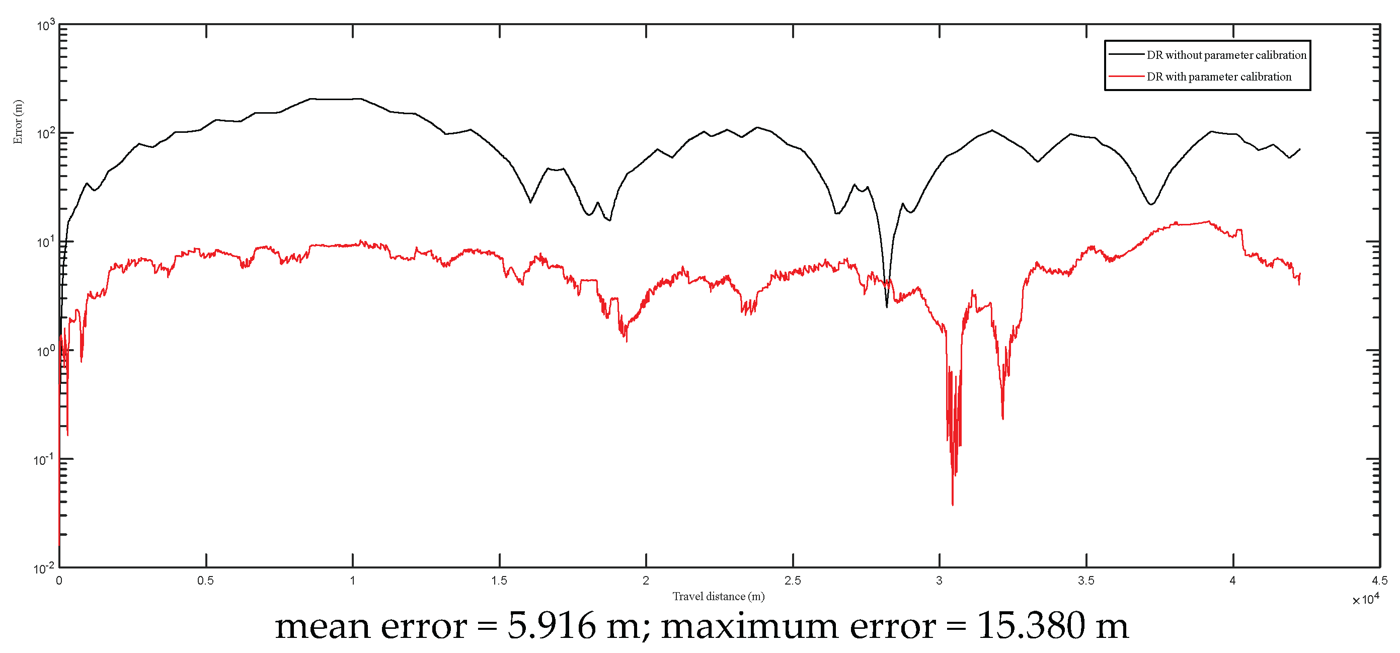
The positional errors are given in Figure 13 and Figure 14 (the y-axes are plotted with logarithmic scale), respectively. From the experimental results, it can be found that the maximum errors reached up to 200 m during the 16 km and 42 km field tests. After the calibrated parameters were applied, the maximum and mean errors were reduced significantly. For the 16 km test, its mean error and maximum error were reduced to 3.905 m and 9.371 m, respectively. For the 42 km test, its mean error and maximum error were reduced to 5.916 m and 15.380 m, respectively. It should be noted that the curve shapes of DR errors follow different patterns due to the change of the vehicle’s driving direction. When the driving direction is not changed, the DR errors may be increased continuously. When the driving direction is changed or driving on driving on a trajectory where there are loop routes, such as the selected test trajectories in this study (e.g., Figure 7, Figure 9 and Figure 10), the DR errors can be reduced. The detailed analysis can be consulted in reference [4].
From the above experimental results, it can be concluded that the developed method can be used to calibrate the dead reckoning parameters to reduce the systematic errors effectively. With this method, the dead reckoning can be used as an alternative high accuracy localization tool when the GPS is out of service.

5. Comparative Study for the AQIEA

5.1. Benchmark Functions

To further demonstrate the quality and efficiency of the newly developed AQIEA optimization method, the AQIEA was compared with the classic genetic algorithm (CGA) [28] and the classic quantum-inspired evolutionary algorithm (CQIEA) [23]. Eight benchmark functions were selected to evaluate the performance of these three algorithms. The search spaces of the first four functions (f1~f4) are 2-dimensional and the search spaces of the other four functions (f5~f8) are 30-dimensional. Table 4 gives the detailed descriptions of the eight benchmark functions. In this table, D is the dimension of the search space, R is the value range of each variable, and O is the optimal value under the given constraints.

5.2. Results for Comparative Study

To test these benchmark functions, the specific parameters for the three algorithms must be given. Table 5 provides parameter settings for these three algorithms. It should be noted that to keep the manuscript more concise, the quantum rotation angles in CQIEA were omitted and can be consulted in reference [23]. Because the complexities of the eight functions are different, different maximum iterations were selected to obtain the best results. In this comparative study, the maximum generations were selected as 5000 for functions f1~f4, and the maximum generations were selected as 10,000 for functions f5~f8.
All the three algorithms were implemented in MATLAB running on a computer with the Intel Core i3-3129M (dual cores 2.4G) CPU and the RAM of 2 GB. Due to the stochastic nature of the evolutionary algorithm, each algorithm was run 30 times for each benchmark function. Table 6 gives the experimental results of the three algorithms. In this table, the best value, the worst value, the mean value, the standard deviation, and the mean computation time considering the 30 runs for each of the test function using each of the evolutionary algorithms are provided.
From Table 6, we can see that the adaptive quantum-inspired evolutionary algorithm (AQIEA) developed in this research nearly provides the best computation quality and efficiency among the selected three algorithms. The AQIEA takes the shortest time because it needs a smaller population size than CGA to achieve the optimization results, and unlike CQIEA, it does not need to search the lookup table for conducting the quantum rotation operations.
From the experimental results, it can be found that by applying the adaptive quantum rotation operation and the adaptive quantum mutation operation, the developed AQIEA can effectively prevent the optimization results from being trapped into divergent locations or premature convergence to local optimums. Due to the search ability of the proposed algorithm, it is very effective at optimizing the error function for dead reckoning to obtain optimal calibration parameters.

6. Conclusions

The developed method aims at reducing systematic errors of dead reckoning-based positioning for intelligent vehicles. In this study, an adaptive quantum-inspired evolutionary algorithm-based dead reckoning calibration scheme was proposed. Real road experiments were conducted to evaluate the effectiveness of the developed method and the experiment results show that the maximum error and average error of dead reckoning can be reduced significantly. With this method, the dead reckoning can be used as an alternative high accuracy localization tool when the GPS is out of service. Advantages of the developed method are summarized as follows:
(1)
The newly developed dead reckoning positioning parameter calibration scheme is effective at compensating the systematic errors in dead reckoning. In addition, the design of a special calibration path is not required in this method for the calibration experiment.
(2)
The developed adaptive quantum-inspired evolutionary algorithm is effective at identifying the optimal calibration parameters for the dead reckoning.
(3)
The adaptive quantum rotation operation and the adaptive quantum mutation operation introduced in this research are effective at improving the computation quality and efficiency of the quantum-inspired evolutionary algorithm.
The developed calibration method was only tested on paved road with a smooth surface and only systematic errors of dead reckoning were considered. Additional tests will be conducted on different road conditions and an improved method which considers both systematic errors and random errors will be developed in the future. Moreover, for the proposed adaptive quantum-inspired evolutionary algorithm, a multi-objective version will be developed in the future.

Author Contributions

Conceptualization, B.Y. and B.L.; methodology, H.Z.; software, B.Y.; validation, L.X. and S.Z.; formal analysis, B.Y.; investigation, B.Y.; resources, B.Y.; data curation, B.L.; writing—original draft preparation, B.Y.; writing—review and editing, D.X.; visualization, B.L.; supervision, B.L.; project administration, B.Y.; funding acquisition, B.Y. All authors have read and agreed to the published version of the manuscript.

Funding

This work was partially supported by the Youth Innovation Promotion Association of the Chinese Academy of Sciences (Grant No. Y2021115).

Institutional Review Board Statement

Not applicable.

Informed Consent Statement

Not applicable.

Data Availability Statement

Not applicable.

Conflicts of Interest

The authors declare no conflict of interest.

References

  1. Quddus, M.A.; Noland, R.B.; Ochieng, W.Y. The effects of navigation sensors and spatial road network data quality on the performance of map matching algorithms. Geoinformatica 2009, 13, 85–108. [Google Scholar] [CrossRef]
  2. Borenstein, J.; Everett, H.R.; Feng, L.; Wehe, D. Mobile robot positioning: Sensors and techniques. J. Robot. Syst. 1997, 14, 231–249. [Google Scholar] [CrossRef]
  3. Zhao, L.; Ochieng, W.Y.; Quddus, M.A.; Noland, R.B. An extended Kalman filter algorithm for integrating GPS and low cost dead reckoning system data for vehicle performance and emissions monitoring. J. Navig. 2003, 56, 257–275. [Google Scholar] [CrossRef]
  4. Borenstein, J.; Feng, L. Measurement and correction of systematic odometry errors in mobile robots. IEEE Trans. Robot. Autom. 1996, 12, 869–880. [Google Scholar] [CrossRef]
  5. Cho, B.S.; Moon, W.S.; Seo, W.J.; Baek, K.W. A dead reckoning localization system for mobile robots using inertial sensors and wheel revolution encoding. J. Mech. Sci. Technol. 2011, 25, 2907–2917. [Google Scholar] [CrossRef]
  6. Zhang, J.; Singh, S. Low-drift and real-time lidar odometry and mapping. Auton. Robot. 2017, 41, 401–416. [Google Scholar] [CrossRef]
  7. Takeyama, K.; Machida, T.; Kojima, Y.; Kubo, N. Improvement of Dead Reckoning in Urban Areas Through Integration of Low-Cost Multisensors. IEEE Trans. Intell. Veh. 2017, 2, 278–287. [Google Scholar] [CrossRef]
  8. Bento, L.C.; Nunes, U.; Moita, F.; Surrécio, A. Sensor fusion for precise autonomous vehicle navigation in outdoor semi-structured environments. In Proceedings of the IEEE Intelligent Conference on Intelligent Transportation Systems, Vienna, Austria, 16 September 2005. [Google Scholar]
  9. Surrécio, A.; Nunes, U.; Araújo, R. Fusion of odometry with magnetic sensors using Kalman filters and augmented system models for mobile robot navigation. In Proceedings of the IEEE International Symposium on Industrial Electronics, Dubrovnik, Croatia, 20–23 June 2005. [Google Scholar]
  10. Philippe, B.; Pascal, B. Data fusion of four ABS sensors and GPS for an enhanced localization of car-like vehicles. In Proceedings of the IEEE International Conference on Robotics and Automation, Seoul, Korea, 21–26 May 2001. [Google Scholar]
  11. Lee, H.; Jung, J.; Choi, K.; Park, J.; Myung, H. Fuzzy-logic-assisted interacting multiple model (FLAIMM) for mobile robot localization. Robot. Auton. Syst. 2012, 60, 1592–1606. [Google Scholar] [CrossRef]
  12. Antonelli, G.; Chiaverini, S.; Fusco, G. A calibration method for odometry of mobile robots based on the least-squares technique: Theory and experimental validation. IEEE Trans. Robot. 2005, 21, 994–1004. [Google Scholar] [CrossRef]
  13. Lee, K.; Jung, C.; Chung, W. Accurate calibration of kinematic parameters for two wheel differential mobile robots. J. Mech. Sci. Technol. 2011, 25, 1603–1611. [Google Scholar] [CrossRef]
  14. Lee, K.; Chung, W.; Yoo, K. Kinematic parameter calibration of a car-like mobile robot to improve odometry accuracy. Mechatronics 2010, 20, 582–595. [Google Scholar] [CrossRef]
  15. Dogruer, C.U. Estimation of odometer parameters with MMAE and LSE. In Proceedings of the IEEE/ASME International Conference on Advanced Intelligent Mechatronics, Besacon, France, 8–11 July 2014. [Google Scholar]
  16. Philip, J.M.; Danny, R. Calibrating a 4-wheel mobile robot. In Proceedings of the IEEE/RSJ International Conference on Intelligent Robots and Systems, Lausanne, Switzerland, 30 September–5 October 2002; Volume 1, pp. 859–864. [Google Scholar]
  17. Paulo, A.J.; Bijan, S. Laser interferometry measurements based calibration and error propagation identification for pose estimation in mobile robots. Robotica 2014, 32, 165–174. [Google Scholar]
  18. Martinelli, A. The odometry error of a mobile robot with a synchronous drive system. IEEE Trans. Robot. Autom. 2002, 18, 399–405. [Google Scholar] [CrossRef]
  19. Lundquist, C.; Karlsson, R.; Özkan, E. Tire radii estimation using a marginalized particle filter. IEEE Trans. Intell. Transp. Syst. 2014, 15, 663–672. [Google Scholar] [CrossRef]
  20. Li, F.; Bonnifait, P.; Ibanez-Guzman, J. Map-aided dead-reckoning with lane-level maps and integrity monitoring. IEEE Trans. Intell. Veh. 2018, 3, 81–91. [Google Scholar] [CrossRef]
  21. Belhajem, I.; Maissa, Y.B.; Tamtaoui, A. Improving low cost sensor based vehicle positioning with Machine Learning. Control Eng. Pract. 2018, 74, 168–176. [Google Scholar] [CrossRef]
  22. Yu, B.; Dong, L.; Xue, D.; Zhu, H.; Geng, X.; Huang, R.; Wang, J. A hybrid dead reckoning error correction scheme based on extended Kalman filter and map matching for vehicle self-localization. J. Intell. Transp. Syst. Technol. Plan. Oper. 2019, 23, 84–98. [Google Scholar] [CrossRef]
  23. Han, K.H.; Kim, J.H. Genetic quantum algorithm and its application to combinatorial optimization problem. In Proceedings of the 2000 Congress on Evolutionary Computation, La Jolla, CA, USA, 16–19 July 2000. [Google Scholar]
  24. Gu, J.W.; Gu, X.S.; Gu, M.Z. A novel parallel quantum genetic algorithm for stochastic job shop scheduling. J. Math. Anal. Appl. 2009, 355, 63–81. [Google Scholar] [CrossRef]
  25. Li, P.C.; Song, K.P.; Shang, F.H. Double chains quantum genetic algorithm with application to neuro-fuzzy controller design. Adv. Eng. Softw. 2011, 42, 875–886. [Google Scholar] [CrossRef]
  26. Li, P.C. A quantum-behaved evolutionary algorithm based on the Bloch spherical search. Commun. Nonlinear Sci. Numer. Simul. 2014, 19, 763–771. [Google Scholar] [CrossRef]
  27. Xiong, H.; Wu, Z.; Fan, H.; Li, G.; Jiang, G. Quantum rotation gate in quantum-inspired evolutionary algorithm: A review, analysis and comparison study. Swarm Evol. Comput. 2018, 42, 43–57. [Google Scholar] [CrossRef]
  28. Chipperfield, A.J.; Fleming, P.J. The MATLAB genetic algorithm toolbox. In Proceedings of the IEEE Colloquium on Applied Control Techniques Using Matlab, London, UK, 26 January 1995. [Google Scholar]
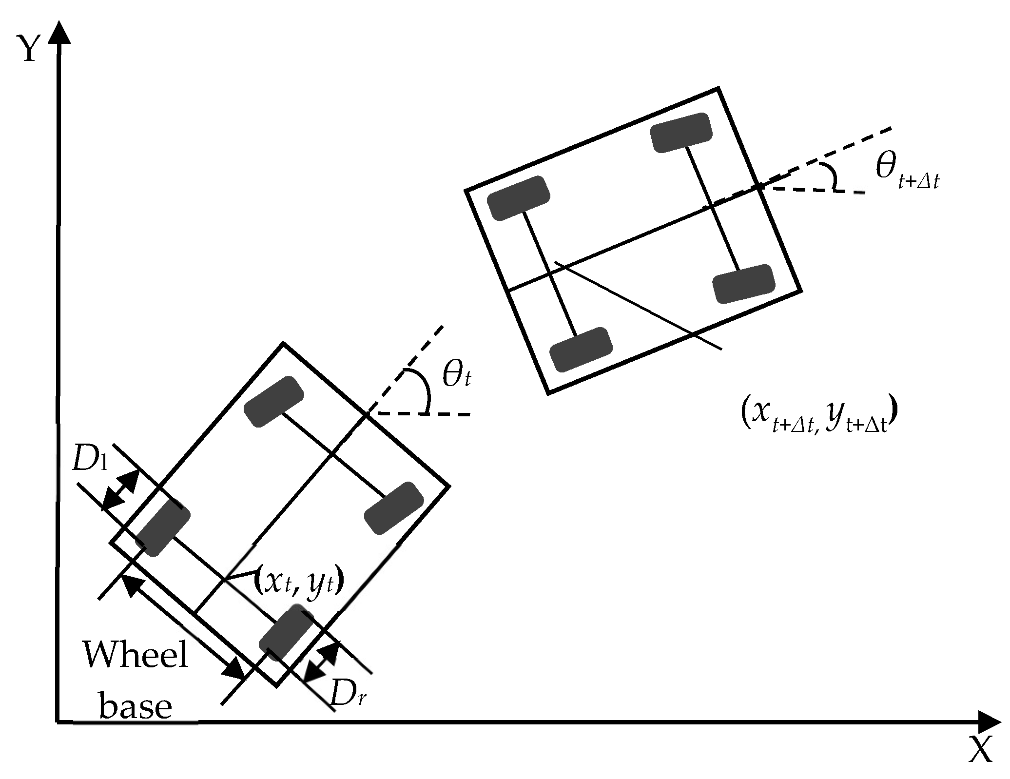
Figure 1. The dead reckoning localization process.
Entropy 24 01128 g001
Figure 2. Optimization-based dead reckoning calibration scheme.
Entropy 24 01128 g002
Figure 3. Optimization process based on AQIEA.
Entropy 24 01128 g003
Figure 4. Adaptive change of rotation angle magnitude of quantum rotation gate.
Entropy 24 01128 g004
Figure 5. Polar plot of quantum rotation gate for qubit.
Entropy 24 01128 g005
Figure 6. “Intelligent Pioneer II” intelligent vehicle experimental platform.
Entropy 24 01128 g006
Figure 7. The selected calibration path.
Entropy 24 01128 g007
Figure 8. Errors along the test path for the three different DR localization methods.
Entropy 24 01128 g008
Figure 9. The reference trajectory and estimated trajectory of the first test (about 16 km).
Entropy 24 01128 g009
Figure 10. The reference trajectory and estimated trajectory of the second test (about 43 km).
Entropy 24 01128 g010
Figure 11. The comparison between reference velocities and estimated velocities during the first test (about 16 km).
Entropy 24 01128 g011
Figure 12. The comparison between reference velocities and estimated velocities during the second test (about 42 km).
Entropy 24 01128 g012
Figure 13. The positional errors of the first test (about 16 km).
Entropy 24 01128 g013
Figure 14. The positional errors of the second test (about 43 km).
Entropy 24 01128 g014
Table 1. Summary of signs for the rotation angle.
oioi*s(αiβi)
αiβi > 0αiβi < 0αi = 0βi = 0
10−1+1±10
01+1−10±1
00−1+1±10
11+1−10±1
Table 2. Simplified summary of signs for the rotation angle.
oi*s(αiβi)
αiβi > 0αiβi < 0αi = 0βi = 0
0−1+1±10
1+1−10±1
Table 3. The nominal parameters of the vehicle and the sensors.
ParameterNameValue
RrResolution of encoder for rear right wheel 4000 pulses/r
RlResolution of encoder for rear left wheel4000 pulses/r
DrNominal diameter of right rear wheel0.637 m
DlNominal diameter of left rear wheel0.637 m
Table 4. Benchmark test functions.
No.FunctionFormulationDRO
f1De-Jong’s function f 1 = 100 ( x 1 2 x 2 ) 2 + ( 1 x 1 ) 2 2[−2.048, 2.048]0
f2Goldstein–Price function f 2 = [ 1 + ( x 1 + x 2 + 1 ) 2 ( 19 14 x 1 +    3 x 2 2 14 x 2 + 6 x 1 x 2 ) + 3 x 2 2 ]    [ 30 + ( 2 x 1 3 x 2 ) 2 ( 18 32 x 1 +    12 x 1 2 + 48 x 2 36 x 1 x 2 + 27 x 2 2 ) ] 2[−100, 100]3
f3Schaffer’s F6 function f 3 = 0.5 + sin 2 x 1 2 + x 2 2 0.5 [ 1 + 0.001 ( x 1 2 + x 2 2 ) ] 2 2[−100, 100]0
f4Easom’s function f 4 = cos ( x 1 ) cos ( x 2 )    exp [ ( x 1 π ) 2 ( x 2 π ) 2 ] 2[−100, 100]−1
f5Sphere function f 5 = i = 1 n x i 2 30[−5.12, 5.12]0
f6Griewank function f 6 = 1 4000 i = 1 n x i 2 i = 1 n cos ( x i i ) + 1 30[−600, 600]0
f7Ackley function f 7 = 20 exp ( 0.2 1 n i = 1 n x i 2 ) -    exp [ 1 n i = 1 n cos ( 2 π x i ) ] + 20 + e 30[−32, 32]0
f8Rastrigin function f 8 = i = 1 n x i 2 10 cos ( 2 π x i ) + 10 30[−5.12, 5.12]0
Table 5. Main parameters for comparing the three algorithms.
ParameterCGACQIEAAQIEA
Population size601010
Maximum generation5000 for f1~f4
10,000 for f5~f8
5000 for f1~f4
10,000 for f5~f8
5000 for f1~f4
10,000 for f5~f8
Crossover rate0.7//
Mutation rate0.01/pmax = 0.1,
pmin = 0.01
Quantum rotation angle/Given in [23]θmax = 0.05π,
θmin = 0.001π
Table 6. Experimental results of the three algorithms.
Test FunctionPerformanceAlgorithms
AQIEACGACQIEA
f1Best value1.0004 × 10−101.0004 × 10−108.2224 × 10⁻⁸
Worst value8.0830 × 10−21.9749 × 10−11.0000
Mean value7.3313 × 10−35.0742 × 10−27.9007 × 10−2
Standard deviation1.7405 × 10−26.4377 × 10−22.5115 × 10−1
Mean time (s)15.830.225.3
f2Best value3.00003.00003.0000
Worst value8.4600 × 1015.7482 × 1056.1677 × 107
Mean value9.04481.9191 × 1042.0560 × 106
Standard deviation1.6197 × 1011.0494 × 1051.1261 × 107
Mean time (s)13.930.428.8
f3Best value1.8190 × 10−81.8190 × 10−81.8190 × 10−8
Worst value9.6583 × 10−31.2439 × 10−11.2439 × 10−1
Mean value5.9255 × 10−31.4411 × 10−21.0522 × 10−2
Standard deviation4.5687 × 10−33.0204 × 10−22.1957 × 10−2
Mean time (s)19.957.225.8
f4Best value−1.0000−1.0000−1.0000
Worst value−1.0000−4.6552 × 10−70.0000
Mean value−1.0000−9.6631 × 10⁻¹−3.3333 × 10⁻²
Standard deviation0.00001.8251 × 10−11.8257 × 10⁻¹
Mean time (s)13.630.028.9
f5Best value1.6051 × 10−54.16211.2827 × 10−4
Worst value2.5806 × 10−27.38582.1318 × 10−1
Mean value1.3603 × 10−35.82917.9335 × 10−3
Standard deviation4.6669 × 10−38.3242 × 10−13.8769 × 10−2
Mean time (s)277.2374.4637.2
f6Best value6.2675 × 10−51.6512 × 1011.9451 × 102
Worst value1.8752 × 10−52.6707 × 1019.4725 × 101
Mean value4.6470 × 10−52.2313 × 1013.4142 × 101
Standard deviation4.5904 × 10−52.33072.1200 × 101
Mean time (s)270.5382.6614.7
f7Best value3.3597 × 10−19.05549.99160
Worst value4.32681.0766 × 1011.9265 × 101
Mean value2.11131.0020 × 1011.3341 × 101
Standard deviation7.8542 × 10−14.2962 × 10−12.5355
Mean time (s)347.7373.9657.9
f8Best value8.19574.0974 × 1016.6567 × 101
Worst value2.4041 × 1018.5433 × 1018.7187 × 101
Mean value1.3444 × 1016.2210 × 1017.9928 × 101
Standard deviation3.99401.1466 × 1015.1744
Mean time (s)328.6356.7643.1
Publisher’s Note: MDPI stays neutral with regard to jurisdictional claims in published maps and institutional affiliations.