Abstract
This paper researches the fixed-time leader-following consensus problem for nonlinear multi-agent systems (MASs) affected by unknown disturbances under the jointly connected graph. In order to achieve control goal, this paper designs a fixed-time consensus protocol, which can offset the unknown disturbances and the nonlinear item under the jointly connected graph, simultaneously. In this paper, the states of multiple followers can converge to the state of the leader within a fixed time regardless of the initial conditions rather than just converging to a small neighborhood near the leader state. Finally, a simulation example is given to illustrate the theoretical result.
1. Introduction
Over the years, multi-agent systems have been widely considered in many fields because of their advantages of low cost and high efficiency [1,2,3,4]. As everyone knows, the consensus problem is a vital one in the field of cooperative control of multi-agent systems, which is the basis for the study of other cooperative control problems.
In the study of consensus problems, convergence rate is often regarded as an important performance index to measure the excellence of the designed control protocol. Therefore, in terms of convergence rate, the consensus problem of MASs can be divided into the asymptotic consensus, the finite time consensus and the fixed-time consensus generally. Firstly, the asymptotic consensus problem can be achieved when time approaches infinity [5,6]. However, in practical application, it is often expected that each agent can reach consensus within a limited time. Then, the finite time consensus comes into being. Compared with the asymptotic consensus, the convergence speed of the finite time consensus is obviously faster, which possesses stronger robustness and higher control precision [7,8,9,10,11,12,13]. However, the finite time consensus still has obvious limitations; that is, its convergence time is related to the initial values. In order to solve the limitation of finite time consensus of MASs, Polyakov first proposed the concept of the fixed-time stability in 2012 [14]. On the basis of retaining the advantages of the finite time consensus, the convergence time of multi-agent systems is independent of the initial value.
Furthermore, due to its obvious advantages, the research of fixed-time consensus has developed rapidly in recent years. Firstly, work [15] studied the fixed-time consensus problem for simple second-order integrator multi-agent systems. Moreover, work [16] studied the second-order system with disturbances whose upper bounds were known, and it designed an observer-based distributed fixed-time consensus protocol. Moreover, work [17,18,19] researched the fixed-time consensus problem of first-order nonlinear systems. Among them, work [18] studied the fixed-time consensus problem of nonlinear multi-agent systems subjected to external disturbances and employed adaptive methods to solve the external unknown disturbances and nonlinear problems. In addition, work [20] proposed an adaptive protocol based on high-order observer, which is applied to study the fixed-time leader-following consensus of high-order nonlinear systems, where the nonlinear term satisfied the Lipschitz condition and the Lipschitz constant was known. All of the above are studied under the fixed graph, and there are many studies on the fixed-time consensus under the switching graph. In 2018, work [21] studied the double integrator system under a jointly connection graph, and they adopted distributed protocol to make MASs achieve fixed-time consensus. Furthermore, work [22] studied the problem of fixed-time random consensus of multi-agent systems and designed a series of non-Lipschitz protocol under fixed topology and switching topology, respectively. In addition, work [23] proposed a backstepping distributed control model to design a fixed-time state observer, which could solve the formation problem of multiple UAVs. On the basis of the backstepping method, work [24] introduced a neural network and designed a novel fixed-time adaptive protocol to solve the fixed-time consensus problem of nonlinear multi-agent systems under switching graph. In addition, work [25] uses fuzzy logic control to make higher-order systems achieve practical consensus in a fixed time. However, if a deep learned recurrent type-3 fuzzy system is further combined, the uncertainty modeling of nonlinear systems can be better solved on the basis of the above papers, as mentioned in [26].
Overall, the research of the fixed-time consensus problem needs further improvement. In terms of the dynamics of MASs, many existing achievements do not consider the nonlinear multi-agent systems with disturbances [14,17,20,27,28,29], which is relatively limited. In terms of the communication graphs, most of the studies in the literature related with the fixed-time consensus focused on fixed graphs, while there is not enough research on switching topology [21,22,30].
Inspired by the literature above, this paper studies the fixed-time leader-following consensus of nonlinear multi-agent systems for a jointly connected graph, which is a more difficult system than the one used in [17,18,29]. Then, since the jointly connected graph is not always connected, a novel fixed-time consensus protocol based on a pointed assumption is designed, which can solve both nonlinear terms and unknown disturbances. In this paper, the states of multiple followers can converge to the state of the leader within a fixed time regardless of the initial conditions rather than just converging to a small neighborhood near the leader state. Eventually, the feasibility of the fixed-time consensus protocol is proved strictly by using Lyapunov stability lemma and classical matrix theory.
The remaining sections of this paper are divided as follows. Some important lemmas and the basic algebraic graph theory used in this paper are introduced in Section 2. Section 3 is dedicated to describe the main results of this paper, which consists of three sections, namely problem formulation, the design of the fixed-time consensus protocol, and the corresponding stability analysis. Section 4 uses MATLAB for simulation verification. The conclusion is given in Section 5.
2. Preliminaries
2.1. Notations
Notations , , and represent the real number set, positive real number set, n-dimensional real vector space and matrix, respectively. Then, the symbol is the column vector of with all elements 1. is the n-dimensional identity matrix. Define , , , , and , where is sign function; that is,
The main notations used in this article are shown in Table 1 below.

Table 1.
Main notations table.
2.2. Definition and Lemmas
For the convenience of the following description, this section makes unified definitions.
Definition 1.
For , p-norm is defined as
where .
The following lemmas are required in this paper. In the meanwhile, they play a crucial role in analyzing the fixed-time consensus of MASs.
Consider the following nonlinear system
where , is a nonlinear function. The solution of (1) can be understood in terms of if is not continuous. Assume that the origin is an equilibrium point of (1).
Lemma 1
([14,31]). If there exists a continuous radial unbounded positive definite function , such that , where constant , , , , then the origin of system (1) is globally fixed-time stable, where the settling time function T could be estimated as . Furthermore, if , , where , then the upper bound of convergence time is represented as .
Lemma 2
([32]). For any vector , the following inequality holds
where .
Lemma 3
([32]). For any , , then
Lemma 4
([33]). For a directed graph, if there is a directed spanning tree whose root is a leader, the Laplacian matrix associated with the directed graph has only one eigenvalue of 0, the other eigenvalues are positive, and the eigenvector of 0 eigenvalue is .
2.3. Algebraic Graph Theory
A graph is represented by , where is a node set, is an edge set, and is the adjacency matrix. If , then the agent can obtain information from the agent . For an edge , node is called the parent node of , is called the child node of , and is a neighbor of . An adjacency matrix associated with the graph is defined as , where , when ; , otherwise. Note that represents the weight for the edge . The Laplacian matrix is defined as , where and , . In addition, the Laplacian matrix is expressed as , where diag is a degree matrix with .
In addition, a directed graph is called a strong connected graph if any node has a directed path to other nodes. It is worth noting that a connected graph is the premise of studying the consensus problem. For a directed graph, if a node can reach any other node through a directed path, the communication topology is said to have a directed spanning tree with as the root node.
A switching graph can be described by , where : and is a finite set. The communication graph proposed in this paper is a switching graph with jointly connectivity, that is, consider a series of infinite sequences consisting of continuous time intervals , , where , , and T is a positive constant, while let represent the neighbor set of the i-th agent at different time intervals. Then, each interval can consist of an integer continuous sub-time intervals , where , , , and S is a positive constant. The Laplacian matrix associated with the jointly connected graph is represented by
3. Main Results
3.1. Problem Formulation
Consider that the system contains n + 1 agents, numbered , respectively, in which agent 0 is the leader and the other agents are followers. The dynamics of the leader is described by
The dynamics of the i-th agent is represented by
where , , and represent the state of a leader, the control input of a leader, the state of the i-th follower and the control input of the i-th follower, represents the uncertain disturbances, and : is the continuous nonlinear function. Without losing generality, this paper defaults that the leader cannot receive information from the followers, and only part of the followers can receive the state information of the leader.
Assumption 1.
The disturbance of each agent is continuously differentiable and uniformly bounded, i.e., .
Assumption 2.
The leader has a non-zero control input , and has the known upper bound, i.e., .
Assumption 3.
For any , , there exists known positive constant θ, such that
Assumption 4.
Consider a series of infinite sequences consisting of continuous time intervals , , where , , and T is a positive constant, while represents the neighbor set of the i-th agent at different time intervals. Furthermore, the entire interval can consist of an integer contiguous sub-time intervals , where , , , and S is a positive constant. Moreover, the subgraph does not need to have a directed spanning tree with the leader as the root node at each sub-time interval, the jointly connected graph contains a directed tree in each time interval , and a leader is a root node.
The control objective of this paper is to design a control protocol such that n followers (3) can converge to the leader state (2) in a finite time under the jointly connected graph, and the convergence time is independent of the initial state of the system; that is, for any initial value , there exists a fixed time , such that
In order to achieve the above control objective, the aforementioned assumptions should be satisfied.
3.2. Fixed-Time Consensus Protocol
As mentioned above, the aim of this paper is to study the fixed-time consensus for systems (2) and (3). Therefore, in each time interval , the control protocol for each follower is designed
where , , , , and , . Then, the first two terms of (4) are dedicated to solve nonlinear terms and ensure that the systems (2) and (3) achieve the fixed-time consensus, while the last term is employed to eliminate unknown disturbances.
Let , . By substituting (4) into systems (2) and (3), the dynamics of the error system can be obtained
Let . We can obtain the compact form of (5) as follows
where , , . According to Lemma 4, is a positive define matrix.
Theorem 1.
Proof.
Consider the following Lyapunov function candidate
Since is a positive define matrix, i.e., , thus, is positive definite and continuously differentiable. Clearly, the derivative of (8) is shown below
Substituting (6) into (9), we have
Combining the above (10) with Definition 1, the following inequality is obtained
By using assumptions, it follows from (11) that
Through selecting sufficiently large , such that , (12) can transform into
where the nonlinear term can be rewritten by Assumption 3 and Lemma 2
Let ; thus, (14) can turn into
Combining Lemma 3, (15) can be written as
Moreover, (13) can further change
Furthermore, the following inequality can be obtained by substituting (16) into (17)
According to and , and Lemma 2 gives us that
Therefore,
Then, (18) can be further changed from (21) and (22) above
Selecting suitable and , such that and , then
where , .
Moreover, (8) can be rewritten as
Thus, (24) can be given a new expression as follows
Then, let and ; thus, (26) can be shown as follows
From (27), ; thus, is a decreasing function. Therefore, there exists , that is, is bounded. While and is bounded in (27), thus, is also bounded. For , where and is bounded, thus, is also bounded. In addition, since is bounded, is bounded by combining (6), thus is also bounded. Conclusively, since the relative information between agents is bounded, the control protocol is bounded.
Overall, using the above definition, we can obtain that , , and are all even power. Combining (27) and Lemma 1, the fixed-time consensus problem of (2) and (3) is solved, and the estimated value of the settling time is
□
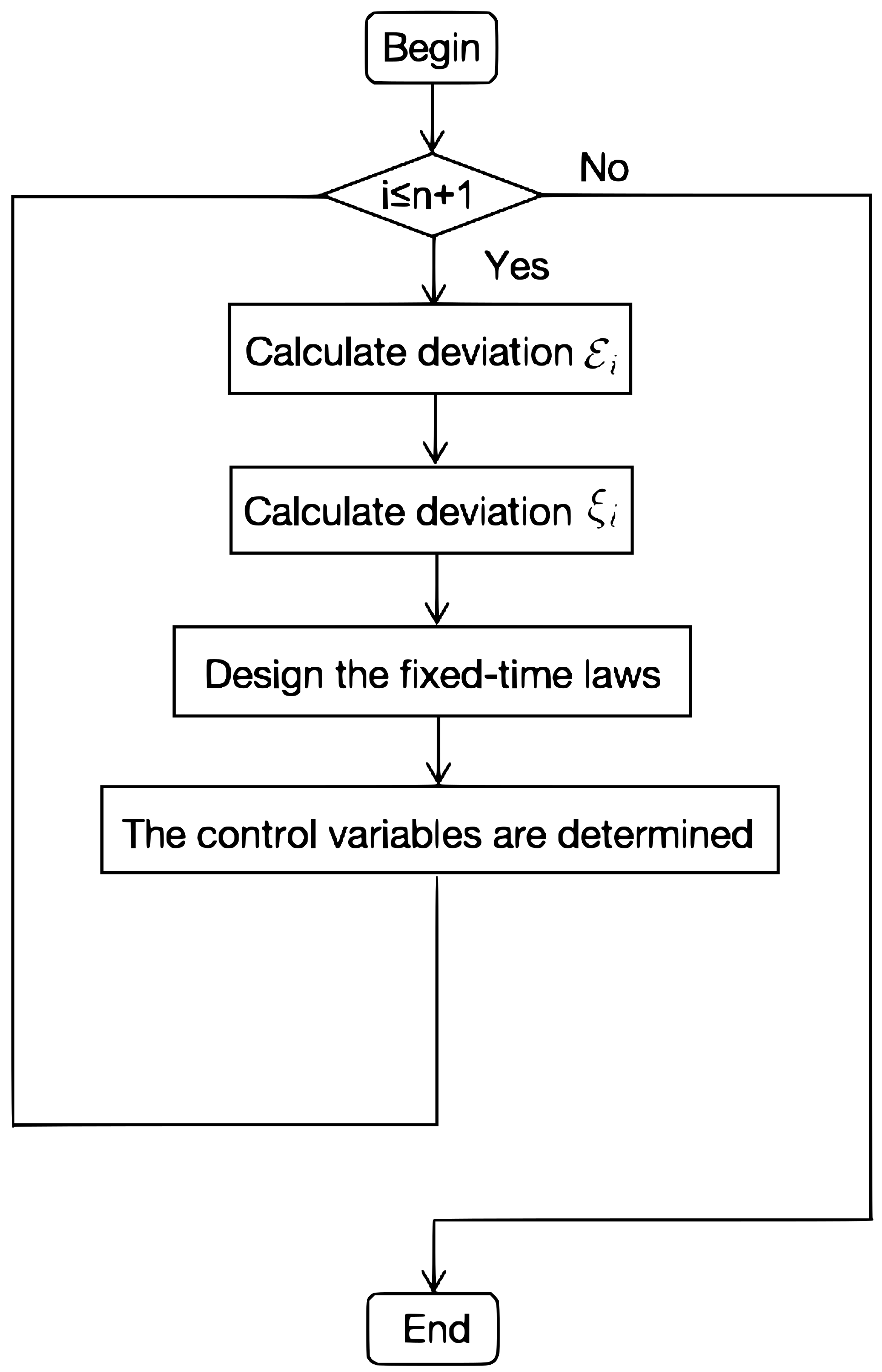
The flow chart of the fixed-time control algorithm in this section is shown in Figure 1 below.

Figure 1.
The fixed-time control algorithm.
4. Simulation
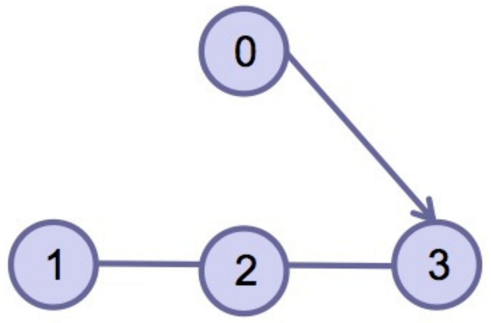
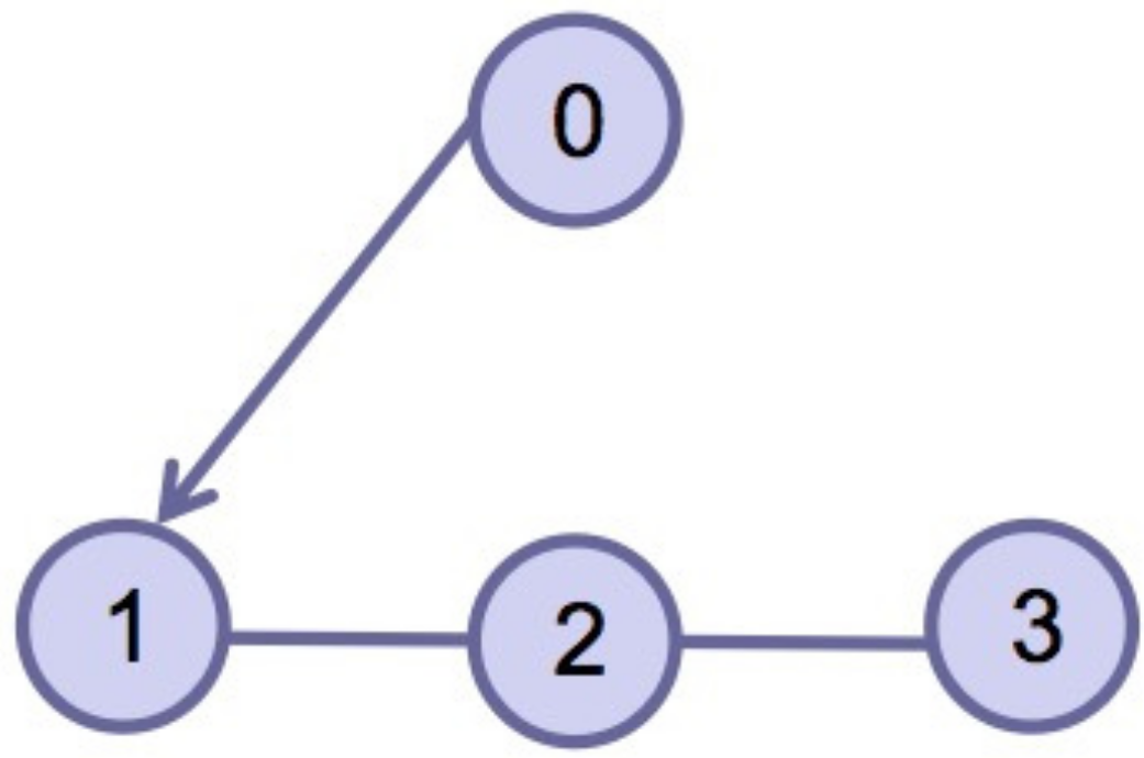
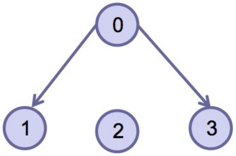
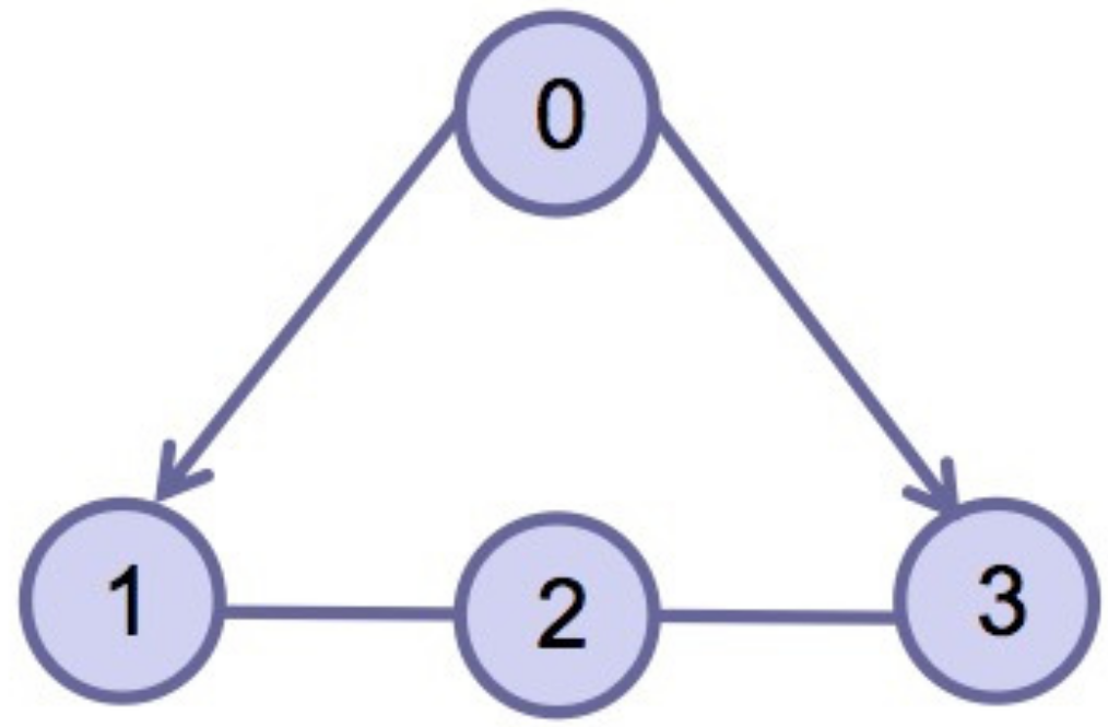
This section verifies the validity of the theoretical results through a simulation example. Consider four agents, one of which acts as the leader and is numbered 0, and the other three act as followers and are numbered 1–3. The dynamics of the four agents is shown in (2) and (3). Choose interval and ; namely, interval is divided into three sub-intervals , , , , , the subgraph of each sub-time interval is shown in Figure 2, Figure 3 and Figure 4. The jointly connected graph of the three subgraphs is shown in Figure 5.
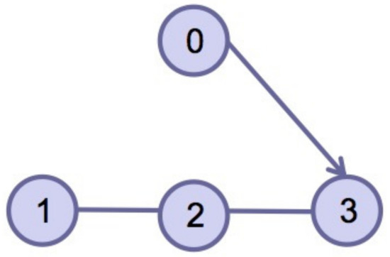
Figure 2.
Subgraph in sub-interval .
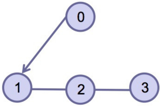
Figure 3.
Subgraph in sub-interval .
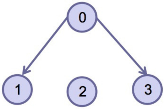
Figure 4.
Subgraph in sub-interval .
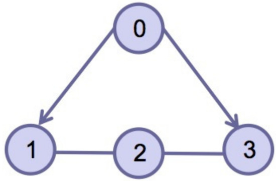
Figure 5.
The jointly connected graph in time interval .
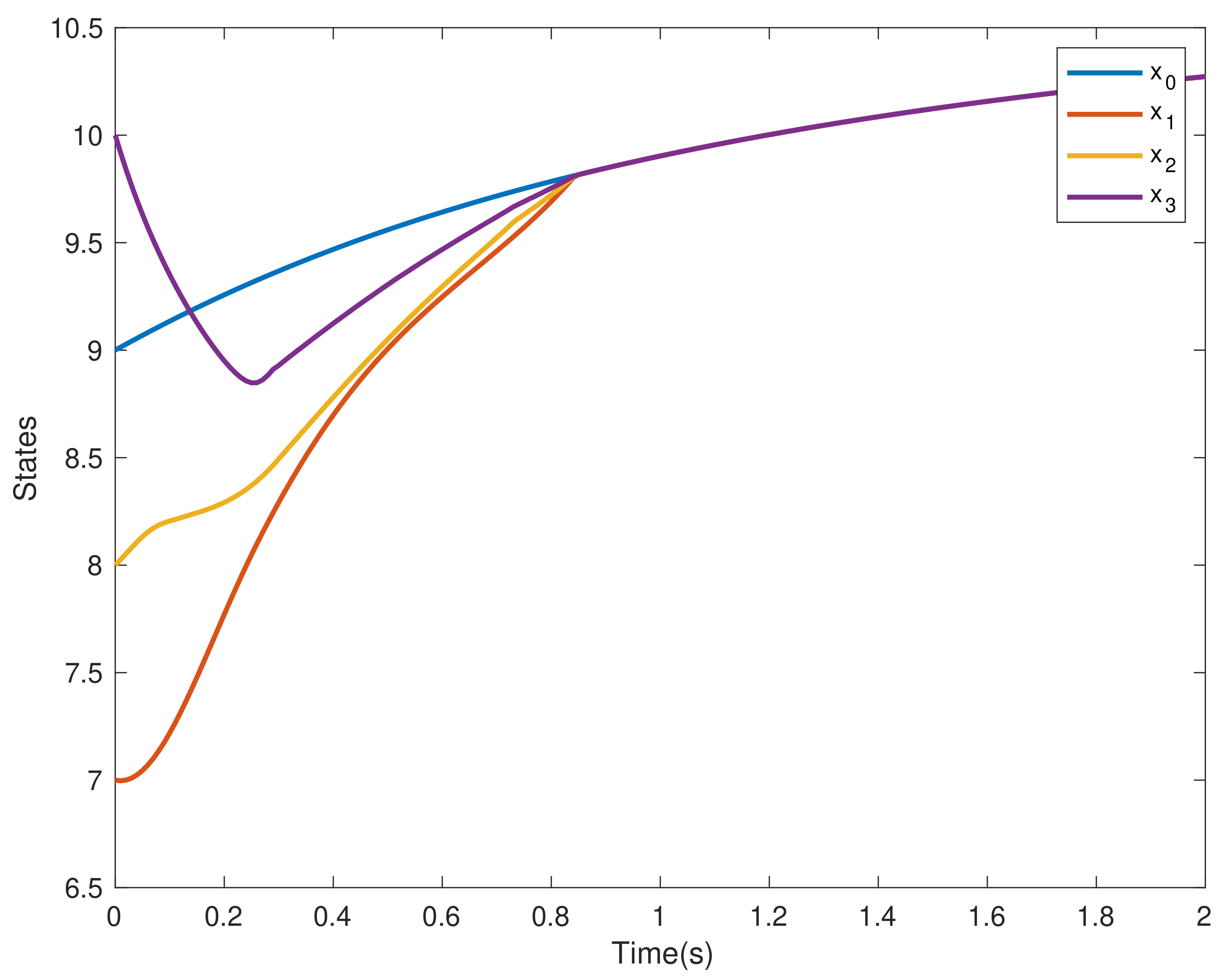
Furthermore, the initial value of the leader is , and the initial value of the followers is , while the adjacency matrix and the Laplacian matrix associated with Figure 5 are shown in (29) and (30). In addition, the nonlinear term of the leader is described by , and the nonlinear terms of followers are described by , and , respectively. Uncertain disturbances are regarded as , and , respectively. Finally, let , , and .
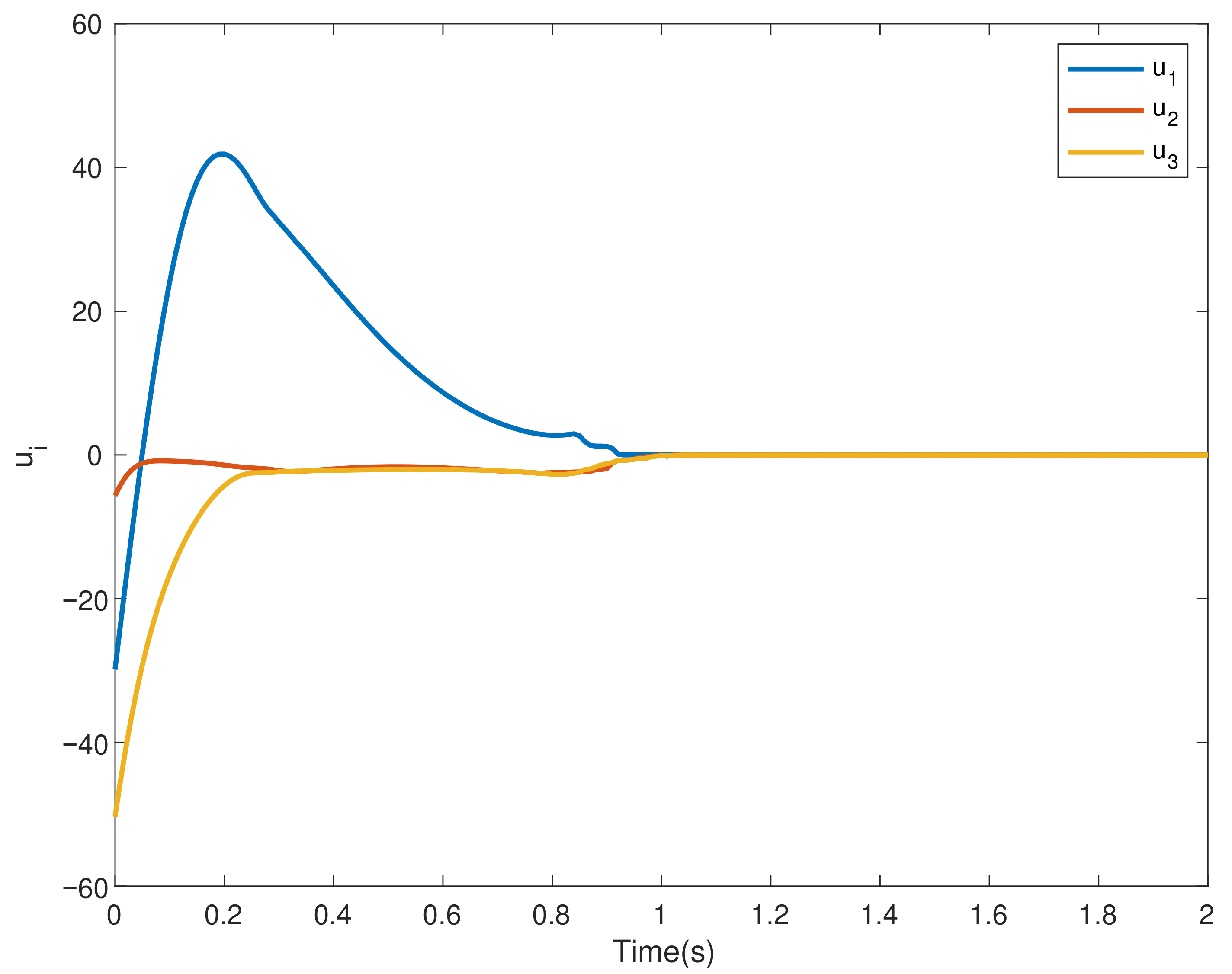
In the multi-agent systems composed of four agents, under the control (4), the states of the followers successfully converge to that of the leader agent within a fixed time independent of the initial value, as shown in Figure 6. The trajectories of consensus errors and the control inputs of each followers are given by Figure 7 and Figure 8, respectively.

Figure 6.
The states trajectories of the agents .
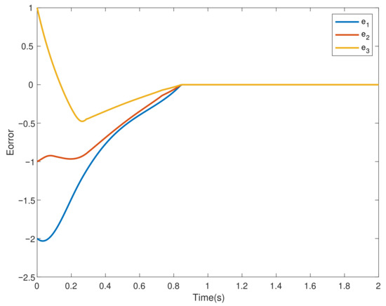
Figure 7.
Trajectories of consensus errors .
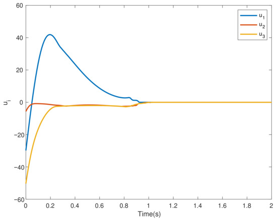
Figure 8.
The control inputs .
5. Conclusions
In this paper, we research how to achieve fixed-time leader-following consensus for nonlinear multi-agent systems under a jointly connected graph. In addition, the system is affected by unknown disturbances. Compared with other studies in the literature on the fixed-time consensus problem, the advantage of this paper is that the unknown nonlinearity and unknown disturbances in the multi-agent systems can be solved under the jointly connected graph, simultaneously. Finally, this paper uses Matlab to carry out numerical simulation, which provides with a more intuitive proof of the theoretical part. In the future, the fixed time consensus problem of high-order nonlinear multi-agent systems can be solved.
Author Contributions
Conceptualization, M.Z.; Data curation, M.Z.; Formal analysis, C.G. and L.Z.; Funding acquisition, C.G. and Y.L.; Project administration, C.G.; Supervision, Y.L.; Validation, L.Z. and Y.L.; Visualization, C.G.; Writing—original draft, M.Z.; Writing—review & editing, L.Z. All authors have read and agreed to the published version of the manuscript.
Funding
This work was sponsored in part by the National Natural Science Foundation of China under Grant No. 62003201.
Institutional Review Board Statement
Not applicable.
Informed Consent Statement
Not applicable.
Data Availability Statement
Not applicable.
Conflicts of Interest
The authors declare no conflict of interest.
References
- Han, T.; Chi, M.; Guan, Z.H.; Hu, B.; Xiao, J.W.; Huang, Y. Distributed Three-Dimensional Formation Containment Control of Multiple Unmanned Aerial Vehicle Systems: Distributed 3D Formation Containment Control of Multiple UAV Systems. Asian J. Control 2017, 19, 1103–1113. [Google Scholar] [CrossRef]
- Loria, A.; Dasdemir, J.; Jarquin, N.A. Leader–follower formation and tracking control of mobile robots along straight paths. IEEE Trans. Control Syst. Technol. 2015, 24, 727–732. [Google Scholar] [CrossRef]
- Minsky, M. The Society of Mind; JSTOR: New York, NY, USA, 1987. [Google Scholar]
- Zhang, S.; Tepedelenlioǧlu, C.; Banavar, M.K.; Spanias, A. Max consensus in sensor networks: Non-linear bounded transmission and additive noise. IEEE Sens. J. 2016, 16, 9089–9098. [Google Scholar] [CrossRef]
- Jiang, J.; Jiang, Y. Leader-following consensus of linear time-varying multi-agent systems under fixed and switching topologies. Automatica 2020, 113, 108804. [Google Scholar] [CrossRef]
- Li, Z.; Duan, Z. Cooperative Control of Multi-Agent Systems: A Consensus Region Approach; CRC Press: Boca Raton, FL, USA, 2017. [Google Scholar]
- Guan, Z.H.; Sun, F.L.; Wang, Y.W.; Li, T. Finite-time consensus for leader-following second-order multi-agent networks. IEEE Trans. Circuits Syst. I Regul. Pap. 2012, 59, 2646–2654. [Google Scholar] [CrossRef]
- Li, S.; Du, H.; Lin, X. Finite-time consensus algorithm for multi-agent systems with double-integrator dynamics. Automatica 2011, 47, 1706–1712. [Google Scholar] [CrossRef]
- Wang, L.; Xiao, F. Finite-time consensus problems for networks of dynamic agents. IEEE Trans. Autom. Control 2010, 55, 950–955. [Google Scholar] [CrossRef]
- Zhao, L.; Liu, Y.; Li, F.; Man, Y. Fully distributed adaptive finite-time consensus for uncertain nonlinear multiagent systems. IEEE Trans. Cybern. 2010, 52, 6972–6983. [Google Scholar] [CrossRef]
- Asiri, S.; Liu, D.Y. Finite-time estimation for a class of systems with unknown time-delay using modulating functions-based method. Asian J. Control 2022. [Google Scholar] [CrossRef]
- Li, Y.; Yang, R. Distributed finite-time formation of networked nonlinear systems via dynamic gain control. Asian J. Control 2022. [Google Scholar] [CrossRef]
- Van, M.; Sam Ge, S.; Ceglarek, D. Global finite-time cooperative control for multiple manipulators using integral sliding mode control. Asian J. Control 2021. [Google Scholar] [CrossRef]
- Polyakov, A. Nonlinear feedback design for fixed-time stabilization of linear control systems. IEEE Trans. Autom. Control 2011, 57, 2106–2110. [Google Scholar] [CrossRef]
- Zuo, Z. Nonsingular fixed-time consensus tracking for second-order multi-agent networks. Automatica 2015, 54, 305–309. [Google Scholar] [CrossRef]
- Tian, B.; Lu, H.; Zuo, Z.; Yang, W. Fixed-time leader–follower output feedback consensus for second-order multiagent systems. IEEE Trans. Cybern. 2018, 49, 1545–1550. [Google Scholar] [CrossRef]
- Defoort, M.; Polyakov, A.; Demesure, G.; Djemai, M.; Veluvolu, K. Leader-follower fixed-time consensus for multi-agent systems with unknown non-linear inherent dynamics. IET Control Theory Appl. 2015, 9, 2165–2170. [Google Scholar] [CrossRef]
- Hong, H.; Yu, W.; Wen, G.; Yu, X. Distributed robust fixed-time consensus for nonlinear and disturbed multiagent systems. IEEE Trans. Syst. Man Cybern. Syst. 2016, 47, 1464–1473. [Google Scholar] [CrossRef]
- Shang, Y. Fixed-time group consensus for multi-agent systems with non-linear dynamics and uncertainties. IET Control Theory Appl. 2018, 12, 395–404. [Google Scholar] [CrossRef]
- You, X.; Hua, C.; Li, K.; Jia, X. Fixed-time leader-following consensus for high-order time-varying nonlinear multiagent systems. IEEE Trans. Autom. Control 2020, 65, 5510–5516. [Google Scholar] [CrossRef]
- Liu, Y.; Zhao, Y.; Ren, W.; Chen, G. Appointed-time consensus: Accurate and practical designs. Automatica 2018, 89, 425–429. [Google Scholar] [CrossRef]
- Zhao, L.; Sun, Y.; Dai, H.; Zhao, D. Stochastic fixed-time consensus problem of multi-agent systems with fixed and switching topologies. Int. J. Control 2021, 94, 2811–2821. [Google Scholar] [CrossRef]
- Cui, L.; Zhou, Q.; Jin, N. Fixed-time backstepping distributed cooperative control for multiple unmanned aerial vehicles. Asian J. Control 2022. [Google Scholar] [CrossRef]
- Yao, Q. Fixed-time adaptive neural control for nonstrict-feedback uncertain nonlinear systems with output constraints. Asian J. Control 2022. [Google Scholar] [CrossRef]
- Chen, M.; Wang, H.; Liu, X. Adaptive Fuzzy Practical Fixed-Time Tracking Control of Nonlinear Systems. Daptive Fuzzy Pract. Fixed-Time Track. Control Nonlinear Syst. 2021, 29, 664–673. [Google Scholar] [CrossRef]
- Yan, C.; Amir, R.; Ardashir, M.; Sakthivel, R. Deep learned recurrent type-3 fuzzy system: Application for renewable energy modeling/prediction. Energy Rep. 2021, 7, 8115–8127. [Google Scholar]
- Wei, X.; Yu, W.; Wang, H.; Yao, Y.; Mei, F. An observer-based fixed-time consensus control for second-order multi-agent systems with disturbances. IEEE Trans. Circuits Syst. II Express Briefs 2018, 66, 247–251. [Google Scholar] [CrossRef]
- Zuo, Z.; Tian, B.; Defoort, M.; Ding, Z. Fixed-time consensus tracking for multiagent systems with high-order integrator dynamics. IEEE Trans. Autom. Control 2017, 63, 563–570. [Google Scholar] [CrossRef]
- Xu, Y.; Yao, Z.; Lu, R.; Ghosh, B. A novel fixed-time protocol for first-order consensus tracking with disturbance rejection. IEEE Trans. Autom. Control 2021. [Google Scholar] [CrossRef]
- Tian, B.; Shao, X.; Yang, W.; Zhang, W. Fixed time output feedback containment for uncertain nonlinear multiagent systems with switching communication topologies. ISA Trans. 2021, 111, 82–95. [Google Scholar]
- Parsegov, S.; Polyakov, A.; Shcherbakov, P. Fixed-time consensus algorithm for multi-agent systems with integrator dynamics. IFAC Proc. Vol. 2013, 46, 110–115. [Google Scholar] [CrossRef]
- Hardy, G.H.; Littlewood, J.E.; Polya, G. Inequalities; Cambridge University Press: Cambridge, UK, 1952. [Google Scholar]
- Ren, W.; Beard, R.W. Consensus seeking in multiagent systems under dynamically changing interaction topologies. IEEE Trans. Autom. Control 2005, 50, 655–661. [Google Scholar] [CrossRef]

Publisher’s Note: MDPI stays neutral with regard to jurisdictional claims in published maps and institutional affiliations. |
© 2022 by the authors. Licensee MDPI, Basel, Switzerland. This article is an open access article distributed under the terms and conditions of the Creative Commons Attribution (CC BY) license (https://creativecommons.org/licenses/by/4.0/).