

A Neural Network-Based Mesh Quality Indicator for Three-Dimensional Cylinder Modelling

Abstract
:1. Introduction
2. Related Works
2.1. Traditional Mesh Quality Indicators
2.2. Neural Networks for Mesh Quality Evaluation
3. A Neural Network-Based Mesh Quality Indicator for Three-Dimensional Cylinder Modelling
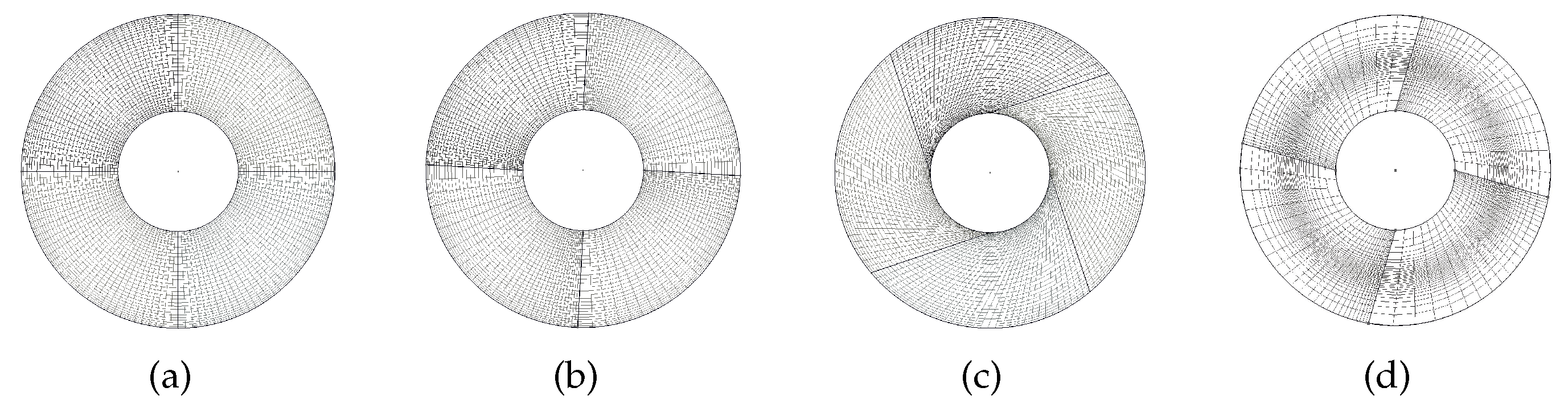
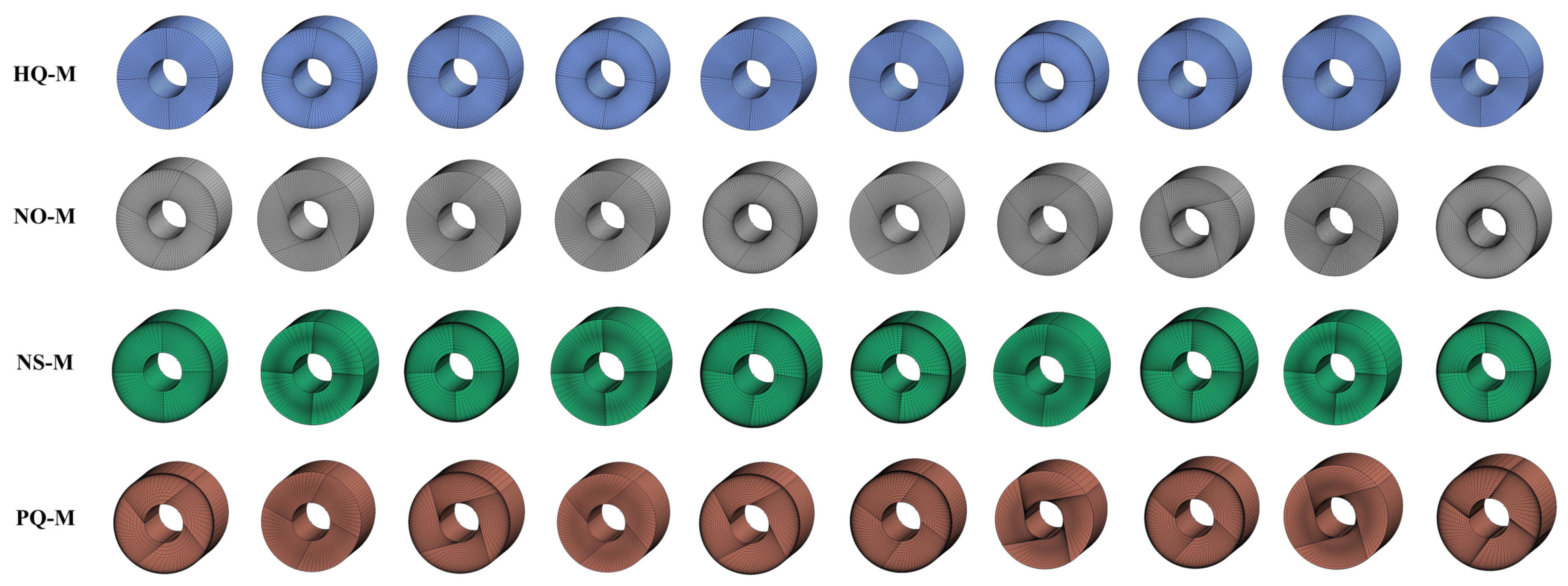
3.1. Three-Dimensional Cylinder Mesh Benchmark Dataset
- (1)
- High-quality Mesh: is a class of acceptable meshes with a very small error in the numerical solution.
- (2)
- Non-orthogonal Mesh: occurs when the curves or surfaces of the mesh are not vertically orthogonal. Numerical experiments in [5] show that skewed mesh with poor orthogonality can affect the order of accuracy and error magnitude. Non-orthogonal meshes also have a negative impact on the convergence speed.
- (3)
- (4)
- Poor-quality Mesh: represents meshes with poor orthogonality, smoothness, and distribution. According to the analysis in [34], poorly-shaped meshes can cause the ill-conditioned stiffness matrix problem and seriously affect the solutions of the partial differential equations.
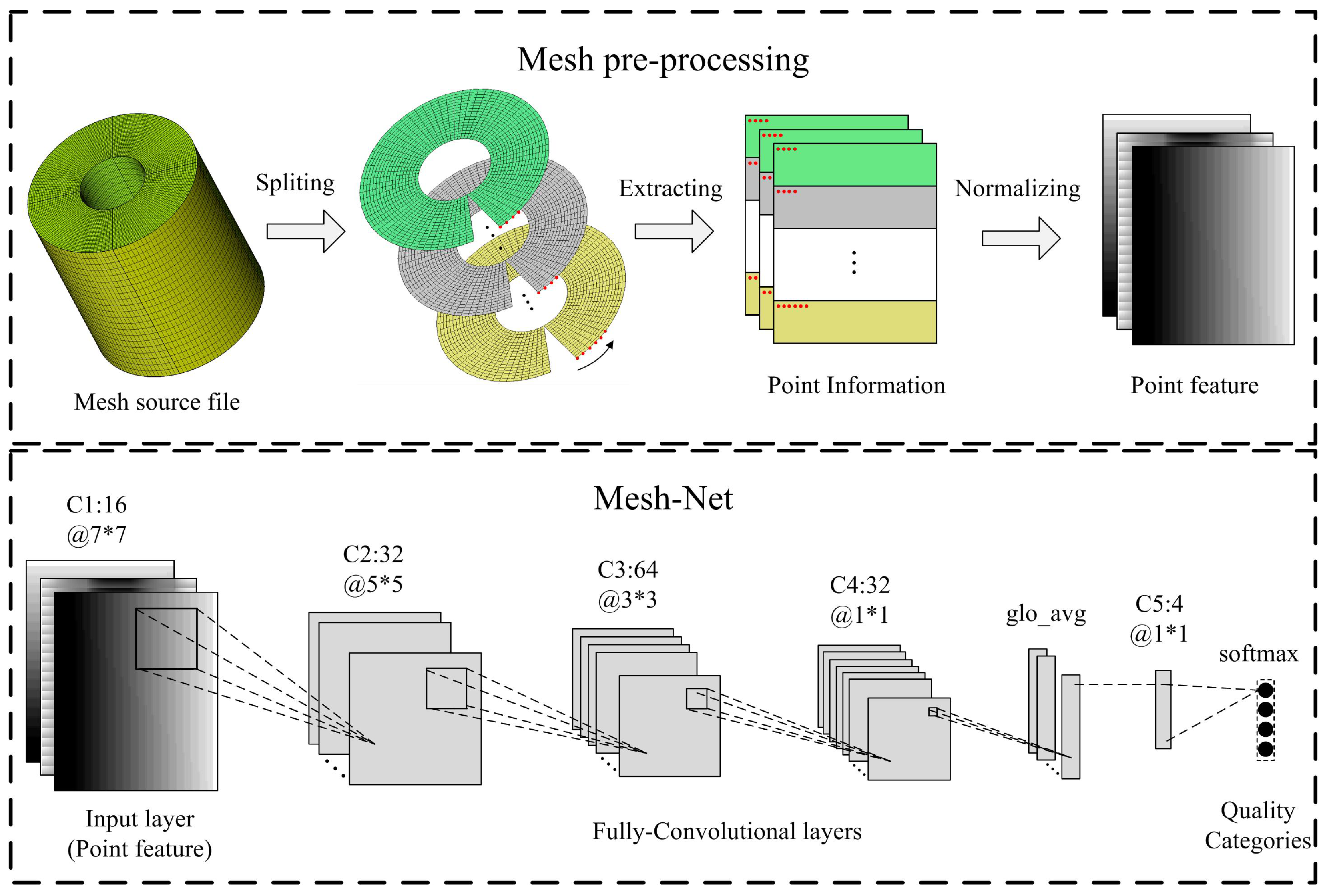
3.2. Mesh Pre-Processing
3.3. The Structure of Mesh-Net
4. Experimental Results and Discussions
4.1. Training
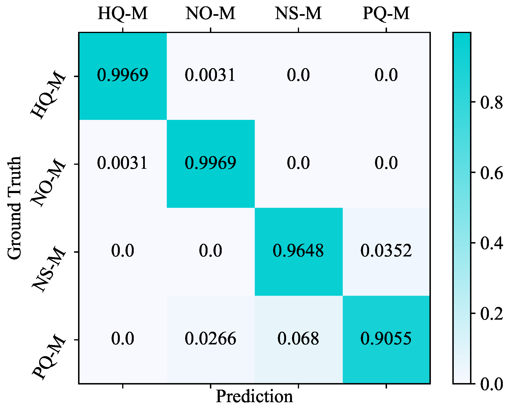
4.2. Prediction
5. Conclusions
Author Contributions
Funding
Data Availability Statement
Conflicts of Interest
References
- Chen, X.; Liu, J.; Li, S.; Xie, P.; Chi, L.; Wang, Q. TAMM: A New Topology-Aware Mapping Method for Parallel Applications on the Tianhe-2A Supercomputer. In Algorithms and Architectures for Parallel Processing; Vaidya, J., Li, J., Eds.; Springer International Publishing: Cham, Switzerland, 2018; pp. 242–256. [Google Scholar]
- Garimella, R.V.; Shashkov, M.; Knupp, P.M. Triangular and quadrilateral surface mesh quality optimization using local parametrization. Comput. Methods Appl. Mech. Eng. 2004, 193, 913–928. [Google Scholar] [CrossRef]
- Shi, R.; Lin, J.; Yang, H. Numerical Study on the Coagulation and Breakage of Nanoparticles in the Two-Phase Flow around Cylinders. Entropy 2022, 24, 526. [Google Scholar] [CrossRef] [PubMed]
- Chen, X.; Li, T.; Wan, Q.; He, X.; Gong, C.; Pang, Y.; Liu, J. MGNet: A novel differential mesh generation method based on unsupervised neural networks. Eng. Comput. 2022, 1–13. [Google Scholar] [CrossRef]
- Blacker, T.D.; Owen, S.J.; Staten, M.L.; Quadros, W.R.; Hanks, B.; Clark, B.W.; Meyers, R.J.; Ernst, C.; Merkley, K.; Morris, R.; et al. CUBIT Geometry and Mesh Generation Toolkit 15.1 User Documentation; U.S. Department of Energy Office of Scientific and Technical Information: Washington, DC, USA, 2016. [CrossRef]
- Berzins, M. Mesh Quality: A Function of Geometry, Error Estimates or Both? Eng. Comput. 1999, 15, 236–247. [Google Scholar] [CrossRef]
- Katz, A.; Sankaran, V. Mesh quality effects on the accuracy of CFD solutions on unstructured meshes. J. Comput. Phys. 2011, 230, 7670–7686. [Google Scholar] [CrossRef]
- Lowrie, W.; Lukin, V.S.; Shumlak, U. A Priori Mesh Quality Metric Error Analysis Applied to a High-Order Finite Element Method. J. Comput. Phys. 2011, 230, 5564–5586. [Google Scholar] [CrossRef]
- Chen, X.; Liu, J.; Pang, Y.; Chen, J.; Chi, L.; Gong, C. Developing a new mesh quality evaluation method based on convolutional neural network. Eng. Appl. Comput. Fluid Mech. 2020, 14, 391–400. [Google Scholar] [CrossRef]
- Diskin, B.; Thomas, J. Effects of mesh regularity on accuracy of finite-volume schemes. In Proceedings of the 50th AIAA Aerospace Sciences Meeting Including the New Horizons Forum and Aerospace Exposition, Nashville, TN, USA, 9–12 January 2012. [Google Scholar] [CrossRef]
- Lo, S. Optimization of tetrahedral meshes based on element shape measures. Comput. Struct. 1997, 63, 951–961. [Google Scholar] [CrossRef]
- Huang, Y.; Liupeng, W.; Yi, N. Mesh Quality and More Detailed Error Estimates of Finite Element Method. Numer. Math. Theory, Methods Appl. 2017, 10, 420–436. [Google Scholar] [CrossRef]
- Nie, C.; Liu, J.; Sun, S. Study on quality measures fpr tetrahedral mesh. Chin. J. Comput. Mech. 2003, 20, 579–582. [Google Scholar]
- Gao, X.; Huang, J.; Xu, K.; Pan, Z.; Deng, Z.; Chen, G. Evaluating Hex-mesh Quality Metrics via Correlation Analysis. Comput. Graph. Forum 2017, 36, 105–116. [Google Scholar] [CrossRef]
- Hu, J.; Shen, L.; Sun, G. Squeeze-and-excitation networks. In Proceedings of the IEEE Conference on Computer Vision and Pattern Recognition, Salt Lake City, UT, USA, 18–23 June 2018; pp. 7132–7141. [Google Scholar]
- Sandler, M.; Howard, A.; Zhu, M.; Zhmoginov, A.; Chen, L.C. Mobilenetv2: Inverted residuals and linear bottlenecks. In Proceedings of the IEEE Conference on Computer Vision and Pattern Recognition, Salt Lake City, UT, USA, 18–23 June 2018; pp. 4510–4520. [Google Scholar]
- Li, M.; Li, S.; Zhang, J.; Wu, F.; Zhang, T. Neural Adaptive Funnel Dynamic Surface Control with Disturbance-Observer for the PMSM with Time Delays. Entropy 2022, 24, 1028. [Google Scholar] [CrossRef] [PubMed]
- Ray, D.; Hesthaven, J.S. An artificial neural network as a troubled-cell indicator. J. Comput. Phys. 2018, 367, 166–191. [Google Scholar] [CrossRef]
- Knupp, P.M. Achieving finite element mesh quality via optimization of the Jacobian matrix norm and associated quantities. Part I—A framework for surface mesh optimization. Int. J. Numer. Methods Eng. 2000, 48, 401–420. [Google Scholar] [CrossRef]
- Geuzaine, C.; Remacle, J.F. Gmsh: A three-dimensional finite element mesh generator with built-in pre- and post-processing facilities. Int. J. Numer. Methods Eng. 2009, 11, 1309–1331. [Google Scholar] [CrossRef]
- Strang, G.; Fix, G. An Analysis of The Finite Element Method. J. Appl. Mech. 1973, 41, 62. [Google Scholar] [CrossRef]
- Shewchuk, J.R. Delaunay refinement algorithms for triangular mesh generation. Comput. Geom. 2002, 22, 21–74. [Google Scholar] [CrossRef]
- Liu, A.; Joe, B. Relationship between tetrahedron shape measures. BIT Numer. Math. 1994, 34, 268–287. [Google Scholar] [CrossRef]
- Bank, R.E.; Smith, R.K. Mesh Smoothing Using A Posteriori Error Estimates. SIAM J. Numer. Anal. 1997, 34, 979–997. [Google Scholar] [CrossRef] [Green Version]
- Weatherill, N.P.; Morgan, K.; Hassan, O.; Jones, J.W. Large-scale aerospace simulations using unstructured grid technology. In Computational Mechanics for the Twenty-First Century; Civil-Comp Press: Edinburgh, UK, 2000. [Google Scholar]
- Antiga, L.; Ene-Iordache, B.; Caverni, L.; Cornalba, G.P.; Remuzzi, A. Geometric reconstruction for computational mesh generation of arterial bifurcations from CT angiography. Comput. Med. Imaging Graph. 2002, 26, 227–235. [Google Scholar] [CrossRef]
- Chong, C.S.; Lee, H.P.; Kumar, A.S. Genetic algorithms in mesh optimization for visualization and finite element models. Neural Comput. Appl. 2006, 15, 366–372. [Google Scholar] [CrossRef]
- Mall, S.; Chakraverty, S. Comparison of Artificial Neural Network Architecture in Solving Ordinary Differential Equations. Adv. Artif. Neural Syst. 2013, 2013, 181895. [Google Scholar] [CrossRef]
- Tan, M.; Le, Q.V. Efficientnet: Rethinking model scaling for convolutional neural networks. In Proceedings of the International Conference on Machine Learning, Long Beach, CA, USA, 9–15 June 2019. [Google Scholar]
- Chen, X.; Liu, J.; Gong, C.; Pang, Y.; Chen, B. An Airfoil Mesh Quality Criterion using Deep Neural Networks. In Proceedings of the 12th International Conference on Advanced Computational Intelligence, Dali, China, 14–16 August 2020; pp. 536–541. [Google Scholar]
- Chen, X.; Gong, C.; Liu, J.; Pang, Y.; Liang, D.; Chi, L.; Li, K. A Novel Neural Network Approach for Airfoil Mesh Quality Evaluation. J. Parallel Distrib. Comput. 2022, 164, 123–132. [Google Scholar] [CrossRef]
- Farwig, R. An Lq-analysis of viscous fluid flow past a rotating obstacle. Tohoku Math. J. 2006, 58, 129–147. [Google Scholar] [CrossRef]
- Knupp, P.M. Matrix Norms and the Condition Number: A General Framework to Improve Mesh Quality via Node-Movement. Off. Sci. Tech. Inf. Tech. Rep. 1999, 36, 13–22. [Google Scholar]
- Zhang, Y.; Jia, Y.; Wang, S.S.Y. Structured mesh generation with smoothness controls. Int. J. Numer. Methods Fluids 2006, 51, 1255–1276. [Google Scholar] [CrossRef]
- Qi, C.R.; Su, H.; Mo, K.; Guibas, L.J. Pointnet: Deep learning on point sets for 3d classification and segmentation. In Proceedings of the IEEE Conference on Computer Vision and Pattern Recognition, Honolulu, HI, USA, 21–26 July 2017; pp. 652–660. [Google Scholar]
- Abadi, M.; Barham, P.; Chen, J.; Chen, Z.; Davis, A.; Dean, J.; Devin, M.; Ghemawat, S.; Irving, G.; Isard, M.; et al. TensorFlow: A System for Large-Scale Machine Learning. In Proceedings of the 12th USENIX Conference on Operating Systems Design and Implementation, Savannah, GA, USA, 2–4 November 2016; USENIX Association: Berkeley, CA, USA, 2016; pp. 265–283. [Google Scholar]


| Parameter | Value |
|---|---|
| Density | 1 kg/m |
| Viscosity | 0.0002 kg/m |
| Radius of the inner cylinder | 17.8 mm |
| Radius of the outer cylinder | 46.28 mm |
| Angular velocity of the inner wall | 1 rad/s |
| Case | Mesh Size | Number of Meshes |
|---|---|---|
| Size 1 | 96 × 30 × 20 | 2048 |
| Size 2 | 100 × 30 × 20 | 2048 |
| Size 3 | 104 × 30 × 20 | 2048 |
| Size 4 | 108 × 30 × 20 | 2048 |
| Size 5 | 112 × 31 × 20 | 2048 |
| Size 6 | 116 × 31 × 20 | 2048 |
| Size 7 | 120 × 31 × 20 | 2048 |
| Size 8 | 124 × 31 × 20 | 2048 |
| Size 9 | 128 × 32 × 21 | 2048 |
| Size 10 | 132 × 32 × 21 | 2048 |
| Label | Quality Categories | Number of Meshes |
|---|---|---|
| 1 (HQ-M) | High-quality Mesh | 512 × 10 |
| 2 (NO-M) | Non-orthogonal Mesh | 512 × 10 |
| 3 (NS-M) | Non-smoothness Mesh | 512 × 10 |
| 4 (PQ-M) | Poor-quality Mesh | 512 × 10 |
| Case | Model | Accuracy (%) |
|---|---|---|
| Size 1 test | SVM | 89.06% |
| QDA | 87.30% | |
| GNB | 79.49% | |
| MLP | 95.70% | |
| Mesh-Net | 98.05% | |
| Full-size test | Mesh-Net | 96.60% |
Publisher’s Note: MDPI stays neutral with regard to jurisdictional claims in published maps and institutional affiliations. |
© 2022 by the authors. Licensee MDPI, Basel, Switzerland. This article is an open access article distributed under the terms and conditions of the Creative Commons Attribution (CC BY) license (https://creativecommons.org/licenses/by/4.0/).
Share and Cite
Chen, X.; Wang, Z.; Liu, J.; Gong, C.; Pang, Y. A Neural Network-Based Mesh Quality Indicator for Three-Dimensional Cylinder Modelling. Entropy 2022, 24, 1245. https://doi.org/10.3390/e24091245
Chen X, Wang Z, Liu J, Gong C, Pang Y. A Neural Network-Based Mesh Quality Indicator for Three-Dimensional Cylinder Modelling. Entropy. 2022; 24(9):1245. https://doi.org/10.3390/e24091245
Chicago/Turabian StyleChen, Xinhai, Zhichao Wang, Jie Liu, Chunye Gong, and Yufei Pang. 2022. "A Neural Network-Based Mesh Quality Indicator for Three-Dimensional Cylinder Modelling" Entropy 24, no. 9: 1245. https://doi.org/10.3390/e24091245
APA StyleChen, X., Wang, Z., Liu, J., Gong, C., & Pang, Y. (2022). A Neural Network-Based Mesh Quality Indicator for Three-Dimensional Cylinder Modelling. Entropy, 24(9), 1245. https://doi.org/10.3390/e24091245