Abstract
We consider the problem of transmitting a Gaussian source with minimum mean square error distortion over an infinite-bandwidth additive white Gaussian noise channel with an unknown noise level and under an input energy constraint. We construct a universal joint source–channel coding scheme with respect to the noise level, that uses modulo-lattice modulation with multiple layers. For each layer, we employ either analog linear modulation or analog pulse-position modulation (PPM). We show that the designed scheme with linear layers requires less energy compared to existing solutions to achieve the same quadratically increasing distortion profile with the noise level; replacing the linear layers with PPM layers offers an additional improvement.
1. Introduction
Due to the recent technological advancements in sensing technology and the internet of things, there is a growing demand for low-energy communications solutions. Indeed, since many of the sensors have only limited batteries due to environmental (in the case of energy harvesting) or replenishment limitations, these solutions need to be economical in terms of the utilized energy. Moreover, since each sensor may serve several parties, with each experiencing different conditions, these solutions need to be robust with respect to the noise level.
This problem may be conveniently modeled as the classical setup of conveying k independent and identically distributed (i.i.d.) Gaussian source samples with minimum mean square error (MMSE) distortion over a continuous-time additive white Gaussian noise (AWGN) channel under a channel input total energy constraint , where E is the allowed transmit energy per source sample and unconstrained transmit bandwidth; see Figure 1.
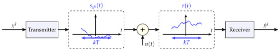
Figure 1.
JSCC of k samples of a Gaussian source, , over a continuous-time bandwidth-unlimited AWGN channel subject to an energy constraint (8). The noise level of the noise process n is assumed to be known only to the receiver but not to the transmitter. The transmitter maps the k source samples into a continuous-time channel input (and arbitrarily large bandwidth). The receiver constructs an estimate of from the continuous-time channel output .
For the encapsulated source–coding problem for a large k, the optimal tradeoff between the compression rate R and the (per-sample) MMSE distortion D [1] (Chapter 13.2) for a memoryless Gaussian source with variance is dictated by the rate–distortion function [1] (Chapter 13.3):
where is the signal-to-distortion ratio (SDR).
For the encapsulated channel-coding problem, since the bandwidth is unconstrained (i.e., grows to infinity), and the allowed energy of the channel input is constrained by E, the maximal achievable total reliable rate (in nats) of the entire transmission—the total capacity—is given by [1] (Chapter 9.3)
when the power spectral density of the noise (the noise level) N is known to the transmitter (and the receiver), and where is the energy-to-noise ratio. We note that, in our setting, the transmit energy E is fixed regardless of the transmission duration and bandwidth, in contrast to the power-limited setting, in which the energy grows linearly with the transmission time for a fixed power P. To emphasize this, following [2,3] and others, we make use of to distinguish it from the more common signal-to-noise ratio (SNR), which is defined in the fixed-power scenario as .
Returning to the overall problem of conveying k i.i.d. source samples of a Gaussian source over a continuous-time AWGN channel subject to an energy constraint (and unconstrained bandwidth), in the limit of a large-source blocklength k, the optimal achievable mean square error distortion per source sample is dictated by the celebrated source–channel separation principle [1] (Th. 10.4.1), [4] (Chapter 3.9): , which upon substituting (1) and (2), amounts to
For non-Gaussian continuous memoryless sources, the optimal distortion is bounded as [1] (Prob. 10.8, Th. 10.4.1), [4] (Prob. 3.18, Chapter 3.9)
where the lower bound stems from Shannon’s lower bound [5], the upper bound holds since a Gaussian source is the “least compressable” source with a given variance under a quadratic distortion measure, and denotes the differential entropy of a sample of the i.i.d. source x [1] (Chapter 8), [4] (Chapter 2.2).
While the optimal performance is known when the transmitter (and the receiver) knows the noise level and , determining it becomes much more challenging when the noise level is unknown at the transmitter. Indeed, when the transmitter is oblivious of the true noise level, achieving (3) for all noise levels simultaneously is impossible [6,7]. Instead, one wishes to achieve graceful degradation of the distortion with the noise level, namely, a scheme that would work well for a continuum of all possible noise levels without knowing the true noise level at the transmitter. Since the distortion improves exponentially with the ENR (3) when the noise level is known, in the absence of knowledge of the noise level at the transmitter, one might hope to attain an exponential distortion decay profile with the ENR of the form
for some , or, equivalently,
for some and some finite per-sample energy E. Köken and Tuncel [7] proved that, unfortunately, this is impossible, namely, no (equivalently and ) exist for which (5a,b) is achievable simultaneously for all (equivalently, for all ). Consequently, distortion profiles that deteriorate faster with the noise level need to be sought.
For the case of finite bandwidth expansion/compression B (and finite power), by superimposing digital successive refinements [8] with a geometric power allocation, Santhi and Vardy [9,10] and Bhattad and Narayanan [11] showed that, in our terms, the distortion improves like for an arbitrarily small , for large ENR values. This suggests that by taking the bandwidth to be large enough, a polynomial decay with an of any finite degree, however large, is achievable, starting from a large enough ENR. In our setting of interest, in which the bandwidth is unconstrained, this means, in turn, that there exists a finite energy E for which a polynomially decaying distortion profile in N
is attainable for any predetermined power , however large yet finite, and for any predetermined constant of our choice, with large enough finite per-sample energy ; for the particular choice of for any constant of our choice, this is equivalent to
Mittal and Phamdo [12] constructed a different scheme, that works above a certain minimum (not necessarily large) design ENR by sending the digital successive refinements incrementally over non-overlapping frequency bands, and sending the quantization error r of the last digital refinement over the last frequency band.
The scheme of Mittal and Phamdo was subsequently improved by Reznic et al. [6] (see also [13,14], [15] (Chapter 11.1)) by replacing the successive refinement layers with lattice-based Wyner–Ziv coding [16,17], [4] (Chapter 11.3) which, in contrast to the digital layers of the scheme of Mittal and Phamdo, enjoys an improvement in each of the layers with the ENR.
Kokën and Tuncel [7] adopted the scheme of Mittal and Phamdo in the infinite-bandwidth (and infinite-blocklength) setting. Baniasadi and Tuncel [18] (see also [19]) further improved this scheme by allowing the sending of the resulting analog errors of all the digital successive refinements. For the case of a distortion profile that improves quadratically with the ENR ( in (6a,b)), upper and lower bounds were established by Köken and Tuncel [7] and Baniasadi and Tuncel [18] (see also [19]) for the minimum required energy to attain such a profile for all ENR values. For a predetermined value of our choice and a Gaussian source, a quadratic distortion profile (6a) with a predefined constant (and ) is achievable with a minimal per-sample transmit energy E that is bounded as
A staircase profile was treated by Baniasadi [20] (see also [19]).
However, albeit much progress has been made in determining the minimal required energy to attain polynomially decaying distortion profiles (6a), with particular emphasis put on the quadratically decaying distortion profile corresponding to the choice , the upper and lower bounds in (7) remain far apart. Moreover, no (low-delay) schemes for a single-source sample with graceful degradation of the distortion with the ENR have been proposed.
In this work, we adapt the modulo-lattice modulation (MLM) scheme of Reznic et al. [6] with multiple layers to the infinite-bandwidth setting, and interpret previously decoded layers that are designed for lower ENRs as side information that is known to the receiver but not to the transmitter, which allows, in turn, to apply Wyner–Ziv coding techniques [13], [15] (Chapter 11). By utilizing linear modulation for all the layers, we show that this scheme improves the upper (achievability) bound in (7). We then replace the analog modulation in (some of) the layers with analog pulse-position modulation (PPM) which was shown to work well for known ENR in [21]. We show that this scheme requires less energy to attain the same quadratic distortion profile compared to the linear-layer-only MLM scheme. Finally, we demonstrate numerically that a low-delay variant of the scheme, which encodes a single-source sample and uses simple one-dimensional lattices, attains good universal performance with respect to the noise level.
We note that our analytic results rely on the well-established existence of good multi-dimensional lattice codes [15] (to be precisely defined in Section 3), which are used as a building block, along with their known theoretical guarantees. Therefore, our proposed schemes should be understood with this point in mind. That said, for a suboptimal lattice with poorer analytical guarantees, one can similarly calculate the (suboptimal) achievable performance of the scheme. Since lattices work well even in one dimension, we demonstrate the strength of the proposed technique explicitly for this practical scenario using a simple one-dimensional lattice, which amounts to a uniform grid.
The rest of the paper is organized as follows. We introduce the notation that is used in this work in Section 1.1, and formulate the problem setup in Section 2. We provide the necessary background of MLM and analog PPM—the two major building blocks that are used in this work—in Section 3 and Section 4, respectively. We then construct universal schemes with respect to the noise level in Section 5; simulation results of our analysis for good multi-dimensional lattices and of the empirical performance of single-dimensional lattices are provided in Section 6. Finally, we conclude the paper with Section 7 and Section 8 by discussing future research directions and possible improvements.
1.1. Notation
, , , and denote the sets of the natural, integer, real, and non-negative real numbers, respectively. With some abuse of notation, we denote tuples (column vectors) by for , and their Euclidean norms by , where denotes the transpose operation; distinguishing the former notation from the power operation applied to a scalar value will be clear from the context. The i-th element of the vector is denoted by or by , where we will use both terms throughout the paper. All logarithms are to the natural base, and all rates are measured in nats. The differential entropy of a continuous random variable with probability density function f is defined by and is measured in nats. The expectation of a random variable (RV) x is denoted by . We denote by the modulo-L operation for , and by the modulo- operation [15] (Chapter 2.3) for a lattice [15] (Chapter 2). denotes the floor operation. We denote by the k-dimensional identity matrix. We denote sets of vectors by capital italic letters, where stands for a set of c vectors, each of length b. All the logarithms in this work are to the natural base and all the rates are measured in nats.
2. Problem Statement
In this section, we formulate the JSCC setting that will be treated in this work, depicted in Figure 1.
Source. The source sequence to be conveyed, , comprises k i.i.d. samples of a standard Gaussian source, namely, it has mean zero and variance .
Transmitter. Maps the source sequence to a continuous input waveform that is subject to an energy constraint. (The introduction of negative time instants yields a non-causal scheme. This scheme can be made causal by introducing a delay of size . We use a symmetric transmission time around zero for convenience):
where E denotes the per-symbol transmit-energy. where P is the transmit-power and T is the transmission duration.
Channel. is transmitted over a continuous-time additive white Gaussian noise (AWGN) channel:
where n is a continuous-time AWGN with two-sided spectral density , and r is the channel output signal; N is referred to as the noise level.
Receiver. Receives the channel output signal r, and constructs an estimate of .
Distortion. The average quadratic distortion between and is defined as
where denotes the Euclidean norm, and the corresponding signal-to-distortion ratio (SDR) by
since we assumed . For non-i.i.d. samples, the variance should be replaced by the effective variance
which clearly reduces to the (regular) variance in the case of i.i.d. zero-mean samples.
Regime. We concentrate on the energy-limited regime, viz. the channel input is not subject to a bandwidth constraint, but rather to an energy constraint E per source symbol (8). As explained in the Introduction, the per-source-symbol capacity of the channel (9) is equal to [1] (Chapter 9.3)
where , and the capacity is measured in nats; note that the available bandwidth is unconstrained (i.e., infinite).
Since the available bandwidth is unlimited, the receiver can learn the white noise level within any accuracy. Hence, we may assume that the receiver has exact knowledge of the channel conditions. The transmitter is oblivious of the noise level, and needs to accommodate for a continuum of noise levels. Specifically, we will require the distortion to satisfy (6a,b). Throughout most of this work we will concentrate on the setting of infinite blocklength (). We will also conduct a simulation study for the scalar-source setting () in Section 6.
3. Background: Modulo-Lattice Modulation
The overall scheme, to be introduced and analyzed in Section 5, comprises two major components (in addition to components in the form of interleaving and “Gaussiaization” that are needed for analysis purposes) as depicted in Figure 3:
- A component that assumes an additive noise vector channel of the same dimension as the source input k with unknown noise level, and constructs a layered hybrid digital–analog universal solution with respect to this noise level, where each layer accommodates a different noise level, where an estimator constructed from all the layers that were designed for larger noise levels acts as SI that is known at the receiver;
- A component that modulates a single analog-source sample over a continuous-time AWGN channel which transforms the channel effectively into a one-dimensional additive channel (one channel use of a discrete-time channel), is designed for a certain noise level but attains graceful improvement if the noise level happens to be better.
Therefore, in this section, we provide the necessary background about the first component. This is a succinct background about lattices and modulo-lattice modulation which is needed to understand the machinery that is used in the proposed solutions in Section 5, along with known performance guarantees that are relevant to this work and are needed for the analysis of the performance guarantees that are claimed in this work. Readers who are less familiar with lattices, lattice coding, and MLM are referred to the well-regarded book of Zamir on this subject [15]. Background about the second component is provided in Section 4.
A k-dimensional lattice is a discrete regular array in the Euclidean space that is closed under reflection and real addition.
Definition 1
(Lattice [15] (Def. 2.1.1)). A non-degenerate k-dimensional lattice Λ is defined by a set of k linearly independent basis (column) vectors , and define the generator matrix G:
The lattice Λ is composed of all integral combinations of the basis vectors:
In particular, the origin belongs to the lattice: .
Figure 2 provides examples of one- and two-dimensional lattices. A lattice induces a quantization and a partition of the space into cells, with each cell comprising all points that are closest to a specific lattice (quantization) point. These cells are referred to as Voronoi cells.
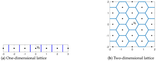
Figure 2.
Examples of one- and two-dimensional lattices with generator matrices and , respectively. The lattice points are marked by black crosses, whereas the Voronoi cell partitions are marked by blue lines.
Definition 2
(Nearest-neighbor quantizer and Voronoi cell [15] (Chapter 2.2)). The nearest-neighbor quantizer induced by a k-dimensional lattice Λ is defined as
The Voronoi cell is the set of all points that are quantized to :
is referred to as the fundamental Voronoi cell. The breaking of ties in (16) is carried out in a systematic manner so that the induced Voronoi cells are congruent. In particular,
- for , where the first sum is the Minkowski sum of and the singleton ;
- for , where ;
- .
We next define the modulo-lattice operation with respect to the fundamental Voronoi cell.
Definition 3
(Modulo-lattice [15] (Chapter 2.3)). For a k-dimensional lattice Λ with a fundamental Voronoi cell , the modulo-lattice operation (with respect to ), applied to , is defined as
namely, the outcome equals the (unique) point that satisfies for some .
We now define the volume, the second moment, and the normalized second moment of a lattice.
Definition 4
(Volume and second moment [15] (Chapter 2 and 3)). The volume of a k-dimensional lattice Λ with fundamental Voronoi cell is defined as the volume of :
The second moment of Λ is defined as the second moment per dimension of a random variable that is uniformly distributed over :
The normalized second moment of Λ is defined as
To attain a good MMSE using lattice quantization, should be as close as possible to the normalized second moment of a k-dimensional ball which, in the limit of , converges to .
Since the effective source in intermediate layers (this will become clear in the following section) that we would like to transmit and the effective channel noise which is induced by the analog modulations over the continuous-time channel are not Gaussian in general (even after “Gaussianization” which would make them only approximately so), we would need to consider more general source and channel noise vectors that satisfy the following definition of semi-norm ergodicity (SNE).
Definition 5
(SNE [22] (Def. 2)). A sequence in k of random vectors of length k with a limit norm . (The original definition of [22] (Def. 2) requires for all . We use here a more relaxed definition which will prove more convenient in the following section):
is SNE if for any , however small, there exists a large enough , such that for all
We are now ready to describe the k-dimensional JSCC setting and the MLM technique with side information (SI) for this setting. In the overall solution of Section 5, the analog modulations over the continuous-time channel that will be described in Section 4 will translate the channel into an effective k-dimensional additive SNE noise channel (compare also the subfigures of Figure 4 in Section 5. Over this effective channel, MLM with SI will be employed, where we will treat previous source estimators as effective side information (SI) known to the receiver but not to the transmitter [13] and [15] (Chapter 11).
Source. Consider a source sequence (equivalently, vector) of length k,
where is an SI sequence which is known to the receiver but not to the transmitter, and is the “unknown part” (at the receiver) with per-element variance
and is SNE (as a sequence in k).
Transmitter. Maps to a channel input, , that is subject to a power constraint
Channel. The channel is an additive noise channel:
where is an SNE noise vector that is uncorrelated with and has effective variance
The SNR is defined as ; we use here the more common SNR notion in lieu of the ENR notion to emphasize that the channel and the source vectors (equivalently, sequences) in this section are of the same dimension k, in contrast to the continuous-time channel of Section 2.
Receiver. Receives , in addition to the SI , and generates an estimate of the source .
The following MLM-based scheme will be employed in the following.
- Scheme 1. [MLM-based JSCC with SI [13], [15] (Chapter 11)]
Transmitter: Transmits the signal
where is a lattice with a fundamental Voronoi cell and a second moment P, is a scalar scale factor, and is a dither vector which is uniformly distributed over and is independent of the source vector ; consequently, is independent of by the so-called crypto lemma [15] (Chapter 4.1).
Receiver:
- Receives the signal (27) and generates the signalwhere is the equivalent channel noise, and is a channel scale factor.
- Generates an estimate :where is a source scale factor.
When in (30) falls within , the modulo operation does not come into play, resulting in an effective additive noise channel from to . Thus, we want the probability of this “correct lattice decoding” event to be bounded from below by for some small . On the other hand, conditioned on the correct lattice decoding event, we want the quantization noise, which is governed by , and consequently by the shape of , to have a small normalized second moment to be good for MMSE estimation. The following theorem provides guarantees for the achievable distortion using this scheme and is aggregated from [13], [15] (Chs. 11.3, 6.4, 9.3), and [22] (see also the exposition about correlation-unbiased estimators (CUBEs) in [23]).
Theorem 1.
The distortion (10) of Scheme 1 is bounded from above by
for , and that satisfy
where
is the distortion given a lattice-decoding-error event [13] (Equation (24)) and is bounded from above by
and the lattice parameters and are defined as
Moreover, for any , however small, and any , there exists a sequence of lattices, , that are good for both channel coding [22] (Def. 4) and mean squared error (MSE) quantization [22] (Def. 5), viz.,
respectively, and, therefore, this sequence of lattices achieves a distortion that approaches .
Remark 1.
By our definition of SNE sequences, for each finite k the actual variance of the unknown part and the noise variance may be higher than for every higher than their asymptotic quantities. Consequently, also the second moment of for every would be taken to be higher than its asymptotic value.
The following choice of parameters is optimal in the limit of infinite blocklength, , in the Gaussian case ( comprises i.i.d. Gaussian samples, comprises i.i.d. Gaussian samples) [4] (Chapter 11.3) when the SNR is known.
Corollary 1
(Optimal parameters [13], [15] (Chapter 11.3)). The choice , , , , yields a distortion D that is bounded from above as in (32) with
where
Moreover, for any , however small, there exists a sequence of lattices that attains (38) and, therefore, in the limit , and above converge to and the distortion D approaches , which converges, in turn, to
Consider now the setting of an SNR that is unknown at the transmitter but is known at the receiver. In this case, although the receiver knows the SNR and can, therefore, optimize and accordingly, the transmitter, being oblivious of the SNR, cannot optimize for the true value of the SNR. Instead, by setting in accordance with Corollary 1 for a preset minimal-allowable-design SNR, , Scheme 1 achieves (44) for and improves, albeit sublinearly, with the SNR for . This is detailed in the next corollary.
Corollary 2
(SNR universality). Assume that for some predefined . Then, the choice , , and with respect to (as it cannot depend on the true SNR), and and (may depend on the true SNR) yields a distortion D that is bounded from above, as in (32) for that is given in (39) with . Moreover, for any , however small, there exists a sequence of lattices that satisfies (38); therefore, in the limit , converges to , converges to , and the distortion D approaches , which converges, in turn, to
Corollary 3
(Source power uncertainty). Assume now additionally that the transmitter is oblivious of the exact power of , , but knows that it is bounded from above by : . Then, the distortion is bounded according to (32), with
for the parameters
Moreover, for any , however small, there exists a sequence of lattices that attains (38) and, therefore, in the limit of , converges to , converges to , and the distortion D is bounded from above in this limit by :
where ϵ decays to zero with . For , the bound (48c) approaches .
The following result is a simple consequence of Theorem 1 and avoids exact computation of the optimal parameters.
Corollary 4
(Suboptimal parameters). Assume the setting of Corollary 3 but with not necessarily uncorrelated with , and denote . Then, the distortion is bounded according to (32) with
for the parameters , .
We refer to by since now may depend on .
The following property will prove useful in Section 5 when treating non-Gaussian noise through “Gaussianization”.
Lemma 1
([24] (Lemmas 6 and 11)). Let be a sequence of lattices that satisfies the results in this section, and let be a dither that is uniformly distributed over the fundamental Voronoi cell of . Then, the probability density function (p.d.f.) of is bounded from above as
where is the p.d.f. of a vector with i.i.d. Gaussian entries with zero mean and the same second moment P as , and decays to zero with k.
4. Background: Analog Modulations in the Known-ENR Regime
Following the exposition at the beginning of Section 3 and Figure 3, we concentrate now on the second major component that is used in this work, that of analog modulations for conveying a scalar zero-mean Gaussian source () over a channel with infinite bandwidth, where both the receiver and the transmitter know the channel noise level, or equivalently, . To that end, we will review next the analog linear modulation and the analog PPM and will supplement the known results for the latter with a new robustness result for a source distribution that deviates from Gaussianity in Corollary 6.
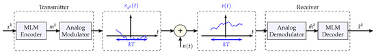
Figure 3.
High-level description of the JSCC scheme (Scheme 2). Our construction consists of a concatenation of an MLM encoder and an analog modulation that maps the encoded signals into a continuous-time waveform. On the receiver, we apply the inverse operations by first demodulating the analog signal and then use an MLM decoder.
Consider first analog linear modulation, in which the source sample x is linearly transmitted with energy E, (under linear transmission, the energy constraint holds only on average, and the transmitted energy is equal to the square of the specific realization of x) using some unit-energy waveform
Note that linear modulation is the same (“universal”) regardless of the true noise level. Signal space theory [25] (Chapter 8.1), [26] (Chapter 2) suggests that a sufficient statistic of the transmission of (51) over the channel (9) is the one-dimensional projection y of r onto :
where z is a standard Gaussian noise variable. The MMSE estimator of x from y is linear and its distortion is equal to
and improves only linearly with the .
Consider now analog PPM, in which the source sample is modulated by the shift of a given pulse rather than by its amplitude (which is the case for analog linear modulation):
where is a predefined pulse with unit energy and is a scaling parameter. In particular, the square pulse (Clearly, the bandwidth of this pulse is infinite. By taking a large enough bandwidth W, one may approximate this pulse to an arbitrarily high precision and attain its performance within an arbitrarily small gap) is known to achieve good performance. This pulse is given by
for a parameter , which is sometimes referred to as effective dimensionality. Clearly, .
The optimal receiver is the MMSE estimator of x given the entire output signal:
The following theorem provides an upper bound on the achievable distortion of this scheme using (suboptimal) maximum a posteriori (MAP) decoding, which is given by
where
is the (empirical) cross-correlation function between r and with lag (displacement) , and
is the autocorrelation function of with lag .
Remark 2.
Since a Gaussian source has infinite support, the required overall transmission time T is infinite. Of course, this is not possible in practice. Instead, one may limit the transmission time T to a very large—yet finite—value. This will incur a loss compared to the the bound that will be stated next; this loss can be made arbitrarily small by taking T to be large enough.
Theorem 2
([21] (Prop. 2)). The distortion of the MAP decoder (57) of a standard Gaussian scalar source transmitted using analog PPM with a rectangular pulse is bounded from above by
with
bounding the small- and large-error distortions, assuming . In particular, in the limit of large , and β that increases monotonically with ,
where
and in the limit of .
Remark 3.
For a fixed β, the distortion improves quadratically with the . This behavior will prove useful in the next section, where we construct schemes for the unknown-ENR regime.
Setting in (60) of Theorem 2 yields the following asymptotic performance.
Corollary 5
([21] (Th. 2)). The achievable distortion of a standard Gaussian scalar source transmitted over an energy-limited channel with a known ENR is bounded from above as
where as .
The following corollary, whose proof is available in Appendix A, states that the (bound on the) distortion is continuous in the source p.d.f. around a Gaussian p.d.f. Such continuity results of the MMSE estimator in the source p.d.f. are known [27]. Next, we prove the required continuity directly for our case of interest with an additional technical requirement on the deviation from a Gaussian p.d.f.; this result will be used in conjunction with a non-uniform variant of the Berry–Esseen theorem in Section 5.
Corollary 6.
Consider the setting of Theorem 2 for a source p.d.f. that satisfies
where , is the standard Gaussian p.d.f., and is a symmetric absolutely continuous non-negative bounded function with unit integral , that is monotonically decreasing for (and for , by symmetry) and satisfies ; thus, there exists such that
Then, the distortion of the decoder that applies the decoding rule (57) is bounded from above by
where denotes the bound on the distortion for a standard Gaussian source of Theorem 2, and is a non-negative constant that depends on . (This is no longer the MAP decoding rule since is no longer a Gaussian p.d.f.).
5. Main Results
In this section, we construct JSCC solutions for the unknown-ENR communication problem. As already explained at the beginning of Section 3, the proposed solution, which is depicted in Figure 3 (cf. Figure 1), is composed of two major components:
- Aa layered MLM-based component that works well for a continuum of possible noise levels over k-dimensional additive SNE noise channels, where each layer accommodates a different noise level, with layers of lower noise levels acting as SI in the decoding of subsequent layers;
- An analog modulation component that is designed for a particular ENR of the continuous-time channel but improves for high ENRs and induces a k-dimensional additive SNE noise channel for the first component.
Following the exposition in the introduction, since an exponential improvement with the ENR cannot be attained in this setting for an infinite number of noise levels let alone a continuum thereof [7], following [7,18], we consider polynomially decaying profiles (6a,b).
We first show, in Section 5.1, that replacing the successive refinement coding of [7,18] with MLM (Wyner–Ziv coding) with linear layers results in better performance in the infinite-bandwidth setting (paralleling the results of the bandwidth-limited setting [6]).
In Section 5.2, we replace the last layer with an analog PPM one, which improves quadratically with the ENR ( in (6b)) above the design ENR (recall Remark 3).
In principle, despite analog PPM attaining a gracious quadratic decay with the ENR (recall Remark 3) only above a predefined design ENR, since the distortion is bounded from above by the (finite) variance of the source, it attains a quadratic decay with the ENR for all , or equivalently, for all and in (6a,b).
That said, the performance of analog PPM deteriorates rapidly when the ENR is below the design ENR of the scheme, meaning that the minimum energy required to obtain (6a) with and a given is large. To alleviate this, we use the above-mentioned layered MLM scheme. Furthermore, to achieve higher-order improvement with the ENR ( in (6a,b)), multiple layers in the MLM scheme need to be employed.
We now present a simplified variant of the general scheme that is considered throughout this section. This variant is also depicted in Figure 4a. The full scheme, which incorporates interleaving for analytical purposes, is available in Appendix B and depicted in Figure A1.
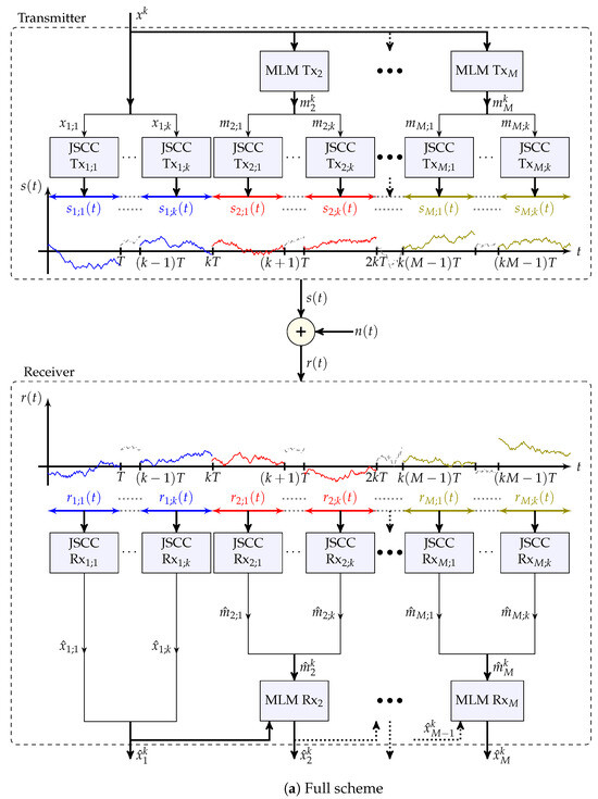
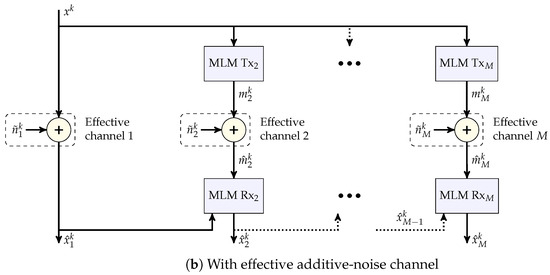
Figure 4.
Block diagrams of Scheme 2 and of this scheme with the effective additive noise channels of Remark 6.
- Scheme 2 (MLM-based).
M-Layer Transmitter:
First layer ():
Other layers: For each :
- Calculates the k-dimensional tuplewhere , and denotes the entry of ; , , and take the roles of the , and of Scheme 1, and are tailored for each layer i; is chosen to have unit second moment.
- For each , views as a scalar-source sample, and generates a corresponding channel input,using a scalar JSCC scheme with a predefined energy that is designed for a predetermined , or equivalently, , such that and .
First layer (): For each :
- Recovers the MMSE estimate of given , where .
- If the true noise level N satisfies , sets the final estimate of to and stops. Otherwise, determines the maximal layer index for which and continues to process the other layers.
Other layers: For each in ascending order:
- For each , uses the receiver of the scalar JSCC scheme to generate an estimate of from , where
- Using the effective channel output (that takes the role of in Scheme 1) with SI , generates the signalas in (30) of Scheme 1, where is a channel scale factor.
- Constructs an estimate of :as in (31) of Scheme 1, where is a source scale factor. The final estimate if .
Remark 4
(Interleaving). To guarantee independence between all the noise entries , we use interleaving in the full scheme, which is described in Appendix B in (A8) and (A11). We note that this operation is used to simplify the proof that the resulting noise vector is SNE (recall Definition 5).
Remark 5
(Gaussianization). To use the analysis of Section 4 of analog PPM for a Gaussian source, we multiply the vectors by orthogonal matrices that effectively “Gaussianize” its entries, as shown in the full description of the scheme in Appendix B, in (A8) and (A11). In particular, this is achieved by a Walsh–Hadamard matrix by appealing to the central limit theorem; a similar choice was previously proposed by Feder and Ingber [28], and by Hadad and Erez [29], where in the latter, the columns of the Walsh–Hadamard matrix were further multiplied by i.i.d. Rademacher RVs to achieve near-independence between multiple descriptions of the same source vector (see [29,30,31] for other ensembles of orthogonal matrices that achieve a similar result). Interestingly, the multiplication by the orthogonal matrices (since Walsh–Hadamard matrices are symmetric, they further satisfy ) Gaussianizes the effective noise incurred at the outputs of the analog PPM JSCC receivers.
Remark 6
(JSCC-induced channel). The continuous-time JSCC transmitter and receiver over the infinite-bandwidth AWGN channel induce an effective additive-noise channel of better effective SNR and source bandwidth. Over this induced channel, the MLM transmitter and receiver are then employed. This interpretation is depicted in Figure 4b, with representing the effective additive noise vectors.
We next provide analytic guarantees for this scheme for linear and analog PPM layers in Section 5.1 and Section 5.2, respectively, in the infinite-blocklength regime. In Section 6, we compare the analytic and empirical performance of these schemes in the infinite-blocklength regime, as well as comparing the empirical performance of these schemes for a single-source sample. The treatment of the infinite-blocklength regime pertains to the full scheme as presented in Appendix B. The comparison for a single-source sample, uses the simplified variant of Scheme 2.
5.1. Infinite-Blocklength Setting with Linear Layers
We start with analyzing the performance of the scheme where all the M layers are transmitted linearly and M is large; we concentrate on the setting of an infinite-source blocklength () and derive an achievability bound on the minimum energy that achieves a polynomial distortion profile (6a,b). A constructive proof of the next theorem is available in Appendix C. In particular, this proof specifies all the scheme parameters, such as the energy allocated to each layer and the minimal noise level it is designed for.
Theorem 3.
Choose a decaying order , a design parameter , and a minimal noise level , however small. Then, a distortion profile (6a) with L and is achievable for all noise levels for any transmit energy E that satisfies
for a large-enough-source blocklength k, where
In particular, the choice achieves a quadratic decay () for any transmit energy E that satisfies
for a large-enough-source blocklength k.
We note that already this variant of the scheme offers an improvement compared to the hitherto best-known upper (achievability) bound of (7).
The choice of the minimal noise level dictates the number of layers M that need to be employed: the lower is, the more layers M need to be employed.
Remark 7.
In the proof in Appendix C, we use an exponentially decaying noise level series , which facilitates the analysis. Nevertheless, any other assignment that satisfies the profile requirement and energy constraint is valid and may lead to better performance; for further discussion, see Section 7.
5.2. Infinite-Blocklength Setting with Analog PPM Layers
In this section, we concentrate on the setting of an infinite-source blocklength () and a quadratically decaying profile ( in (6a,b)) using analog PPM.
To that end, we use a sequence of linear JSCC layers as in Section 5.1, with only the last layer replaced by an analog PPM one; since analog PPM improves quadratically with the ENR (recall Remark 3), M need not go to infinity to attain a quadratically decaying profile.
Theorem 4.
Choose a design parameter , and a minimal noise level , however small. Then, a quadratic profile () (6a) with is achievable for all noise levels for any transmit energy E that satisfies
for a large-enough-source blocklength k.
This theorem, whose proof is available in Appendix D, offers a further improvement over the upper bounds in (7) and Theorem 3 for a quadratic profile. Again, the proof of Theorem 4 in Appendix D is constructive and details the scheme parameters, such as the energy allocated to each layer and the minimal noise level, it is designed for.
Remark 8.
Replacing all layers but the first layer with analog PPM ones should yield better performance, but complicates the analysis. Moreover, a similar analysis to that of Theorem 3 for may be devised, but for would require multiple layers as the distortion of analog PPM decays only quadratically. Both of these analyses are left for future research.
6. Simulations
In Section 6.1, we first compare the analytical results of Theorems 3 and 4 to the prior art in the infinite-blocklength regime (). We further optimize the parameters in Theorem 4 empirically and show a further improvement, which suggests, in turn, a slack in our analysis. In Section 6.2, we evaluate the performance of Scheme 2 empirically, using a Monte Carlo simulation, for a single-source sample () of a uniform source, and compare the performance of a scheme with all linear layers to those of a scheme that incorporates an analog PPM layer.
6.1. Analytical Performance Comparison in the Infinite-Blocklength Regime
We first consider the infinite-blocklength regime () for a Gaussian source and a quadratic profile ( in (6a,b)), for which we have derived analytical guarantees in Section 5.1 and Section 5.2. Figure 5 depicts the accumulated energy of the employed layers at the receiver of Section 5 and the achievable distortion as functions of , along with the desired quadratic distortion profile (6a) (with ) for for linear layers with the energy allocation to the different layers, as per the proof of Theorem 3 in Appendix C; and linear layers with a final analog PPM layer (Theorem 4) for both the energy allocation for layers, which is available in the proof of Theorem 4 in Appendix D and relies on the bound on the analog PPM performance, and for layers, with an empirically evaluated performance of analog PPM allocation.
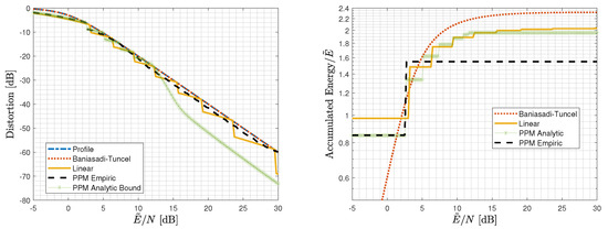
Figure 5.
Distortion and accumulated energy of the layers utilized by the receiver at a given for a Gaussian source in the infinite-blocklength regime for a quadratic profile: Scheme 2 with linear layers with energy allocation for and . Empirical performance of the scheme with a linear layer with energy and an analog PPM layer with energy , and analytic performance of the scheme of Theorem 4 with the parameters from its proof, and analytic performance of the scheme of Baniasadi and Tuncel [18].
This figure clearly demonstrates the gain due to introducing an analog PPM layer. Interestingly, the empirically evaluated analog PPM curve shows that only two layers are needed when the second layer is an analog PPM one, meaning that the seven layers needed in the proof of Theorem 4 are an artifact of the slack in our analytic bounds.
To derive the performance of the scheme with linear layers, we evaluated the energy allocation in the proof of Theorem 3 in Appendix C in (16) directly for the optimized energy allocation with and . To derive the analytical performance of Theorem 4, we used the energy allocation from its proof in Appendix D, while for the empirical performance, optimizing over the energy allocation yielded . The Matlab code package and the specific script that was used for generating Figure 5, along with all the scheme parameters and analog PPM empirical evaluation, are available in [32].
6.2. Empirical Performance Comparison for a Single-Source Sample
We move now to the uniform scalar-source setting () and a quadratic profile. The analysis of Section 5 in the scalar setting is difficult. We, therefore, evaluate its performance empirically for both variants of the scheme: with linear layers, and with one linear layer and one analog PPM layer (two layers suffice in this setting as well). In Figure 6, we depict again the accumulated energy of the employed layers at the receiver of Section 5 and the achievable distortion as functions of for both variants of the scheme, along with the desired quadratic distortion profile (6a) (with ) for .
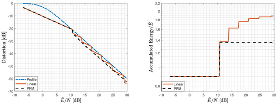
Figure 6.
Distortion and accumulated energy of the layers utilized by the receiver at a given for a uniform scalar source for a quadratic profile: Scheme 2 with linear layers with energy allocation for and , and with a linear layer with energy and an analog PPM layer with energy . The value was optimized according to (76).
For the variant with linear layers only, an energy allocation of with and was used. For the variant with an analog PPM layer, an energy of was allocated to the (first) linear layer, and an energy of was allocated to the (second) analog PPM layer. The lattice inflation factor was chosen as the minimizer of a variant of (32) under the assumption that the noise is Gaussian, namely,
where , N is the noise level, is the modulo size that was chosen to be , and is the average distortion that corresponds to the last transmitted layer.
As in the infinite-blocklength regime, here too utilizing analog PPM provides better performance compared to a linear-only scheme. Again, the Matlab code package and the specific script that was used for generating Figure 6, along with all the scheme parameters and empirical evaluations, are available in [32].
7. Summary and Discussion
In this work, we studied the problem of JSCC over an energy-limited channel with unlimited bandwidth and/or transmission time when the noise level is unknown at the transmitter. We showed that MLM-based schemes outperform the existing schemes thanks to the improvement in the performance of all layers (including the preceding layers that act as SI) with the ENR. By replacing (some of the) linear layers with analog PPM ones, further improvement was achieved. We further demonstrated numerically that the MLM-layered scheme works well in the scalar-source regime.
We also note that a substantial gap remains between the lower bound in (7) and the upper bound of Theorem 4 for the energy required to achieve a quadratic profile ((6a,b) with ). In Section 8, several ways to close this gap are described.
We note that, although we assumed that both the bandwidth and the time are unlimited, the scheme and analysis presented in this work carry over to the setting where one of the two is bounded as long as the other one is unlimited, with little adjustment.
8. Future Research
Consider first the remaining gap between the lower and upper bounds. As demonstrated in Section 6, the upper (achievability) bound on the performance of analog PPM is not tight and calls for further improvement thereof. This step is currently under intense investigation, along with improvement via companding of the presented analog PPM variant in this work as well as via other choices of energy allocation (see Remark 7). Furthermore, the optimization was performed numerically and for a particular form of noise levels of an exponential form (recall Remark 7). We believe that a systematic optimization procedure could shed light on the weaknesses of our scheme and provide further improvements in the overall performance. On the other hand, the outer bounds of [18] are based on specific choices of sequences of noise levels. Therefore, further improvement might be achieved by other choices and calls for further research.
We have also shown that the MLM scheme performs well in the scalar-source regime; it would be interesting to derive analytical performance guarantees for this regime.
Finally, since MLM utilizes well source SI at the receiver and channel SI at the transmitter [13,14], [15] (Chs. 10–12), the proposed scheme can be extended to limited-energy settings, such as universal transmission with respect to the noise level and the SI quality at the receiver [33] and the dual problem of the one considered in this work of universal transmission with respect to the noise level with near-zero bandwidth [34].
Author Contributions
Writing—original draft, O.L. and A.K. All authors have read and agreed to the published version of the manuscript.
Funding
This work was supported by the Israel Science Foundation (grant No. 2077/20). The work of O. Lev was further supported by the Yitzhak and Chaya Weinstein Research Institute for Signal Processing. The work of A. Khina was further supported by the WIN Consortium through the Israel Ministry of Economy and Industry, and by a grant from the Tel Aviv University Center for AI and Data Science (TAD).
Institutional Review Board Statement
Not applicable.
Data Availability Statement
Not applicable.
Conflicts of Interest
The authors declare no conflict of interest.
Appendix A. Proof of Corollary 6
To prove Corollary 6, we repeat the steps of the proof of Theorem 2 in [21] (Prop. 2); we next detail the contributions to the small-distortion [21] (Equation (25)) and the large-distortion [21] (Equation (27)) terms due to the deviation (64) from the source p.d.f. from Gaussianity, which are denoted by and , respectively.
We start by bounding the contribution to the small-distortion term. To that end, note that [21] (Equations (24b) and (25b)) remain unaltered since the decoder remains the same. The contribution to the small-distortion term is bounded from above as follows.
where (A1a) follows from [21] (Equations (24b) and (25b)), and (A1b) follows from being non-negative with unit integral.
We next bound the contribution to the large distortion term. To that end, note that [21] (Equations (27) and (28)) remain unaltered since the decoder remains the same. We define by the deviation in in [21] (Equation (30)). Then,
where (A2a) follows from [21] (Equations (28) and (30)), (A2b) follows from integration by substitution and (65), and (A2c) follows from (65) for some .
Appendix B. Full Version of Scheme 2
We now present the full multi-layer transmission scheme (cf. Scheme 2), which includes interleaving and Gaussianization steps, as discussed in Remarks 4 and 5, respectively. Block diagrams of the overall scheme and the new ingredients are provided in Figure A1 and Figure A2, respectively. The new components in Scheme 3 compared to those in Scheme 2 (and Figure 4a) are highlighted in green in Figure A1.

Figure A1.
Block diagram of Scheme 3.
Figure A1.
Block diagram of Scheme 3.


Figure A2.
Block diagram for the i-th MLM layer transmitter and receiver of Scheme 3. We denote the interleaving and de-interleaving operations by and , respectively.
Figure A2.
Block diagram for the i-th MLM layer transmitter and receiver of Scheme 3. We denote the interleaving and de-interleaving operations by and , respectively.

- Scheme 3 (Full MLM-based).M-Layer Transmitter:
First layer ():
- For , , accumulates source (column) vectors . Denote by the matrix whose columns are the source vectors:
Other layers: For each :
- For each , calculates the k-dimensional tuplewhere , and denotes the entry of for ; , , and take the roles of , and of Scheme 1, and are tailored for each layer i; is chosen to have unit second moment.
- For each , interleaves the entries , stacks them into vectors of size B, and applies to each of them a B-dimensional orthogonal matrix , as follows:for , where is the vector after interleaving; is the vector after interleaving and matrix multiplication and its entry is for ; the length of the vectors and is B. Note that the interleaving operation creates doubly indexed vectors, where a set of vectors of length k is transformed into vectors of length B, which are indexed by and .
- For each ℓ, j, and , views as a scalar-source sample, and generates a corresponding channel input , whereusing a scalar JSCC scheme with a predefined energy that is designed for a predetermined , or equivalently, , such that and .
First layer (): For each , :
- Recovers the MMSE estimate of given , whereDenotes the matrix whose columns comprise these estimates by
- If the true noise level N satisfies , sets the final estimate of to and stops. Otherwise, determines the maximal layer index 𝚥 for which and continues to process the other layers.
Other layers: For each in ascending order:
- For each and , uses the receiver of the scalar JSCC scheme to generate an estimate of from , where
- For each , stacks the entries of into vectors of length B, , applies the orthogonal matrix to each vector , and de-interleaves the outcomes, to attain , as follows:for .
- For each , using the effective channel output (that takes the role of in Scheme 1) with SI , generates the signalas in (30) of Scheme 1, where is a channel scale factor.
- For each , constructs an estimate of :as in (31) of Scheme 1, where is a source scale factor. Denote the matrix whose columns comprise these estimates by . The final estimate is .
Appendix C. Proof of Theorem 3
To prove Theorem 3, we will make use of the following lemma about the validity of the MLM results from Section 3 for the multi-layer MLM scenario, where the mid-stage noise vectors are linear combinations of dithers and Gaussian noises. The proof of this lemma is given in Appendix E.
Lemma A1.
Let be a sequence in k of vectors, such that the vector equals with probability to a linear combination of a Gaussian vector and dithers, all of which are mutually independent, where . Then, the sequence in k of error signals is SNE for a sequence of lattices that is good for both channel coding and MSE quantization; moreover, for each k, the error signal is equal, with probability , to a linear combination of a Gaussian vector and dithers, all of which are mutually independent, where .
We now prove Theorem 3. We will construct a scheme with a large enough (yet finite) M that achieves (6a) with the predefined L and for all for a given . For any , however small, we will choose large enough and such that .
Consider the first layer (). The distortion of for a noise level N is bounded from above by
where (A14a) follows from (53), and (A14b) and (A14c) follow from the distortion profile requirement (6a) for .
To guarantee the requirement (A14b) for all , it suffices to guarantee it for the extreme value , which holds, in turn, for
For , the distortion of for a noise level N is bounded from above by
where (A16a) follows from Corollary 2 by treating as SI, and the error takes the role of the “unknown part” at the receiver with power , with going to zero with k, and by invoking Lemma A1 recursively, which guarantees that the sequence in k of the error vectors is SNE; (A16b) holds by the distortion profile requirement (6a) (the requirement is satisfied for for any , however small, and therefore, holds also for , by continuity. Alternatively, one may view it as a requirement of the scheme given layers, for all ); (A16c) follows from (6a) with and L; (A16d) follows from the distortion profile requirement (6a) for ; and (A16e) follows from (6a) with and L.
To guarantee the requirement (A16d) for all we need only to satisfy it for the extreme value , which holds, in turn, for
where (A17b) holds since , and decays to zero with k; the set of inequalities (A17a,b) holds for
where again decays to zero with k.
We are now ready to bound the total energy E.
where (A19b) follows from (A15) and (A18), in (A19c) we use the choice for the noise levels for some positive parameters and , and (A19d) holds by defining .
Finally, by optimizing over the parameters and x, taking a large enough M, and taking k to infinity, we arrive at the desired result.
Appendix D. Proof of Theorem 4
To prove Theorem 4, we will make use of the following non-uniform variant of the Berry–Esseen theorem, which is a weakened (yet more compact) form of a result due to Petrov.
Theorem A1
([35] and [36] (Chapter VII, Thm. 17)). Let be an i.i.d. sequence of RVs with zero mean and unit variance, and denote . Assume that for some , and that has a bounded p.d.f. Then, the p.d.f. of , denoted by , satisfies
for some , where is the standard Gaussian p.d.f.
Furthermore, as discussed in Remarks 4–6, in each layer (and specifically in the PPM layer) we effectively have an additive noisy channel whose noise distribution approaches a Gaussian distribution (due to the Gaussianization and the interleaving). For all the linear layers, Lemma A1 allows us to use the MLM results of Section 3. However, for the PPM layer, instead of a combination of Gaussian vectors and dithers (as treated in Lemma A1) the actual noise also contains terms that are induced by the PPM scheme. We will use the following lemma, which is proved in Appendix F, to claim that the effect of these terms on the performance of the MLM scheme can be made arbitrarily small by taking the dimension k to be large enough.
Lemma A2.
Let be a sequence in k of SNE vectors with second moment such that , and let be a corresponding sequence in k of vectors with identically distributed entries such that:
- The distance between the p.d.f. of and that of is bounded from above bywhere with meaning that , and where and denote the first entries of the vectors and , respectively.
- The correlation between any two squared entries within decays to zero with k, viz..,where denotes the covariance of A and B.
Then, for all , there exists such that
for all , namely, the sequence is a sequence of SNE vectors.
We will now prove Theorem 4. We note that the following analysis is based on the interleaving and Gaussianization blocks as they appear in the full description of the scheme in Appendix B.
Proof of Theorem 4.
We will now derive the parameters that achieve a quadratic profile () and in (6a) for all for a given .
We choose for the linear layers—layers . Consequently, the analysis for the first layers of the proof of Theorem 3 carries over to this scheme as well.
Consider now the last layer—layer M. Following Feder and Ingber [28], and Hadad and Erez [29], we use a B-dimensional Walsh–Hadamard matrix .
Now, if , the receiver uses the last layer to improve the source estimates while viewing the estimates resulting from the previous layer, , as SI with mean power (A16a–e).
By Lemma 1, all the moments of all the entries of exist and are finite for all b. Thus, by Theorem A1, and since are i.i.d., the p.d.f. of (it is the same for all b and j for a given ℓ) satisfies
for all , , and , for all for some , where is the p.d.f. of a zero-mean Gaussian RV with the same variance as .
By choosing some and applying Corollary 6 to with and , the distortion bound of Theorem 2 is attained up to a loss for some constant , where this loss can be made arbitrarily small by choosing a large enough B.
We note that the interleaving makes the PPM transmitters operate over elements that are related to lattices of different sources. Thus, after de-interleaving, the correlation between different vector elements, as well as the correlation between their squares, vanishes as . Furthermore, the per-element variance is bounded from above by a quantity that approaches (as ) the PPM performance bound of Theorem 2. Thus, by Lemma A2, the resulting effective noise vector is SNE (recall Definition 5).
We note that is correlated with ; nevertheless, by Corollary 4 with parameters the distortion of is bounded from above by
where subsumes the aforementioned losses that all go to zero with k, and is the SDR of the analog PPM scheme for a noise power N of Theorem 2.
The energy of the last layer is chosen to comply with the profile for :
Combining (A25) and the contribution of the first layers, given by (A19c) with summation from 1 to , by numerically optimizing the resulting term over the number of layers M, the PPM pulse width and the energy layers we obtain that , , and the layer energies , , , yields (75). □
Appendix E. Proof of Lemma A1
Since is assumed to be a sequence that is good for channel coding,
where ; equivalently, for any , however small, there exists , such that for all ,
Note now that equals a linear combination of independent Gaussian vectors—which amounts to a Gaussian vector—and dither vectors. Hence, by [22] (Th. 3), the sequence in k of vectors is SNE, namely, for any , however small, there exists , such that for all ,
Now, let , however small and choose , and . Then, by the union bound, for all ,
References
- Cover, T.M.; Thomas, J.A. Elements of Information Theory, 2nd ed.; Wiley: New York, NY, USA, 2006. [Google Scholar]
- Köken, E.; Gündüz, D.; Tuncel, E. Energy–Distortion Exponents in Lossy Transmission of Gaussian Sources Over Gaussian Channels. IEEE Trans. Inf. Theory 2016, 63, 1227–1236. [Google Scholar] [CrossRef]
- Sevinç, C.; Tuncel, E. On Asymptotic Analysis of Energy–Distortion Tradeoff for Low-Delay Transmission over Gaussian Channels. IEEE Trans. Commun. 2021, 69, 4448–4460. [Google Scholar] [CrossRef]
- El Gamal, A.; Kim, Y.H. Network Information Theory; Cambridge University Press: Cambridge, UK, 2011. [Google Scholar]
- Shannon, C.E. Coding Theorems for a Discrete Source With a Fidelity Criterion of the Institute of Radio Engineers, International Convention Record; Wiley: New York, NY, USA, 1959; Volune 7, pp. 142–163. [Google Scholar]
- Reznic, Z.; Feder, M.; Zamir, R. Distortion bounds for broadcasting with bandwidth expansion. IEEE Trans. Inf. Theory 2006, 52, 3778–3788. [Google Scholar] [CrossRef]
- Köken, E.; Tuncel, E. On minimum energy for robust Gaussian joint source–channel coding with a distortion–noise profile. In Proceedings of the IEEE International Symposium on Information Theory (ISIT), Aachen, Germany, 25–30 June 2017; pp. 1668–1672. [Google Scholar]
- Equitz, W.H.R.; Cover, T.M. Successive Refinement of Information. IEEE Trans. Inf. Theory 1991, 37, 851–857. [Google Scholar] [CrossRef]
- Santhi, N.; Vardy, A. Analog codes on graphs. In Proceedings of the IEEE International Symposium on Information Theory (ISIT), Yokohama, Japan, 29 June–5 July 2003; p. 13. [Google Scholar]
- Santhi, N.; Vardy, A. Analog codes on graphs. arXiv 2006, arXiv:cs/0608086. [Google Scholar]
- Bhattad, K.; Narayanan, K.R. A note on the rate of decay of mean-squared error with SNR for the AWGN channel. IEEE Trans. Inf. Theory 2010, 56, 332–335. [Google Scholar] [CrossRef]
- Mittal, U.; Phamdo, N. Hybrid digital-analog (HDA) joint source–channel codes for broadcasting and robust communications. IEEE Trans. Inf. Theory May 2002, 48, 1082–1102. [Google Scholar] [CrossRef]
- Kochman, Y.; Zamir, R. Joint Wyner–Ziv/Dirty-Paper Coding by Modulo-Lattice Modulation. IEEE Trans. Inf. Theory 2009, 55, 4878–4899. [Google Scholar] [CrossRef]
- Kochman, Y.; Zamir, R. Analog matching of colored sources to colored channels. IEEE Trans. Inf. Theory 2011, 57, 3180–3195. [Google Scholar] [CrossRef]
- Zamir, R. Lattice Coding for Signals and Networks; Cambridge University Press: Cambridge, UK, 2014. [Google Scholar]
- Wyner, A.D.; Ziv, J. The Rate–Distortion Function for Source Coding with Side Information at the Decoder. IEEE Trans. Inf. Theory 1976, 22, 1–10. [Google Scholar] [CrossRef]
- Wyner, A.D. The Rate–Distortion Function for Source Coding with Side Information at the Decoder—II: General Sources. Inf. Control 1978, 38, 60–80. [Google Scholar] [CrossRef]
- Baniasadi, M.; Tuncel, E. Minimum Energy Analysis for Robust Gaussian Joint Source–Channel Coding with a Square-Law Profile. In Proceedings of the IEEE International Symposium on Information Theory and Its Applications (ISITA), Kapolei, HI, USA, 24–27 October 2020; pp. 51–55. [Google Scholar]
- Baniasadi, M.; Köken, E.; Tuncel, E. Minimum Energy Analysis for Robust Gaussian Joint Source–Channel Coding with a Distortion–Noise Profile. IEEE Trans. Inf. Theory 2022, 68, 7702–7713. [Google Scholar] [CrossRef]
- Baniasadi, M. Robust Gaussian Joint Source–Channel Coding with a Staircase Distortion–Noise Profile. arXiv 2020, arXiv:2001.09370. [Google Scholar]
- Lev, O.; Khina, A. Energy-limited Joint Source–Channel Coding via Analog Pulse Position Modulation. IEEE Trans. Commun. 2022, 70, 5140–5150. [Google Scholar] [CrossRef]
- Ordentlich, O.; Erez, U. A Simple Proof for the Existence of “Good” Pairs of Nested Lattices. IEEE Trans. Inf. Theory 2016, 62, 4439–4453. [Google Scholar] [CrossRef]
- Kochman, Y.; Khina, A.; Erez, U.; Zamir, R. Rematch-and-Forward: Joint Source–Channel Coding for Parallel Relaying With Spectral Mismatch. IEEE Trans. Inf. Theory 2014, 60, 605–622. [Google Scholar] [CrossRef]
- Erez, U.; Zamir, R. Achieving 12log(1+SNR) on the AWGN Channel with Lattice Encoding and Decoding. IEEE Trans. Inf. Theory 2004, 50, 2293–2314. [Google Scholar] [CrossRef]
- Wozencraft, J.M.; Jacobs, I.M. Principles of Communication Engineering; John Wiley & Sons: New York, NY, USA, 1965. [Google Scholar]
- Viterbi, A.J.; Omura, J.K. Principles of Digital Communication and Coding; McGraw-Hill: New York, NY, USA, 1979. [Google Scholar]
- Wu, Y.; Verdú, S. Functional properties of minimum mean-square error and mutual information. IEEE Trans. Inf. Theory 2011, 58, 1289–1301. [Google Scholar] [CrossRef]
- Feder, M.; Ingber, A. Method, device and system of reduced peak-to-average-ratio communication. U.S. Patent 8,116,695 B2, 14 February 2014. [Google Scholar]
- Hadad, R.; Erez, U. Dithered quantization via orthogonal transformations. IEEE Trans. Signal Process. 2016, 64, 5887–5900. [Google Scholar] [CrossRef]
- Asnani, H.; Shomorony, I.; Avestimehr, A.S.; Weissman, T. Network compression: Worst case analysis. IEEE Trans. Inf. Theory 2015, 61, 3980–3995. [Google Scholar] [CrossRef]
- No, A.; Weissman, T. Rateless lossy compression via the extremes. IEEE Trans. Inf. Theory 2016, 62, 5484–5495. [Google Scholar] [CrossRef]
- Lev, O. Energy-Limited Source–Channel Coding: Matlab Script. [Online]. 2022. Available online: https://github.com/omrilev1/ThesisCode/tree/main/PPM_JSCC (accessed on 20 August 2020).
- Baniasadi, M.; Tuncel, E. Robust Gaussian JSCC Under the Near-Infinity Bandwidth Regime with Side Information at the Receiver. In Proceedings of the IEEE International Symposium on Information Theory (ISIT), Melbourne, Australia, 12–20 July 2021; pp. 2423–2428. [Google Scholar]
- Baniasadi, M.; Tuncel, E. Robust Gaussian Joint Source–Channel Coding Under the Near-Zero Bandwidth Regime. In Proceedings of the IEEE International Symposium on Information Theory (ISIT), Los Angeles, CA, USA, 21–26 June 2020; pp. 2474–2479. [Google Scholar]
- Petrov, V.V. On local limit theorems for sums of independent random variables. Theory Probab. Its Appl. 1964, 9, 312–320. [Google Scholar] [CrossRef]
- Petrov, V.V. Sums of Independent Random Variables; Springer: New York, NY, USA, 1975. [Google Scholar]
- Papoulis, A.; Pillai, S.U. Probability, Random Variables, and Stochastic Processes, 4th ed.; Tata McGraw-Hill Education: New York, NY, USA, 2002. [Google Scholar]


Disclaimer/Publisher’s Note: The statements, opinions and data contained in all publications are solely those of the individual author(s) and contributor(s) and not of MDPI and/or the editor(s). MDPI and/or the editor(s) disclaim responsibility for any injury to people or property resulting from any ideas, methods, instructions or products referred to in the content. |
© 2023 by the authors. Licensee MDPI, Basel, Switzerland. This article is an open access article distributed under the terms and conditions of the Creative Commons Attribution (CC BY) license (https://creativecommons.org/licenses/by/4.0/).