Figure 1.
γ = 1, ε = 0.25, and η = 0.002. The i–v curve of the memristor with different frequencies (f), with an amplitude of 4 V for the sinusoidal signal input.
Figure 1.
γ = 1, ε = 0.25, and η = 0.002. The i–v curve of the memristor with different frequencies (f), with an amplitude of 4 V for the sinusoidal signal input.
Figure 2.
The bifurcation diagram and Lyapunov exponent spectra of system (3): (a) the bifurcation diagram of a ϵ (1, 2); and (b) the Lyapunov exponent spectra of a ϵ (1, 2).
Figure 2.
The bifurcation diagram and Lyapunov exponent spectra of system (3): (a) the bifurcation diagram of a ϵ (1, 2); and (b) the Lyapunov exponent spectra of a ϵ (1, 2).
Figure 3.
With the parameters b = 1, c = 1, and IC = (1, 0.1, 1, 0.5), the phase portraits vary with the parameter a. (a) a = 1; (b) a = 1.1; (c) a = 1.18; (d) a = 1.25; (e) a = 1.28; (f) a = 1.5; (g) a = 1.7; and (h) a = 1.93.
Figure 3.
With the parameters b = 1, c = 1, and IC = (1, 0.1, 1, 0.5), the phase portraits vary with the parameter a. (a) a = 1; (b) a = 1.1; (c) a = 1.18; (d) a = 1.25; (e) a = 1.28; (f) a = 1.5; (g) a = 1.7; and (h) a = 1.93.
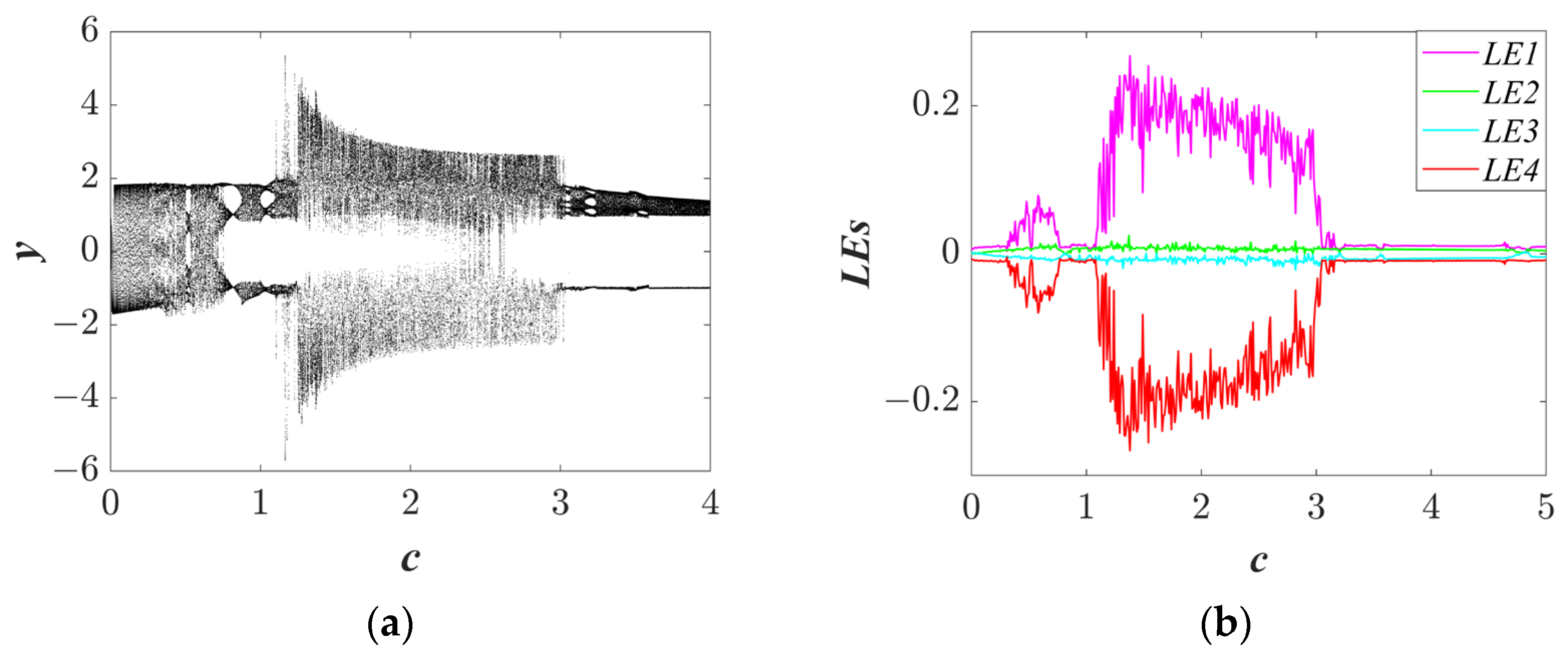
Figure 4.
The bifurcation diagram and Lyapunov exponent spectra of system (3): (a) the bifurcation diagram of c ϵ (0, 4); and (b) the Lyapunov exponent spectra of c ϵ (0, 4).
Figure 4.
The bifurcation diagram and Lyapunov exponent spectra of system (3): (a) the bifurcation diagram of c ϵ (0, 4); and (b) the Lyapunov exponent spectra of c ϵ (0, 4).
Figure 5.
With the parameters a = 1, b = 1, and IC = (1, 0.1, 1, 0.5), the phase portraits vary with the parameter c. (a) c = 0.31; (b) c = 0.38; (c) c = 0.81; and (d) c = 3.7.
Figure 5.
With the parameters a = 1, b = 1, and IC = (1, 0.1, 1, 0.5), the phase portraits vary with the parameter c. (a) c = 0.31; (b) c = 0.38; (c) c = 0.81; and (d) c = 3.7.
Figure 6.
The parameters a = 1.25, b = 1, c = 1, and IC = (0, 0, u, 0) results in the following: (a) the bifurcation diagrams with initial value z(0) = u; and (b) the trajectories at different u values.
Figure 6.
The parameters a = 1.25, b = 1, c = 1, and IC = (0, 0, u, 0) results in the following: (a) the bifurcation diagrams with initial value z(0) = u; and (b) the trajectories at different u values.
Figure 7.
With a = 1, b = 1, and c = 0.81, the basin of attraction at x0 = 1.
Figure 7.
With a = 1, b = 1, and c = 0.81, the basin of attraction at x0 = 1.
Figure 8.
With a = 1, b = 1, and c = 0.81. The phase diagrams at different ICs: (a) IC = (1,0.1,0.1,0.2) and (1,0.1,0.5,0.5); (b) IC = (1,0.1,0.87,0.94) and (1,0.1,1,0.5); (c) IC = (1,0.1,0.6,0.95) and (1,0.1,0.934,1); (d) IC = (1,0.1,0.2,0.8); and (e) IC = (1,0.1,1,0.67).
Figure 8.
With a = 1, b = 1, and c = 0.81. The phase diagrams at different ICs: (a) IC = (1,0.1,0.1,0.2) and (1,0.1,0.5,0.5); (b) IC = (1,0.1,0.87,0.94) and (1,0.1,1,0.5); (c) IC = (1,0.1,0.6,0.95) and (1,0.1,0.934,1); (d) IC = (1,0.1,0.2,0.8); and (e) IC = (1,0.1,1,0.67).
Figure 9.
A schematic diagram of a microcontroller-based digital circuit.
Figure 9.
A schematic diagram of a microcontroller-based digital circuit.
Figure 10.
The experimental result diagrams with a = 1, b = 1, c = 0.81, and IC = (1, 0.1, z0, w0). (a) z0 = 0.2 and w0 = 0.2; (b) z0 = 1 and w0 = 0.5; and (c) z0 = 0.934 and w0 = 1.
Figure 10.
The experimental result diagrams with a = 1, b = 1, c = 0.81, and IC = (1, 0.1, z0, w0). (a) z0 = 0.2 and w0 = 0.2; (b) z0 = 1 and w0 = 0.5; and (c) z0 = 0.934 and w0 = 1.
Figure 11.
Encryption results of images Goldhill, Lena, and Pepper and their histograms. Plain images of (a) Goldhill, (b) Lena, and (c) Pepper; histograms of plain images of (d) Goldhill, (e) Lena, and (f) Pepper; ciphered images of (g) Goldhill, (h) Lena, and (i) Pepper; histograms of ciphered images of (j) Goldhill, (k) Lena; and (l) Pepper.
Table 1.
Results of the NIST test.
Table 1.
Results of the NIST test.
| Statistical Test | p-Value | Result |
|---|
| Monobit | 0.5485 | pass |
| Block Frequency | 0.8862 | pass |
| Runs | 0.6310 | pass |
| Longest Runs | 0.6912 | pass |
| Rank | 0.0352 | pass |
| DFT | 0.7941 | pass |
| Nonoverlapping Template | 0.9754 | pass |
| Overlapping Template | 0.0623 | pass |
| Universal | 0.9118 | pass |
| Linear Complexity | 0.7493 | pass |
| Serial | 0.711 | pass |
| Approximate Entropy | 0.0345 | pass |
| Cumulative Sums | 0.945 | pass |
| Random Excursions | 0.454 | pass |
| Random Excursions Variant | 0.697 | pass |
Table 2.
test.
| Images | Goldhill | Lena | Pepper |
|---|
| plain | 1.6162 × 10⁵ | 1.5835 × 10⁵ | 1.2016 × 10⁵ |
| ciphered | 256.7324 | 186.0684 | 243.4199 |
Table 3.
Correlation coefficients of each image in each direction.
Table 3.
Correlation coefficients of each image in each direction.
| Test Image | Plain Image | Ciphered Image |
|---|
| | Horizontal | Vertical | Diagonal | Horizontal | Vertical | Diagonal |
|---|
| Lena (proposed) | 0.9845 | 0.97 | 0.9632 | −0.0049 | 0.0095 | −0.0106 |
| Lena (ref. [21]) | 0.9850 | 0.9719 | 0.9576 | 0.0231 | 0.0138 | −0.0002 |
| Lena (ref. [22]) | 0.9854 | 0.9736 | 0.9552 | −0.0084 | 0.0065 | 0.0036 |
| Lena (ref. [23]) | 0.9673 | 0.9412 | 0.9132 | 0.0171 | −0.0013 | −0.0005 |
| Lena (ref. [24]) | 0.97688 | 0.9835 | 0.9534 | −0.0088 | 0.0048 | 0.0053 |
| Lena (ref. [25]) | 0.9024 | 0.9287 | 0.8856 | −0.0082 | 0.0094 | 0.0102 |
| Goldhill | 0.974 | 0.9739 | 0.9445 | 0.0049 | −0.0069 | −0.0158 |
| Pepper | 0.9813 | 0.9804 | 0.9676 | −0.0143 | −0.06 | 0.00249 |
Table 4.
Information entropy of test images.
Table 4.
Information entropy of test images.
| Test Image | Plain Image | Ciphered Image |
|---|
| Goldhill | 7.4451 | 7.99936 |
| Pepper | 7.5937 | 7.99928 |
| Pepper (ref. [20]) | 7.6698 | 7.9998 |
| Lena (proposed) | 7.4778 | 7.99933 |
| Lena (ref. [27]) | 7.3982 | 7.9692 |
| Lena (ref. [28]) | 7.5683 | 7.9978 |
| Lena (ref. [29]) | 7.4451 | 7.9993 |
Table 5.
Average local information entropy of test images.
Table 5.
Average local information entropy of test images.
| Test Image | Plain Image | Ciphered Image |
|---|
| Goldhill | 4.7113 | 0.0293 |
| Lena | 4.347 | 0.0282 |
| Pepper | 4.4384 | 0.0308 |
Table 6.
Key sensitivity analysis results.
Table 6.
Key sensitivity analysis results.
| Indicator | Goldhill | Lena | Pepper | Theoretical Value |
|---|
| X0 | NPCR (%) | 99.6096 | 99.6098 | 99.6089 | 99.6094 |
| UACI (%) | 33.4653 | 33.4649 | 33.4653 | 33.4635 |
| BACI (%) | 26.7730 | 26.7714 | 26.7730 | 26.7712 |
| Y0 | NPCR (%) | 99.6097 | 99.6099 | 99.6094 | 99.6094 |
| UACI (%) | 33.4625 | 33.4654 | 33.4605 | 33.4635 |
| BACI (%) | 26.7709 | 26.7709 | 26.7705 | 26.7712 |
| Z0 | NPCR (%) | 99.6089 | 99.6095 | 99.6083 | 99.6094 |
| UACI (%) | 33.4625 | 33.4652 | 33.4633 | 33.4635 |
| BACI (%) | 26.7702 | 26.7709 | 26.7709 | 26.7712 |
| W0 | NPCR (%) | 99.6099 | 99.6089 | 99.6099 | 99.6094 |
| UACI (%) | 33.4640 | 33.4625 | 33.4640 | 33.4635 |
| BACI (%) | 26.7698 | 26.7699 | 26.7798 | 26.7712 |


