Article

On the Possibility of Reproducing Utsu’s Law for Earthquakes with a Spring-Block SOC Model

by
Alfredo Salinas-Martínez
1,*,
Jennifer Perez-Oregon
2,
Ana María Aguilar-Molina
3,
Alejandro Muñoz-Diosdado
3 and
Fernando Angulo-Brown
1,*
1
Departamento de Física, ESFM, Instituto Politécnico Nacional, Mexico City 07738, Mexico
2
Departamento de Ciencias e Ingeniería, Instituto Tecnológico y de Estudios Superiores de Monterrey, Ciudad López Mateos 52926, Edo. de México, Mexico
3
Departamento de Ciencias Básicas, UPIBI, Instituto Politécnico Nacional, Mexico City 07340, Mexico
*
Authors to whom correspondence should be addressed.
Entropy 2023, 25(5), 816; https://doi.org/10.3390/e25050816
Submission received: 4 April 2023 / Revised: 5 May 2023 / Accepted: 6 May 2023 / Published: 18 May 2023

Abstract

:
The Olami, Feder and Christensen (OFC) spring-block model has proven to be a powerful tool for analyzing and comparing synthetic and real earthquakes. This work proposes the possible reproduction of Utsu’s law for earthquakes in the OFC model. Based on our previous works, several simulations characterizing real seismic regions were performed. We located the maximum earthquake in these regions and applied Utsu’s formulae to identify a possible aftershock area and made comparisons between synthetic and real earthquakes. The research compares several equations to calculate the aftershock area and proposes a new one with the available data. Subsequently, the team performed new simulations and chose a mainshock to analyze the behavior of the surrounding events, so as to identify whether they could be catalogued as aftershocks and relate them to the aftershock area previously determined using the formula proposed. Additionally, the spatial location of those events was considered in order to classify them as aftershocks. Finally, we plot the epicenters of the mainshock, and the possible aftershocks comprised in the calculated area resembling the original work of Utsu. Having analyzed the results, it is likely to say that Utsu’s law is reproducible using a spring-block model with a self-organized criticality (SOC) model.

1. Introduction

In the present article we propose a method to estimate the aftershock area given by the Utsu law [1,2] by using the spring-block model suggested by Olami, Feder and Christensen (OFC) [3] based on a bidimensional spring-block array capable of reaching a self-organized criticality (SOC) state. As is well known, the SOC concept was developed by Bak et al. in 1987 [4,5,6,7] and since then this idea has been useful for many applications in several disciplines [8]. The OFC model works as a cellular automaton with a few rules for its evolution (see Section 2.1). The first property known to be reproduced by this model was the Gutenberg—Richter law [9] l o g N ˙ M M 0 = a b M , which relates the magnitude of an earthquake to the number of earthquakes of a given magnitude M , where a is a constant and b is the scaling parameter between large and small events and varies depending on the subduction zone. For several years it was believed that this model did not reproduce aftershocks. However, in 2002 Hergarten and Neugebauer (HN) [10] proposed a manner to obtain aftershocks with the original OFC model.
Aftershocks and their decay have been studied for a long time. Omori proposed in 1894 that they follow a hyperbolic decay with time, following n = k ( c + t ) , which is known as the Omori law [11], where n is the number of aftershocks; k and c are constants that vary between earthquake sequences; and t is the time elapsed since the mainshock. Later, this equation was modified by Utsu in 1961 and took the general form of n = k ( c + t ) p which is known as the Omori-Utsu law [1], where p is a constant that determines the decay rate and can take values between 0.6   a n d   1.1 [12] if the aftershock sequence is modeled by means of a multifractal scaling theory. However, Davidsen et al. [13], by using a generalized Omori-Utsu law, found that the exponent p is a constant > 1 providing convincing evidence that the characteristic time c is not constant but a genuine function of m c , with m c being at a lower magnitude cut off for the aftershocks considered. Some authors have tried to give a generalized form of this law in the form of a differential equation and introduced the idea of a “cool down” process after the mainshock [14,15]. In the end, the goal has been to characterize the behavior of aftershocks so the general activity can be predicted after a big event and therefore, asses the risk in a given zone [16]. In addition, there seems to be a relationship between the parameter b of Gutenberg—Richter and the parameter p of Omori which governs the speed of the aftershock’s decay [17,18,19,20]. So far, we know that the Gutenberg—Richter law is reproducible in the OFC model, so we aimed to see if some sort of Omori-like behavior could be also obtained.
Our group of researchers has studied for a long time the OFC model, trying to reproduce real-seismicity properties reported by seismologists. For our part, we have published several articles in which we found some similarities between the OFC model and real seismicity [3,21,22,23,24,25,26,27,28]. We can outline the ability to emulate real-life seismic subduction zones by including the age of the lithospheric plate and the rate of convergence, both transformed into their synthetic counterparts in the spring-block model [21]; we were also able to reproduce the so-called Ruff—Kanamori diagram [21,23,29] that relates the age of the subduction plate with the convergence rate of the plates and the maximum characteristic earthquake for a given zone. In a different paper, we suggested that the Gutenberg—Richter parameters a and b are positively correlated [24]. We have also published a variation of the OFC model, including non-homogenous cases for different elastic ratios [25,27] and getting the asperity concept into the spring-block model. In the same article, we present an extensive review of our previous results.
In terms of the current study, it aims to replicate Utsu’s law for earthquakes within the OFC model. Additionally, in the spring-block model, there is potential to identify certain events as aftershocks by considering their spatial location.
In the work that our research group has performed, we conducted simulations to study real seismic regions, analyzed the maximum earthquake and identified possible aftershock areas using Utsu’s formulae. We proposed a new equation to calculate the aftershock area and analyzed the behavior of the surrounding events to determine whether they could be classified as aftershocks. By considering the spatial location of these events, we plotted the epicenters of the mainshock and the possible aftershocks within the calculated area, concluding that Utsu’s law is reproducible using a spring-block SOC model.
As for the remaining work, evaluating the suitability of aftershock candidates according to Omori’s law is required. Moreover, exploring the inclusion of the spatial location in identifying potential aftershocks also needs a deeper examination, as we will discuss further.
This article is organized as follows: in Section 2, we present the OFC model and Utsu’s equations. In Section 3, we present the results of the simulations performed to characterize the different seismic regions and the relationship between the different equations to calculate the aftershock area. In Section 4, we discuss the results and analyze them to identify possible aftershocks and the application of the equations for the aftershock area and, finally, in Section 5, we present our conclusions.

2. Methodology

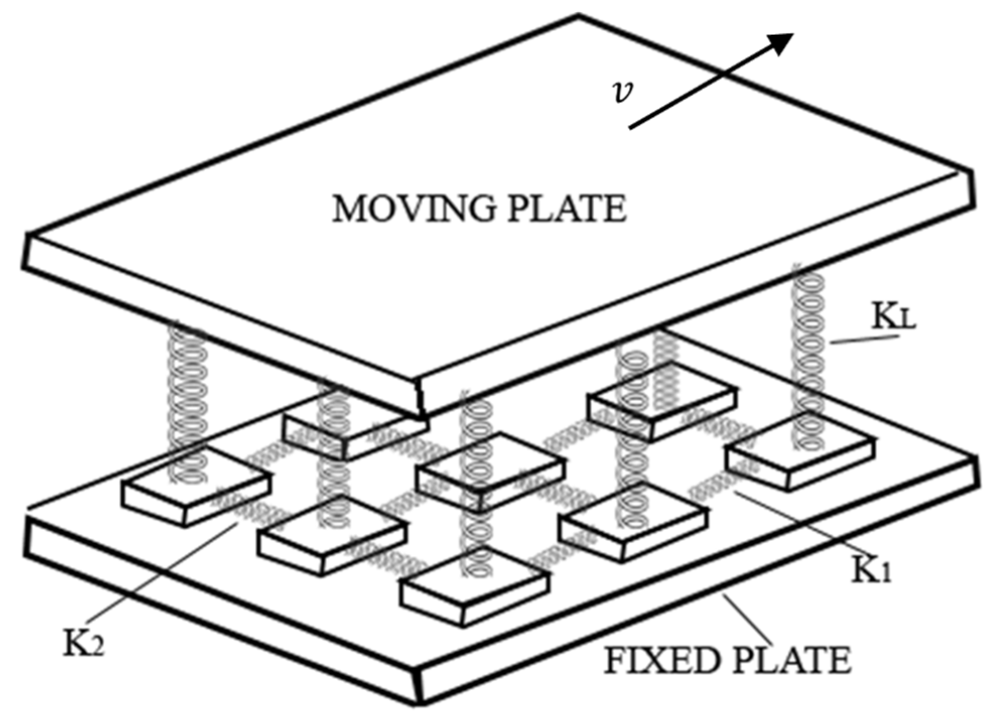
2.1. The Olami-Feder-Christensen Model

The OFC model is characterized as being a non-conservative continuous model that displays self-organized criticality [3]. It is made by a system of blocks interconnected by Hooke springs. Each block is connected to four nearest neighbors. In addition, each of these blocks is connected to a moving plate by another set of Hooke springs and connected to a fixed rigid plate, as shown in Figure 1. The block’s displacement is given by the relative movement between the two plates; when the force in one of the blocks overcomes a certain threshold F t h (the maximum static friction), then the block slips. The moving block then returns to the zero-force position after transferring its energy to the four nearest neighbors which can result in further slips that can provoke a chain reaction.
The spring-block model is a two-dimensional dynamic system composed of interconnected blocks and springs. The blocks are connected to a rigid plate that moves at a constant speed, and the relative motion of the blocks causes them to move as well. Each block has a maximum of four neighbors and will slip if the force acting on it exceeds a certain threshold value. The model can be described using cellular automata, where each block has a force and displacement from its relaxed position on the lattice. The movement of a slipping block can trigger a chain reaction that results in more block movements.
In order to generate the synthetic earthquakes, the spring-block model is mapped to a continuous, non-conservative cellular automaton that follows the next computational evolution rules, as described below.
  • The lattice sites are initialized with random values between zero and a force threshold F t h .
  • The block with the largest force, F m a x , is located, and the difference between F t h and F m a x is added to all sites. This causes a global perturbation.
  • For all sites where F i , j F t h , the force is redistributed among the neighbors of F i , j according to the following rule: F n , n , the forces of the neighboring blocks of the relaxed cell F i , j are increased by γ F i , j , and F i , j is reduced to zero.
  • Step 3 is repeated until the earthquake has fully evolved.
  • Once a state of rest is reached, the process returns to step 2, and synthetic earthquakes are observed until the desired number of events is reached.
The computational rules described before are deduced from the dynamics of the OFC model, which are the following: Consider a network of size L × L , where each block will have a force of F i , j applied to it, with i and j being integers between 1 and L . The displacement of each block from its relaxed position on the lattice will be denoted as x i , j [3].
The total force exerted on a specific block ( i , j ) by the springs can be expressed as:
F i , j = K 1 2 x i , j x i 1 , j x i + 1 , j + K 2 2 x i , j x i , j 1 x i , j + 1 + K L x i , j
where K 1 , K 2 , K L are the elastic constants.
Once a local slip at the position ( i , j ) has happened, the force will redistribute in the following way:
F i ± 1 , j F i ± 1 , j + δ F i ± 1 , j
F i , j ± 1 F i , j ± 1 + δ F i , j ± 1
F i , j 0
where the force increase in the nearest neighbors is given by:
δ F i ± 1 , j = K 1 2 K 1 + 2 K 2 + K L F i , j = γ 1 F i , j
δ F i , j ± 1 = K 2 2 K 1 + 2 K 2 + K L F i , j = γ 2 F i , j
where γ 1 and γ 2 are the elastic ratios.
If K L is greater than 0 , the force redistribution is not conserved, which is expected during actual earthquakes. This results in a redefinition of forces in the nearest-neighbor blocks, which may cause further slipping and trigger a chain reaction or avalanche. For the isotropic case where γ 1 = γ 2 = γ , the OFC model can reproduce the Gutenberg—Richter power law with an exponent similar to the actual one for γ equal to 0.2. Elastic ratios, defined in Equations (5) and (6) can take values between 0 and 0.25. However, the values of the parameter b in the Gutenberg—Richter law that are similar to those observed in real seismicity are only obtained for γ around 0.2.
The magnitude M of a synthetic earthquake will be defined as a function of the number n of relaxed blocks, where M = l o g x ( n ) , and x is the base of the logarithm, in this way the size of the synthetic earthquake is determined by n .
For a more detailed description of the equations and to deepen the choice of elastic parameters, we recommend reading reference [9] where we present an extensive review on this topic.
Based on the work of Perez Oregon et al. [21,22,23], in which they simulated several seismic regions considering the age of the subduction plate and the convergence velocity to reproduce the maximum magnitude earthquake for each region and also using the OFC spring-block model, 29 simulations were performed, same as in [21], using lattices of 100 × 100 blocks and one million iterations. The synthetic age of the subduction zone was obtained considering the interval from 0 to 160 Myr proposed by Ruff and Kanamori [29] and defining e n as the normalized age of the tectonic plates. If we set the value to 1 for the maximum value of the tectonic age (160 Myr) we propose a relation of γ and the tectonic age using [21]:
γ = 0.25 ( 1 e n )
It can be seen that for an old plate γ takes lower values that transform to low-magnitude earthquakes, while for younger ones γ is close to 0.25, which generates high-magnitude earthquakes. For each of the subduction regions considered, the value of γ was calculated. In addition, we included the convergence rate for these plates ranging from 1 to 11.1 cm/year as reported in [23] but converted to the synthetic counterpart ranging from 0 to 3. This synthetic velocity was implemented in the spring-block model by adding it to the difference between F t h F m a x in the first iteration as a global perturbation to obtain the maximum event per simulation.
The magnitude of the synthetic earthquake was determined using the l o g 3 of the size of the earthquake; this size is referred to as the number of relaxed blocks during the simulation. The value of l o g 3 was chosen arbitrarily, and it gives the closest value to real magnitudes [23,25]. We want to emphasize that this l o g value may change if the size of the lattice changes or the number of iterations. Therefore, a new value must be chosen to match the values of real earthquakes. For example, in a 100 × 100 lattice in the case that for a single event all the blocks were relaxed, we would have M = log 3 ( 10000 ) = 8.3 ; while for a 500 × 500 lattice, the same scenario would be M = log 3 ( 250000 ) = 11.3 , which is by far greater than any earthquake reported. In this case, there is a great level of correspondence between the synthetic and the real values of the earthquakes’ magnitudes for each region, as reported in [23,25].

2.2. Utsu’s Law

In its original publication [2], Utsu proposes that every earthquake taking place in a one-month period after the main event and where the magnitude is less than the main event’s magnitude should be considered as an aftershock and not as an isolated event. He also proposes a region in which the epicenters of these aftershocks should be located. This region is called the aftershock area. Utsu [2] defines the aftershock area as the physical area in which the aftershocks are embedded.
The first relationship between the earthquake’s magnitude and the aftershock area was proposed in 1955 by Utsu and Seki [30] as shown in Equation (8):
l o g A = 1.02 M 4.01
where A is the aftershock area in km2, and M is the earthquake magnitude and l o g is a base 10 logarithm.
However, this relation is not unique; for different magnitudes there are different equations which provide a better adjustment. In general, the equations take the general form of l o g A = M β , varying the constants and β according to the case.
For magnitudes M < 7 , he proposes:
l o g A = M 3.7 .
This equation was originally used as a correction of Equation (8) in a zone where the aftershocks exhibit a large scatter [2].
For inland earthquakes, he found that the aftershock area is smaller to offshore earthquakes, and that they fit closer to the following equation:
l o g A = M 4.1 .
This is valid for earthquakes with magnitudes 5.5 M 7.5 .
Goto [31] proposes an equation for the minimum aftershock area for M > 6.5 :
l o g A = 1.74 M 9.92 ,
valid for regions where the seismic activity is low. However, Utsu mentions that the aftershock area given by the latter equation is too small, therefore, he proposes a better adjustment using:
l o g A = M 4.4 ,
which is valid for 5.5 M 8 .
On the other hand, Bath and Buda [32] propose the following relation after analyzing six earthquakes:
l o g A = 1.21 M 5.05
In addition, Purcaru [33] proposes a relation for 5 M 8.5 using the data of fifteen earthquakes:
log A = 1.08 M 4.17

2.3. Aftershocks in the OFC Model

Some researchers [10,34] have pointed out that one of the biggest limitations of the OFC model is the lack of foreshocks or aftershocks, which, in this case, may be difficult to prove that Utsu’s law is present in the OFC model. Some authors have tried to solve this problem. Before, we can mention the work of Hainzl et al. [35] who introduced an additional set of blocks representing the viscous asthenosphere; Pelletier [34], based on Hainzl’s work [35], included heterogeneities into his model. In both cases, they modified the original OFC model and made it more complicated by introducing these new variables. Hergarten and Neugebauer [10] did a statistical analysis of the time series in the OFC model and proposed a method to classify events after the mainshock as aftershocks. They proposed to use the time (number of events) between what they consider successive mainshocks of the same or larger magnitude as the recurrence time. Then, they set a window to limit where to look for aftershocks. After this, as long as the following events are not bigger than the mainshock and are located within this window, they are considered aftershocks.

3. Results

3.1. Utsu’s Law Simulations

In Figure 2, we show one of the cases in the original work of Utsu where the main shock is illustrated as a double circle while the aftershock area is the dashed line ellipse, all the events that fulfill the requirements of time and magnitude are considered aftershocks [2]. The relative position of the main shock with respect to the aftershocks in the twenty-five cases reported by Utsu in [1] are located in some cases at the edges of the respective area, but in many of them they are located practically in the middle of the area. For the spring-block simulation, we take into consideration that the relaxed elements in our simulations can be identified graphically, and these elements generate a “relaxed area” equivalent to the size of the synthetic earthquake (Figure 3); we propose the equivalence between the synthetic earthquake’s size and Utsu’s aftershock area. When a synthetic earthquake occurs, the relaxed area has many blocks that are near the threshold, therefore, the probability that the following earthquakes occur in that area is high, which is in consonance with real seismicity. Based on this, we take the relaxed area as equivalent to the aftershock area in the Utsu construction.
In order to compare the real magnitude (the maximum magnitude reported in a given seismic region) and the real aftershock area versus the synthetic magnitude and the synthetic aftershock area, we treated real earthquakes’ magnitudes as synthetic ones in a spring-block simulation so we can expect a certain size (synthetic) for those events (where this size is the number of relaxed elements in a simulation). Since we already have emulated 29 subduction seismic zones [21,25], it was easy to apply the following transformation for going from real seismicity to synthetic seismicity:
Expected   Size S ^ = 3 M
Afterwards, we calculated the aftershock area using Equations (8)–(14) and (16) (see below) as shown in Table 1. Table 1 lists the maximum real earthquake’s magnitude reported for each one of the twenty-nine subduction seismic regions that were used in [21]. We highlighted the equation that gives the closest value to the expected size calculated with Equation (16) so the reader can identify the best fit for each case. This comparison was made only with Equations (8)–(14). In addition, we obtained a new equation using linear regression for this data set. The resultant equation was:
log A = 0.477 M
It is worth mentioning that our proposed Equation (16) is the one closest to the expected size in comparison to the rest of Equations (8)–(14) and it is the reason the comparison mentioned earlier did not include Equation (16). As the magnitude increases, the difference between the expected size and the fit given by Equations (8)–(14) also increases dramatically. On the other hand, that difference remains minimal with Equation (16).
In Table 1, we present the results for the maximum earthquake’s magnitude reported (real seismicity), while in Table 2 are the results for the spring-block simulations of each seismic region (synthetic seismicity). For Table 2, we present the maximum synthetic size which was obtained with the spring-block simulation and then the equivalent magnitude was computed with Equation (15) and solved for M . The reader might notice that the same magnitude has associated different values of the synthetic size; this is the result of rounding Equation (15) to one decimal position. In both cases, as previously stated, the earthquake’s size is equivalent to the aftershock area, so this value should be approximated by any of the Equations (8)–(14). We highlighted the computed aftershock area that is the closest to the earthquake’s size by comparing Equations (8)–(14) so the reader can identify the best fit for each magnitude.
In Table 1, according to our data model, a particular equation fits more accurately to a certain magnitude range. For magnitudes M < 7.6 , the closest result is given by Equation (8); while in the range of 7.6 M 8 , the best adjustment is given by Equation (10) and for magnitudes over 8, the best adjustment is given by Equation (12). However, it is important to mention that, in all ranges in our proposal, Equation (16) is almost equal to the expected size.
In Table 2, since there are slight variations in the synthetic earthquakes (for example, we have the lowest magnitude value of 6.8 in comparison with 7.5 in Table 1) the equations also have variations over the range they fit the best. We can see that for M = 6.8 , Equation (13) gives the best adjustment; on the other hand, for M = 7.2 we have two adjustments (again, given by the rounding of Equation (15)), the first is given by Equation (9), and the second one by Equation (8). The behavior for M 7.6 is identical to the one in Table 1. For the synthetic catalog, we found that in our proposal, Equation (16) gives the most accurate value for the synthetic size.
In Figure 4, we show a projection of Equations (8)–(14) and (16) for magnitudes 5 M 9.5 vs. the l o g 3 of the synthetic size in the spring-block model. On the one hand, it can be noticed that in the range of 6.7 M 8.1 several equations are very close to the expected size (the × symbol in Figure 4), however, Equations (8)–(14) overestimate the aftershock area for magnitudes M > 8.1 while underestimating it for magnitudes below 6. On the other hand, Equation (16) (the □ symbol in Figure 4) follows with a 1% difference in the values of the expected size. We want to emphasize that this equation was derived using the data obtained from the spring-block model, which can be said is the equation governing the synthetic size, and that is why it follows almost perfectly the tendency of the expected size.
In Table 1 and Table 2, we notice that as the magnitude increases, the difference between the computed and the expected value of the aftershock area also increases. In Table 1, the difference in percentage ranges from 15.48% (for M = 7.5 ) to 270.25% (for M = 9.5 ). Therefore, a better adjustment is needed. For Equation (16), this error ranges from 0.21% (for M = 7.5 ) to 0.26% (for M = 9.5 ). On the other hand, in Table 2, the error for the best fit ranges from 8.4% (for M = 6.8 ) to 297% (for M = 9.6 ), while for Equation (16) the error ranges from 0.16% (for M = 6.8 ) to 0.26% (for M = 9.6 ).

3.2. Aftershocks and Utsu’s Law in a Spring-Block Model

In Section 2.3, we mentioned the difficulties in accurately reproducing aftershocks in the OFC model and some attempts to statistically identify events as aftershocks. We used a methodology similar to the one used by HN [10] to determine if an event is an aftershock or if it is an isolated event. They used a lattice of 512 × 512 and 10 9 events. Then, they defined the minimum value for an event to be considered as a mainshock in the time of the mainshock t M , which was 1000 blocks, and it had to be the greatest event in an interval of [ t M 10 4 , t M + 10 4 ]. The next step was to monitor the number of events in a fixed window and subtract the background seismic activity. We used a 100 × 100 model with one million iterations. In Figure 5, we show the time series for the model, the x axis represents the consecutive event number, and since the time between events is always the same (one iteration), the number of events can be considered also as the timestamp. The y axis represents the synthetic size of that earthquake and expresses the total number of relaxed blocks for that iteration. It is worth mentioning that for the first 400 thousand events, they seem to follow an exponential growth before reaching the SOC state. To make the analysis, we had to determine how big an event must be to be classified as a mainshock, we decided to choose only the events whose sizes were 3000 and above that represent a magnitude of 7.2 which is just below the lowest value of the maximum earthquake reported for the subduction regions. Then we chose one of those events and tried to use a window of 104 elements. However, this window was proven to be inefficient since in many cases we found another mainshock inside those 104 elements. So, we decided to use instead of a fixed window just the space between consecutive mainshocks (events with at least 3000 blocks) and tried to elucidate how many of those events could be catalogued as aftershocks.
One crucial difference between our method and the HN one [10] is that they count all the events inside the window without taking into consideration how far they are from the mainshock’s epicenter, while we wanted to relate the event number and its spatial position. For this purpose, we set an arbitrary radius of 40 blocks to delimit the area where to find aftershocks. In Figure 6, we show the time series of the aftershocks’ candidates inside this ring. Then we plot all of these events in an x , y plane as shown in Figure 7. Notice that the events are spread throughout the entire lattice, so it is obvious that not all of them can be considered aftershocks. As mentioned before, we decided to set a radius of 40 (dashed line in Figure 7) choosing the mainshock’s epicenter as the circle’s center, as in many cases presented by Utsu [2]. Once we had this delimitation, we had to eliminate all the events that can be considered as background noise. We set this limit to 27, which is equivalent to events of magnitude M = 3 .
Then we decided to apply Equation (16) to refine the aftershock area. This new area is shown in Figure 7 as a solid line circle. The mainshock is marked with a small red circle. Events in black hexagons are discarded as aftershocks since they are too far away from the mainshock’s epicenter. The dashed line represents the original area arbitrarily chosen, while the solid line represents Utsu’s aftershock area obtained using Equation (16). Green diamonds were discarded as they represent background noise. Blue stars are the aftershocks candidates.
It is important to mention that many of the biggest events in the interval analyzed were located far away from the mainshock’s epicenter and therefore were discarded as aftershocks.
In Figure 8, we present an image of the aftershocks candidates after cleaning the background noise and removing the elements outside the rings. It can be seen that even though we removed several events, we still have enough events enclosed within the rings. What is more, the inner ring, which corresponds to the aftershock area computed with Equation (16), has 216 possible aftershocks which seem reasonable for an earthquake of magnitude M ~ 7 . Finally, in Figure 9, we show the time series of those events.

4. Discussion

We generated 29 simulations using the OFC model with a 100 × 100 lattice and one million iterations, as in references [5,9]. We applied Equations (8)–(14) for the aftershock area proposed by Utsu and Seki [30], Utsu [2], Goto [31], Bath and Buda [32], and Purcaru [33] to both catalogs: synthetic and real subduction zones as reported in [21]. Finally, we used the data generated by the spring-block model to derive our own Equation (16).
From Table 1 and Table 2, and Figure 4, we observed that when using Equations (8)–(14) the error increases along with the magnitude in both scenarios: real and synthetic. This situation makes it clear that a new fit is necessary. This led us to the proposal of Equation (16). The errors related to this equation are on the order of 0.2 % . It is clear that for both cases, the best equation to approximate the size of the event is Equation (16). This might stand, therefore, as an indicator that validates this proposal. Although this result was obtained using the spring-block model, its application to real events (complete data sets) is yet to be analyzed.
Regarding the identification of aftershocks candidates in the spring-block model, we believe that it is possible that we can classify some events as aftershocks, especially if we use, as a discriminant analysis, the spatial location and not only the recurrence time. However, we admit that there is a lot of work to do on this matter, especially since we have not proven that these candidates follow Omori’s law for aftershocks [11]. From Figure 9, one might rush and say that they follow a hyperbolic decay. Data from Figure 9 is kind of reminiscent of Omori’s law, where the cumulative size of the aftershocks decays with time following the equation y = 5270.2 t 0.578 as illustrated in Figure 10. The behavior of the aftershocks is remarkably similar to Omori’s law with the difference that we do not show the decay in the number of events but in their cumulative size (this size as mentioned earlier is the number of relaxed blocks per event). Eventually, they become small enough to be considered as part of the background activity, similar to the real-life seismic activity.

5. Conclusions

We conclude that it seems possible to qualitatively reproduce Utsu’s law using the OFC spring-block model due to the similarities between the actual seismic regions compared to the simulations. It is clear that a single equation cannot fit all ranges of magnitudes in real scenarios. For the synthetic case, we propose an Equation (16) that fits the expected values very well. This does not mean that the same behavior can be expected in real seismicity since we used synthetic catalogs to derive that equation, but it does make clear the need for a better spring-block model that qualitatively approaches the real-life seismicity. With this, we are not saying that the current model is not valid. It is important to remember that this is a model that works with quite simple rules and does not include many of the parameters observed in real seismicity. However, it fulfills the function of qualitatively reproducing many of the empirical laws and behaviors found in the real world, and for this study, it provides a good approximation for certain quantities where all other equations seem to work well.
Finally, although our results seem to confirm that Utsu’s law can be reproduced in the spring-block model, a deeper analysis of the possible replications in the OFC model is necessary. In addition, the inclusion of spatial location when identifying possible aftershocks brings us closer to a more complete model of earthquakes. It should be noted that these results are promising regarding the use of the spring-block model and its ability to reproduce complex properties of the seismic phenomenon.

Author Contributions

Conceptualization, F.A.-B. and A.M.-D.; investigation, A.S.-M., A.M.A.-M., J.P.-O., F.A.-B. and A.M.-D.; methodology, A.S.-M., A.M.A.-M., J.P.-O., F.A.-B. and A.M.-D.; software, A.S.-M., A.M.A.-M. and J.P.-O.; supervision, A.M.-D.; writing—original draft, A.S.-M., A.M.A.-M., J.P.-O., F.A.-B. and A.M.-D.; writing—review and editing, A.S.-M., A.M.A.-M., J.P.-O., F.A.-B. and A.M.-D. All authors have read and agreed to the published version of the manuscript.

Funding

This research was funded by SIP-IPN-20231637.

Institutional Review Board Statement

Not applicable.

Data Availability Statement

Synthetic data can be provided by writing to the corresponding author.

Acknowledgments

A.M.-D and F.A.-B. acknowledge COFAA-IPN, EDI-IPN, and SNI-CONACyT-MEXICO. A.M.A.-M. and A.S.M. thank CONACyT-MEXICO for partial support.

Conflicts of Interest

The authors declare no conflict of interest.

References

  1. Utsu, T. A statistical study on the occurrence of aftershocks. Geophys. Mag. 1961, 30, 521–605. [Google Scholar]
  2. Utsu, T. Aftershocks and Earthquake Statistics (1): Some Parameters Which Characterize an Aftershock Sequence and Their Interrelations. J. Fac. Sci. Hokkaido Univ. Ser. 7 Geophys. 1970, 3, 129–195. [Google Scholar]
  3. Olami, Z.; Feder, H.; Christensen, K. Self-Organized Criticality in a Continuous, Nonconservative Cellular Automaton Modeling Earthquakes. Phys. Rev. Lett. 1992, 68, 1244–1247. [Google Scholar] [CrossRef] [PubMed]
  4. Bak, P.; Tang, C.; Wiesenfeld, K. Self-organized criticality: An explanation of the 1/f noise. Phys. Rev. Lett. 1987, 59, 381. [Google Scholar] [CrossRef]
  5. Bak, P.; Tang, C.; Wiesenfeld, K. Self-organized criticality. Phys. Rev. A 1988, 38, 364. [Google Scholar] [CrossRef] [PubMed]
  6. Bak, P.; Tang, C. Earthquakes as a Self-Organized Critical Phenomenon. J. Geophys. Res. 1989, B94, 15635. [Google Scholar] [CrossRef]
  7. Bak, P. How Nature Works; Springer Science: New York, NY, USA, 1996. [Google Scholar]
  8. Watkins, N.W.; Pruessner, G.; Chapman, S.C.; Crosby, N.B.; Jensen, H.J. 25 Years of Self-organized Criticality: Concepts and Controversies. Space Sci. Rev. 2016, 198, 3–44. [Google Scholar] [CrossRef]
  9. Gutenberg, B.; Richter, C.F. Frequency of earthquakes in California. Bull. Seismol. Soc. Am. 1944, 34, 185–188. [Google Scholar] [CrossRef]
  10. Hergarten, S.; Neugebauer, H.J. Foreshocks and aftershocks in the Olami-Feder-Christensen Model. Phys. Rev. Lett. 2002, 88, 238501. [Google Scholar] [CrossRef]
  11. Omori, F. On the aftershocks of earthquakes. J. Coll. Sci. Imp. Univ. Tokyo 1894, 7, 111–200. [Google Scholar]
  12. Sornette, D.; Ouillon, G. Multifractal Scaling of Thermally Activated Rupture Processes. Phys. Rev. Lett. 2005, 94, 038501. [Google Scholar] [CrossRef] [PubMed]
  13. Davidsen, J.; Gu, C.; Baiesi, M. Generalized Omori–Utsu law for aftershock sequences in southern California. Geoph. J. Int. 2015, 201, 965–978. [Google Scholar] [CrossRef]
  14. Guglielmi, A.V. Interpretation of the Omori law. Izv. Phys. Solid Earth 2016, 52, 785–786. [Google Scholar] [CrossRef]
  15. Guglielmi, A.V.; Zavyalov, A.D. The Omori Law: The 150-Year Birthday Jubilee of Fusakichi Omori. J. Volcanolog. Seismol. 2018, 12, 353–358. [Google Scholar] [CrossRef]
  16. Baranov, S.; Narteau, C.; Shebalin, P. Modeling and Prediction of Aftershock Activity. Surv. Geophys. 2022, 43, 437–481. [Google Scholar] [CrossRef]
  17. Wang, J.-H. On the correlation of observed Gutenberg-Richter’s b value and Omori’s p value for aftershocks. Bull. Seismol. Soc. Am. 1994, 84, 2008–2011. [Google Scholar] [CrossRef]
  18. Helmstetter, A.; Sornette, D. Subcritical and supercritical regimes in epidemic models of earthquake aftershocks. J. Geophys. Res. Solid Earth 2002, 107, ESE-10. [Google Scholar] [CrossRef]
  19. Guo, Z.; Ogata, Y. Statistical relations between the parameters of aftershocks in time, space, and magnitude. J. Geophys. Res. Solid Earth 1997, 102, 2857–2873. [Google Scholar] [CrossRef]
  20. Zaccagnino, D.; Telesca, L.; Doglioni, C. Scaling properties of seismicity and faulting. Earth Planet. Sci. Lett. 2022, 584, 117511. [Google Scholar] [CrossRef]
  21. Perez Oregon, J.; Muñoz Diosdado, A.; Rudolf-Navarro, A.H.; Angulo-Brown, F. A simple model to relate the elastic ratio gamma of a critically self-organized spring-block model with the age of a lithospheric downgoing plate in a subduction zone. Entropy 2020, 7, 868. [Google Scholar] [CrossRef]
  22. Perez Oregon, J. On some Little-Known Properties of the Gutenberg-Richter Relationship for the Frequency of Earthquakes. Ph.D. Thesis, Instituto Politécnico Nacional, ESFM, Mexico City, Mexico, 2018. [Google Scholar]
  23. Perez-Oregon, J.; Muñoz-Diosdado, A.; Rudolf-Navarro, A.H.; Angulo-Brown, F. Some Common Features Between a Spring-Block Self-Organized Critical Model, Stick–Slip Experiments with Sandpapers and Actual Seismicity. Pure Appl. Geophys. 2020, 177, 889–903. [Google Scholar] [CrossRef]
  24. Perez-Oregon, J.; Muñoz-Diosdado, A.; Rudolf-Navarro, A.H.; Guzman-Saenz, A.; Angulo-Brown, F. On the possible correlation between the Gutenberg-Richter parameters of the frequency-magnitude relationship. J. Seism. 2018, 22, 1025–1035. [Google Scholar] [CrossRef]
  25. Salinas-Martínez, A.; Aguilar-Molina, A.M.; Pérez-Oregon, J.; Angulo-Brown, F.; Muñoz-Diosdado, A. Review and Update on Some Connections between a Spring-Block SOC Model and Actual Seismicity in the Case of Subduction Zones. Entropy 2022, 24, 435. [Google Scholar] [CrossRef] [PubMed]
  26. Muñoz-Diosdado, A.; Angulo-Brown, F. Patterns of synthetic seismicity and recurrence times in a spring-block earthquake model. Rev. Mex. Fís. 1999, 45, 393–400. [Google Scholar]
  27. Muñoz-Diosdado, A.; Rudolf-Navarro, A.H.; Angulo-Brown, F. Simulation and properties of a non-homogeneous spring-block earthquake model with asperities. Acta Geophys. 2012, 60, 740–757. [Google Scholar] [CrossRef]
  28. Muñoz Diosdado, A.; Rudolf-Navarro, A.H.; Angulo Brown, F. A qualitative comparison between some synthetic and empirical scaling properties in seismicity. Rev. Mex. Fís. S 2012, 58, 96–103. [Google Scholar]
  29. Ruff, L.; Kanamori, H. Seismicity and the subduction process. Phys. Earth Planet. Inter. 1980, 23, 240–252. [Google Scholar] [CrossRef]
  30. Utsu, T.; Seki, A. Relation between the area of aftershock region and the energy of the main shock. J. Seism. Soc. Jap. 1955, 7, 233–240. [Google Scholar]
  31. Goto, K. On the relation between the distribution of aftershocks and the magnitude. J. Seism. Soc. Jap. 1962, 15, 116–121. [Google Scholar]
  32. Bath, M.; Buda, S.I. Earthquake volume, fault plane area, seismic energy, strain, deformation, and related quantities. Ann. Geofis. 1964, 17, 363–368. [Google Scholar]
  33. Purcaru, G. Some problems of the Vrancea earthquakes and their aftershocks. St. Cerc. Geol. Geofiz. Geogr. Ser. Geofiz. 1966, 4, 87–99. [Google Scholar]
  34. Pelletier, J.D. GeoComplexity and the Physics of Earthquakes; Rundle, J.B., Turcotte, D.L., Klein, W., Eds.; American Geophysical Union: Washington, DC, USA, 2000; pp. 27–42. [Google Scholar]
  35. Hainzl, S.; Zöller, G.; Kurths, J. Similar power laws for fore- and aftershock sequences in a spring-block model for earthquakes. J. Geophys. Res. 1999, 104, 7243. [Google Scholar] [CrossRef]
Figure 1. Schematics for the spring-block model.
Entropy 25 00816 g001
Figure 2. The ellipse in the dashed line represents the aftershock area proposed by Utsu. All the events with epicenters inside this ellipse are considered aftershocks of the main event that is marked as a double circle. Image taken from [1].
Entropy 25 00816 g002
Figure 3. Relaxed area in a spring-block simulation. The earthquake’s epicenter is shown as a black dot in the black circle. L is the size of the lattice, γ is the elastic parameter or conservation level [24].
Entropy 25 00816 g003
Figure 4. Magnitude vs. l o g 3 (expected size) given by Equations (8)–(14).
Entropy 25 00816 g004
Figure 5. Time series of synthetic earthquakes in the OFC spring-block model.
Entropy 25 00816 g005
Figure 6. Time series of aftershocks candidates.
Entropy 25 00816 g006
Figure 7. X Y plot of all the events between two mainshocks. The dash line represents the initial chosen area while solid line is the aftershock area calculated with Equation (16). Grey hexagons represent all the events that lie outside the rings; green diamonds represent the background noise; blue stars represent the aftershocks candidates.
Entropy 25 00816 g007
Figure 8. Aftershocks candidates after removing background noise and far away events.
Entropy 25 00816 g008
Figure 9. Aftershocks candidates’ series after removing far away events and background noise.
Entropy 25 00816 g009
Figure 10. Aftershocks decay with time. The dotted red line represents the adjusted decay over time that follows y = 5270.2 t 0.578 .
Entropy 25 00816 g010
Table 1. Comparison of the aftershock area given by Equations (8)–(14) using the maximum real earthquake’s magnitudes reported in each seismic region. The expected size was computed by using Equation (15). The closest value to the expected size is highlighted in green. The last column is the result of our proposed Equation (16), which gives the best approximation to the expected size.
Subduction
Seismic Region
MExpected SizeEquation (8)Equation (9)Equation (10)Equation (11)Equation (12)Equation (13)Equation (14)Equation (16)
Caribbean7.537884365631025121349125910,59385113780
Marianas7.537884365631025121349125910,59385113780
Scotia arc7.642285521794331622014158513,99610,9144219
S. Java7.74719698210,00039813006199518,49313,9964709
New Zealand7.85267883112,58950124487251224,43417,9475255
Patagonia7.85267883112,58950124487251224,43417,9475255
Vanatu (New Hebrides)7.9587811,16915,84963106699316232,28523,0145865
Izu Bonin7.9587811,1691584963106699316232,28523,0145865
Kermadec7.9587811,16915,84963106699316232,28523,0145865
México-Oaxaca7.9587811,16915,84963106699316232,28523,0145865
México-Guerrero7.9587811,16915,84963106699316232,28523,0145865
Ryukyus86,56114,12519,953794310,000398142,65829,5126546
Tonga8.1732317,86525,11910,00014,928501256,36437,8447306
Peru8.1732317,86525,11910,00014,928501256,36437,8447306
Central America8.1732317,86525,11910,00014,928501256,36437,8447306
Mexico-Michoacán8.1732317,86525,11910,00014,928501256,36437,8447306
W. Alaska8.2817322,59431,62312,58922,284631074,47348,5298155
México- Jalisco8.2817322,59431,62312,58922,284631074,47348,5298155
Sumba Island8.3912228,57639,81115,84933,266794398,40162,2309101
Kuriles8.511,36445,70963,09625,11974,13112,589171,791102,32911,337
West Aleutians8.612,68457,81079,43331,623110,66215,849226,986131,22012,653
Komandorski8.714,15673,114100,00039,811165,19619,953299,916168,26714,122
Central Chile8.815,80092,470125,89350,119246,60425,119396,278215,77415,762
Colombia-Ecuador8.815,80092,470125,89350,119246,60425,119396,278215,77415,762
Kamchatka919,683147,911199,52679,433549,54139,811691,831354,81319,634
NE Japan9.121,969187,068251,189100,000820,35250,119914,113454,98821,913
Sumatra-Andaman9.224,520236,592316,228125,8931,224,61663,0961,207,814583,44524,457
East Alaska9.224,520236,592316,228125,8931,224,61663,0961,207,814583,44524,457
South Chile9.534,092478,630630,957251,1894,073,803125,8932,786,1211,230,26934,002
Table 2. Comparison of the aftershock area given by Equations (8)–(14) using the spring-block model. For each simulation, we obtained the maximum synthetic size of a given region, then the magnitude M was computed applying Equation (15) and solving for M = log 3 S ^ . The closest value to the expected size is highlighted in green. The last column is the result of our proposed Equation (16), which gives the best approximation to the synthetic size.
Subduction Seismic RegionMSynthetic SizeEquation (8)Equation (9)Equation (10)Equation (11)Equation (12)Equation (13)Equation (14)Equation (16)
Caribbean6.81832924137654895275167816441829
Marianas7.22738218131951272413638465040822732
Scotia arc7.22786226333141319440661486042462780
Vanatu (New Hebrides)7.641875407778330991944155313,65510,6774178
Izu Bonin7.642165488789731441993157613,89610,8454207
S. Java7.745616493931237072655185816,96412,9594551
Kermadec7.745986606947137702735189017,31513,1984588
New Zealand7.746106643952337912761190017,43013,2764600
Sumba Island7.85175850512,13448314209242123,36917,2475164
Patagonia8.0629812,94218,31372918614365438,45426,9026284
Tonga8.1709916,71823,536937013,330469652,09635,2767083
NE Japan8.2795921,34729,91011,90820,227596869,62245,6977941
Kuriles8.2840523,98633,53113,34924,677669079,94651,7008386
Ryukyus8.3904328,04739,08815,56132,223779996,24561,0129022
Kamchatka8999434,73248,20219,19046,4029618124,02576,5099971
W. Alaska8.410,05435,17948,81119,43247,4269739125,92377,55310,030
Komandorski8.410,12435,70549,52619,71748,6419882128,15878,78010,100
Sumatra-Andaman8.410,28336,91451,17020,37151,48610,210133,32481,60910,259
West Aleutians8.410,35237,44651,89220,65952,75710,354135,60482,85310,328
Peru8.410,57239,16854,23121,59056,96210,820143,03386,89310,547
East Alaska8.613,08461,78184,77933,751123,94416,916245,601140,78413,053
Central America8.714,30174,719102,15240,667171,43120,382307,743172,18114,266
Central Chile8.815,02082,980113,21345,071205,01222,589348,509192,40114,983
México-Oaxaca8.918,605131,131177,30970,588447,49935,378599,742312,34118,559
México-Guerrero9.121,842184,770248,16398,795803,23549,515900,807449,07221,787
Mexico-Michoacán9.326,583281,198374,578149,1221,644,23274,7381,482,470700,52826,514
Colombia-Ecuador928,450325,111431,843171,9202,106,04086,1641,760,938816,86828,376
México-Jalisco9.429,780358,469475,240189,1972,487,87994,8231,977,267905,87129,702
South Chile9.636,428551,485724,982288,6215,187,635144,6533,296,0661,429,39936,331
Disclaimer/Publisher’s Note: The statements, opinions and data contained in all publications are solely those of the individual author(s) and contributor(s) and not of MDPI and/or the editor(s). MDPI and/or the editor(s) disclaim responsibility for any injury to people or property resulting from any ideas, methods, instructions or products referred to in the content.

