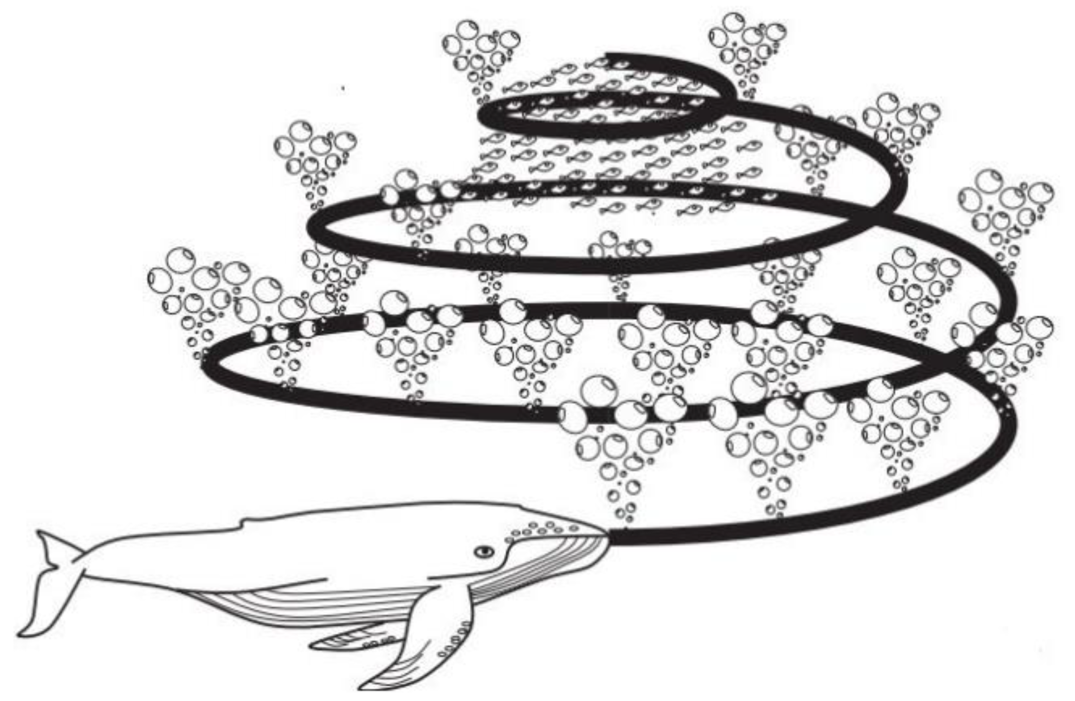
Figure 1.
Humpback whales simulate “bubble net” feeding behavior.
Figure 1.
Humpback whales simulate “bubble net” feeding behavior.
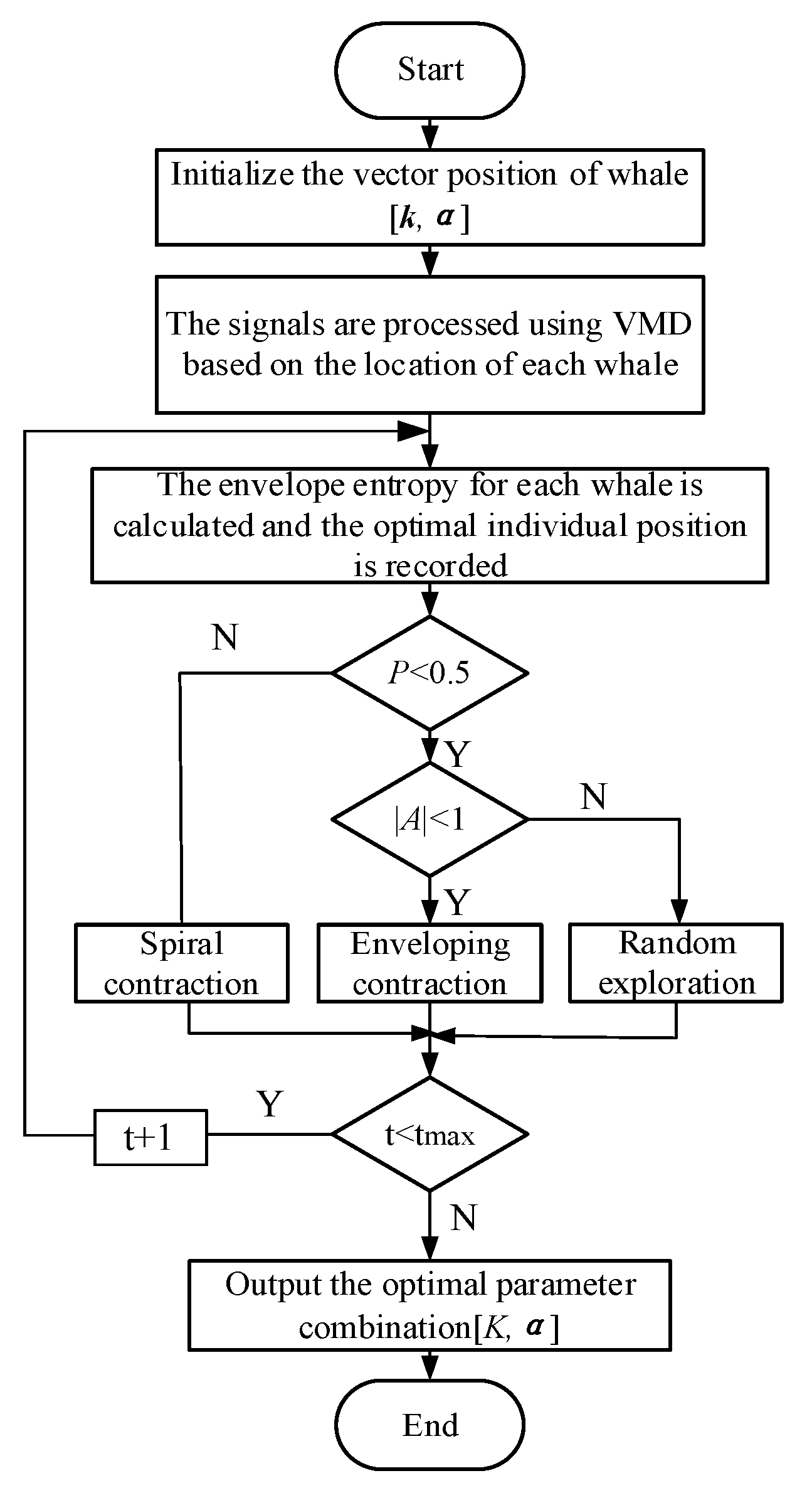
Figure 2.
WOA Optimization Process.
Figure 2.
WOA Optimization Process.
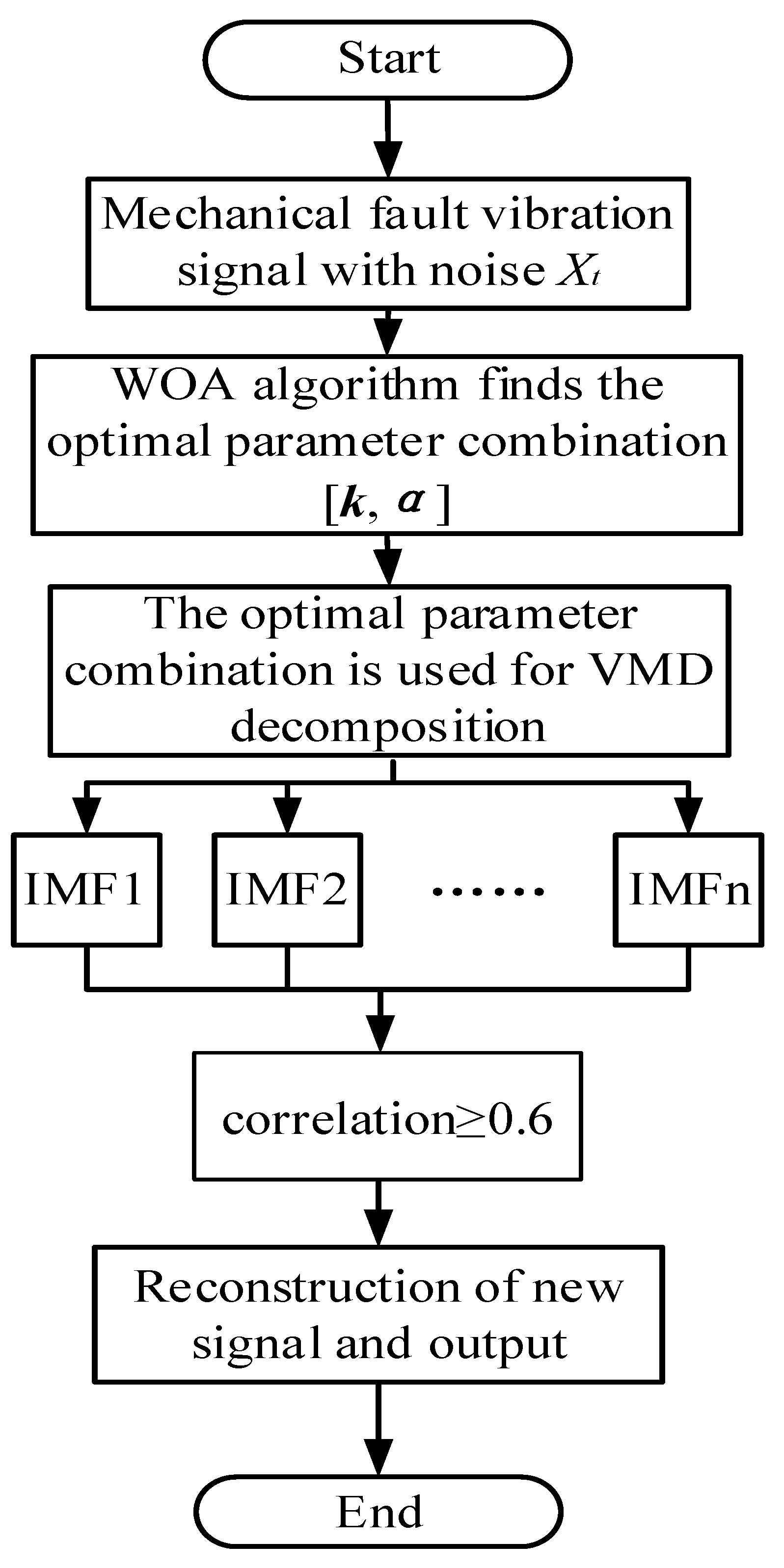
Figure 3.
WOA-VMD-based signal noise reduction process.
Figure 3.
WOA-VMD-based signal noise reduction process.
Figure 4.
Construct an example of adjacency matrix based on KNN.
Figure 4.
Construct an example of adjacency matrix based on KNN.
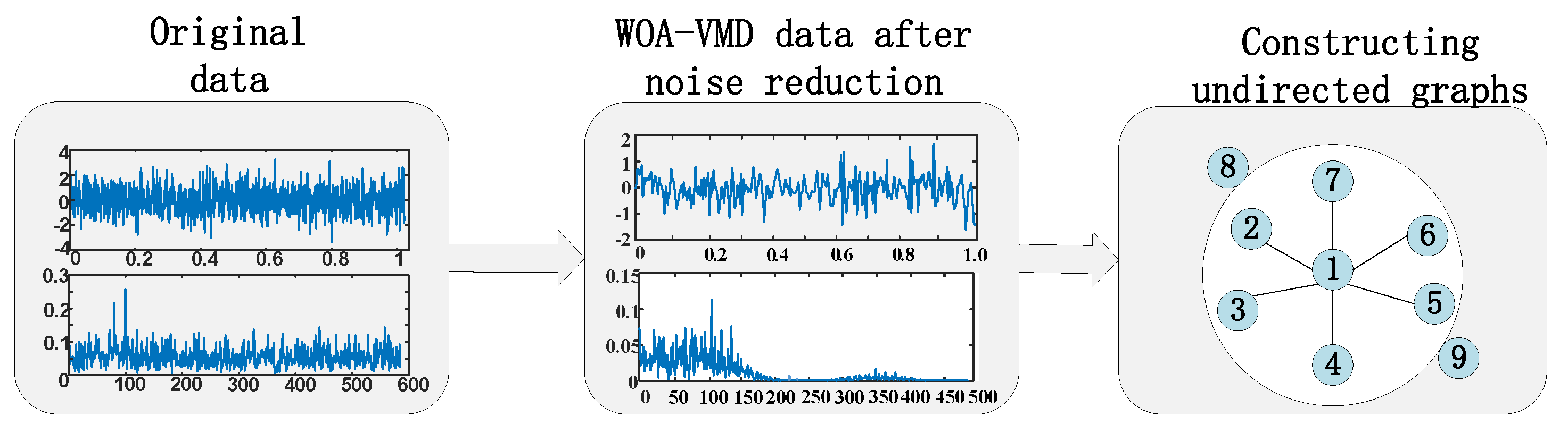
Figure 5.
Composition process of the undirected graph of fault data.
Figure 5.
Composition process of the undirected graph of fault data.
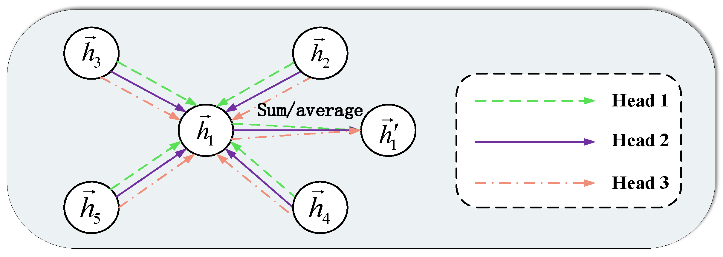
Figure 6.
Multi-head attention mechanism schematic diagram.
Figure 6.
Multi-head attention mechanism schematic diagram.
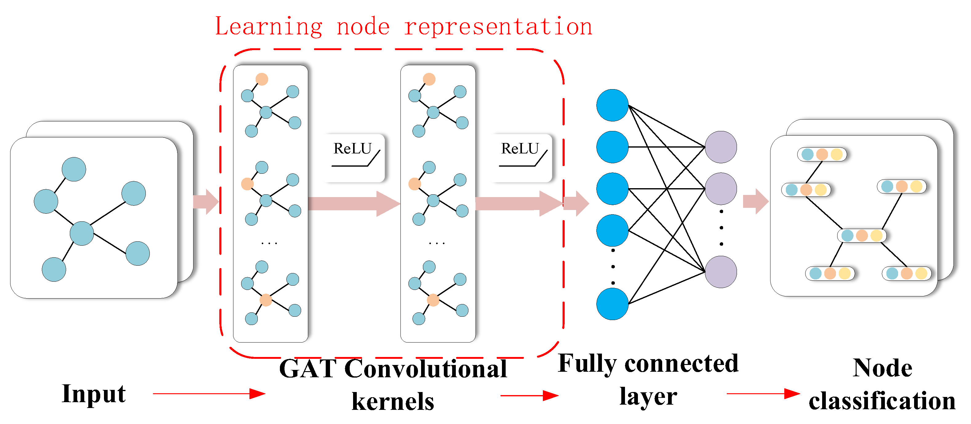
Figure 7.
Diagram of GAT model.
Figure 7.
Diagram of GAT model.
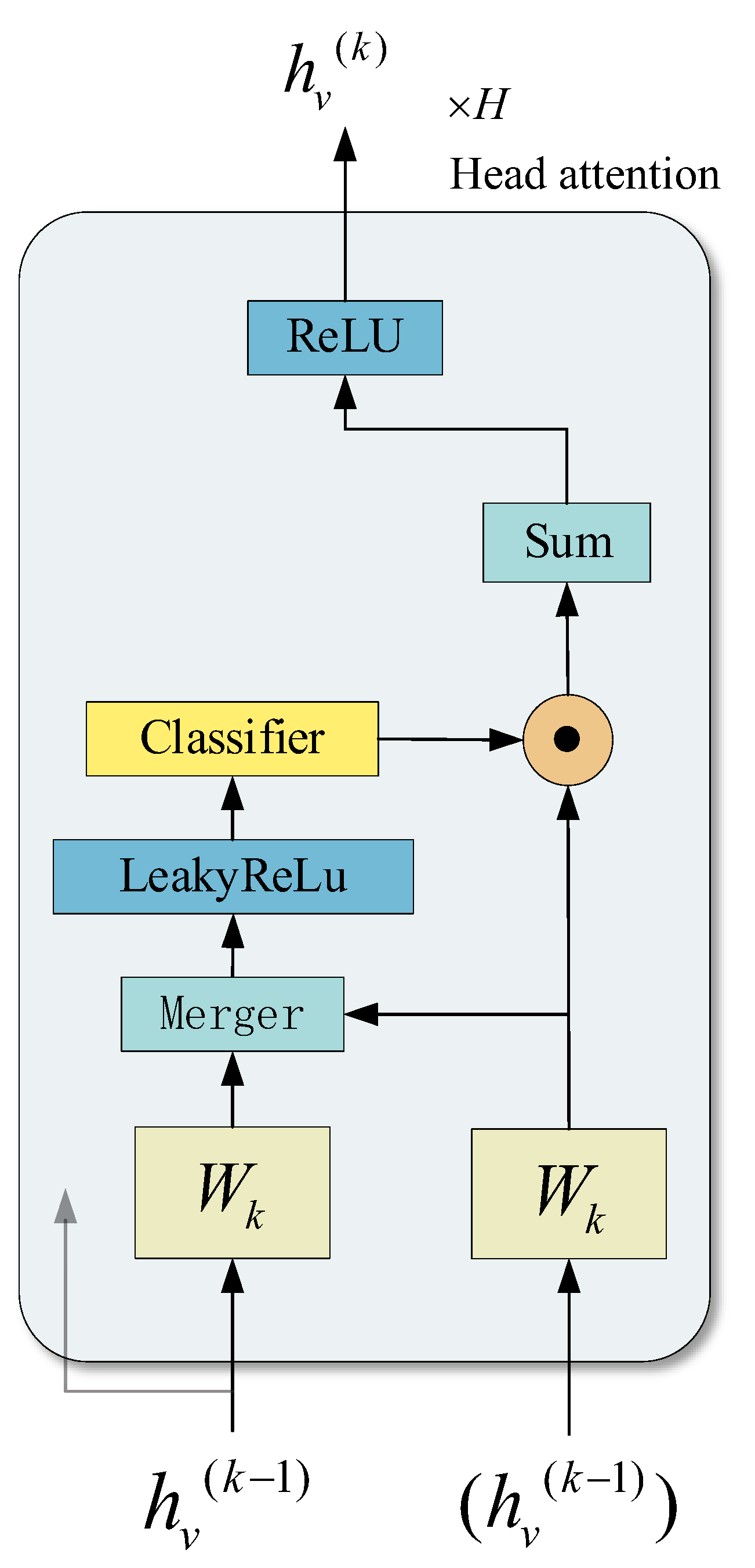
Figure 8.
Schematic diagram of GAT layer structure.
Figure 8.
Schematic diagram of GAT layer structure.
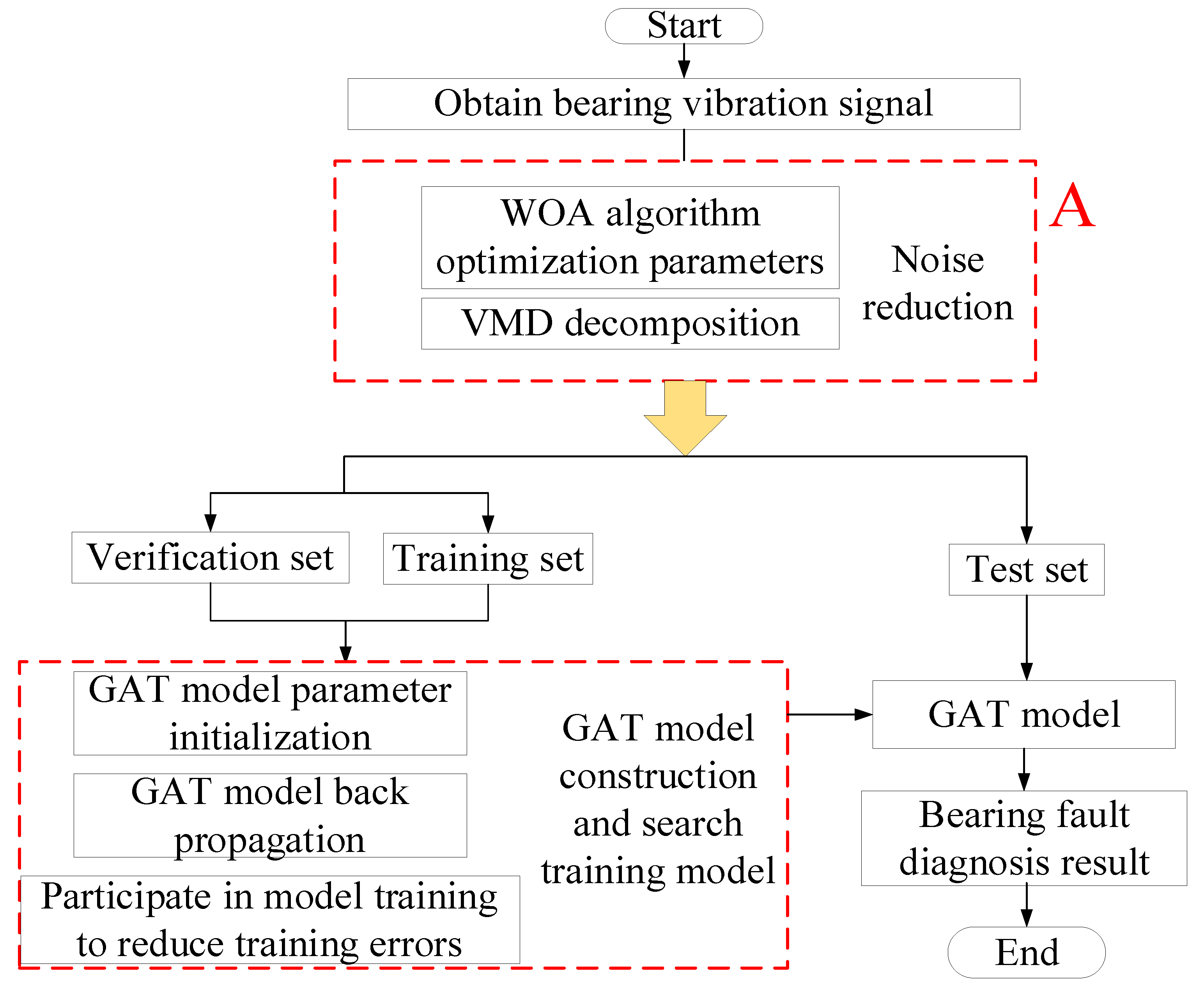
Figure 9.
Fault diagnosis flow chart.
Figure 9.
Fault diagnosis flow chart.
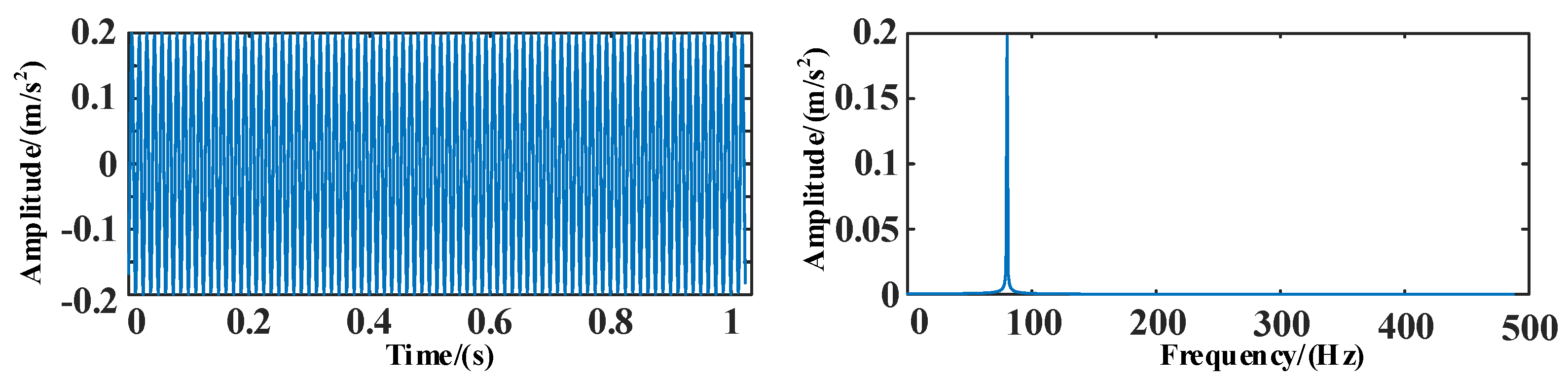
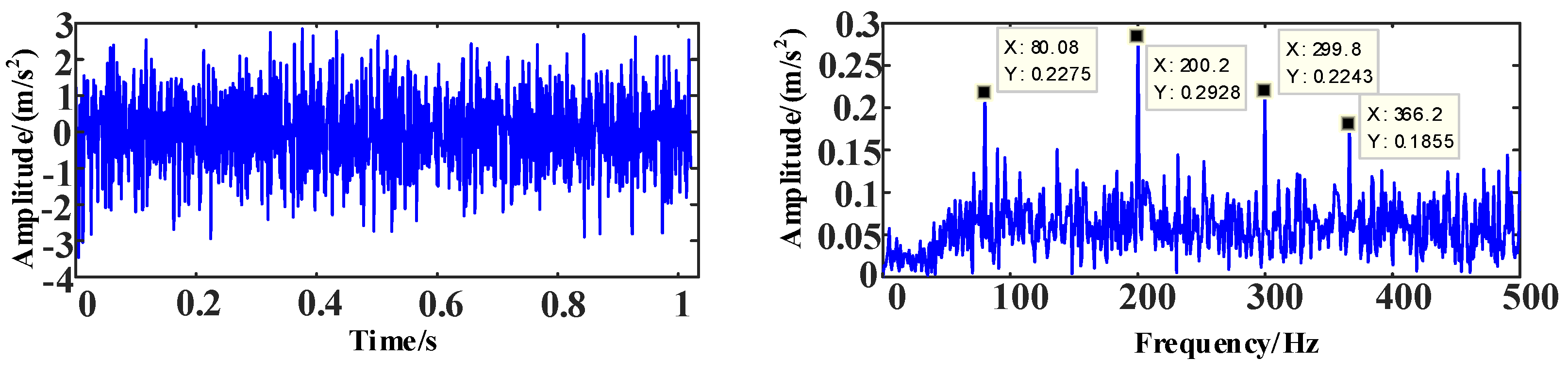
Figure 10.
The time and frequency domain diagrams of signal s1.
Figure 10.
The time and frequency domain diagrams of signal s1.
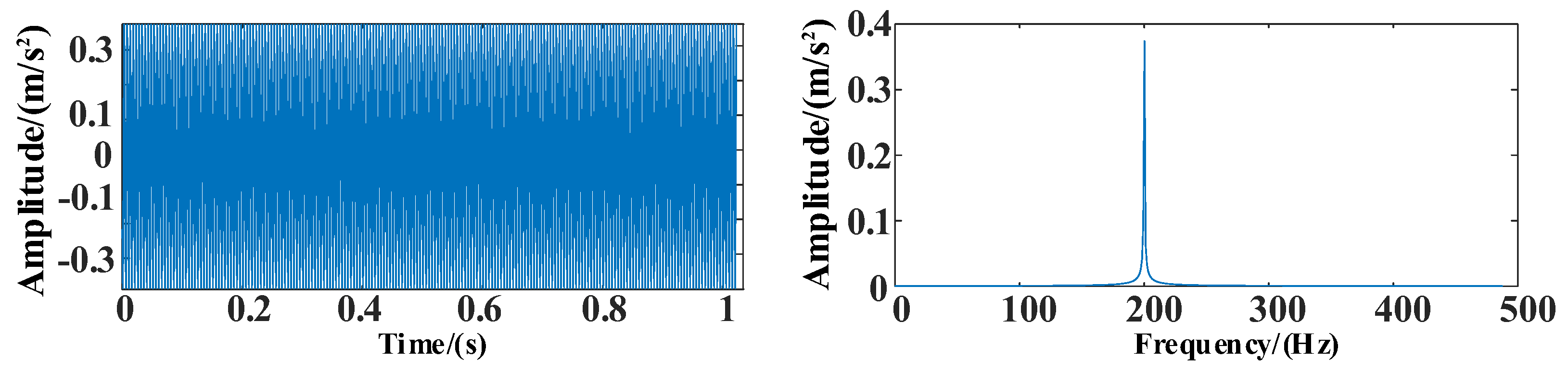
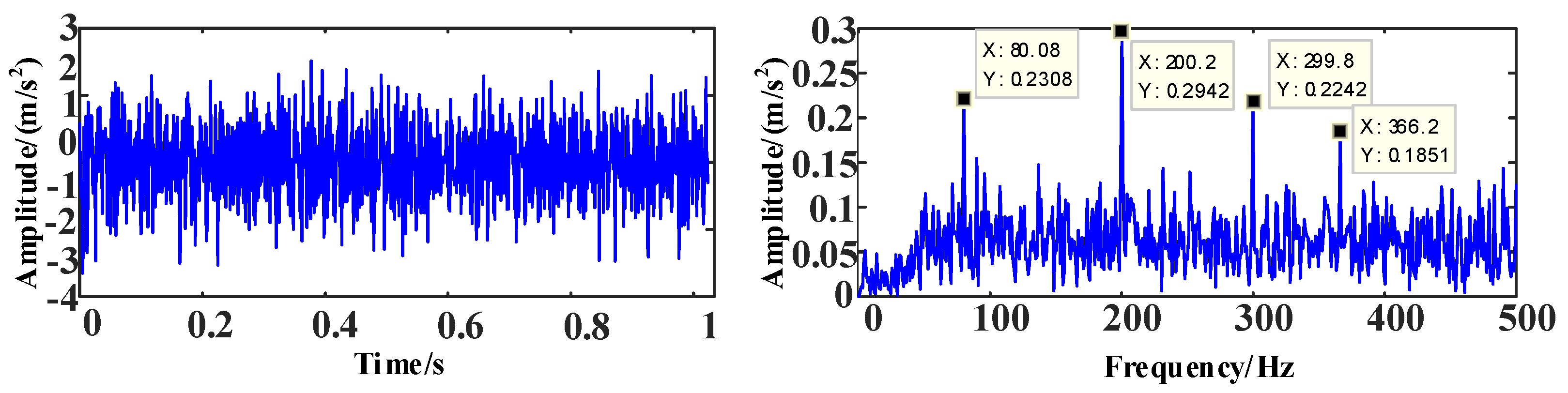
Figure 11.
The time and frequency domain diagrams of signal s2.
Figure 11.
The time and frequency domain diagrams of signal s2.
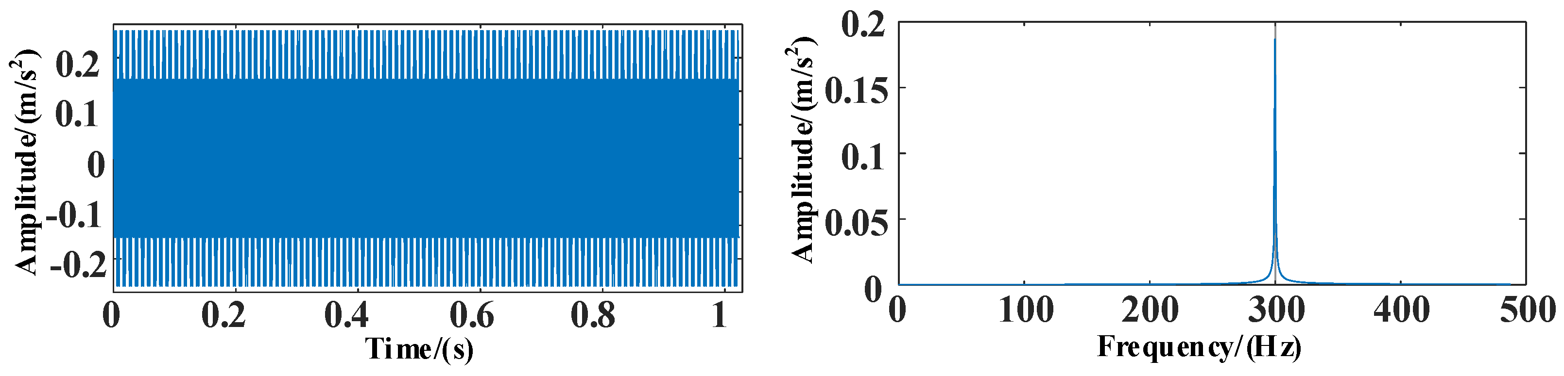
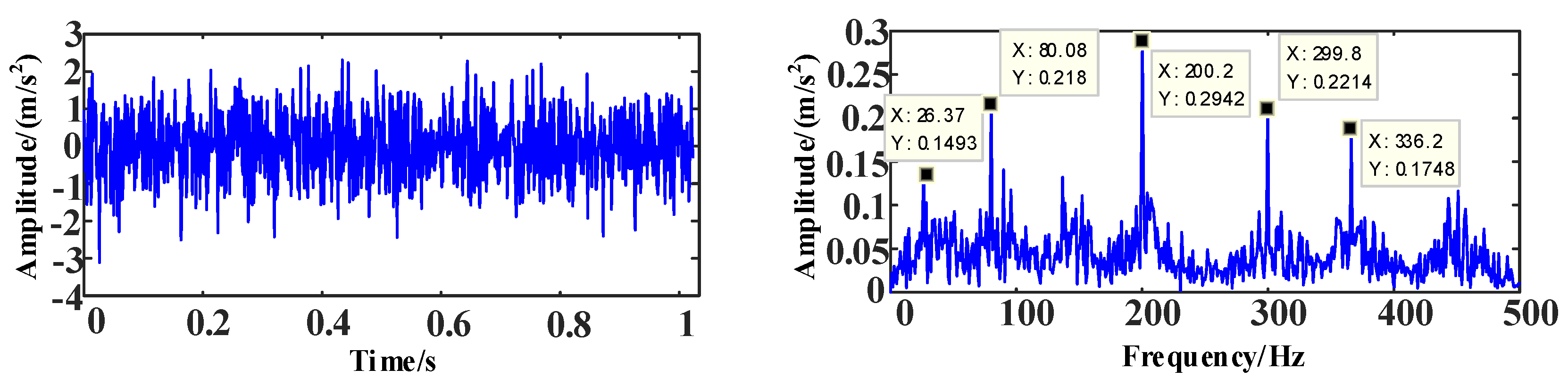
Figure 12.
The time and frequency domain diagrams of signal s3.
Figure 12.
The time and frequency domain diagrams of signal s3.
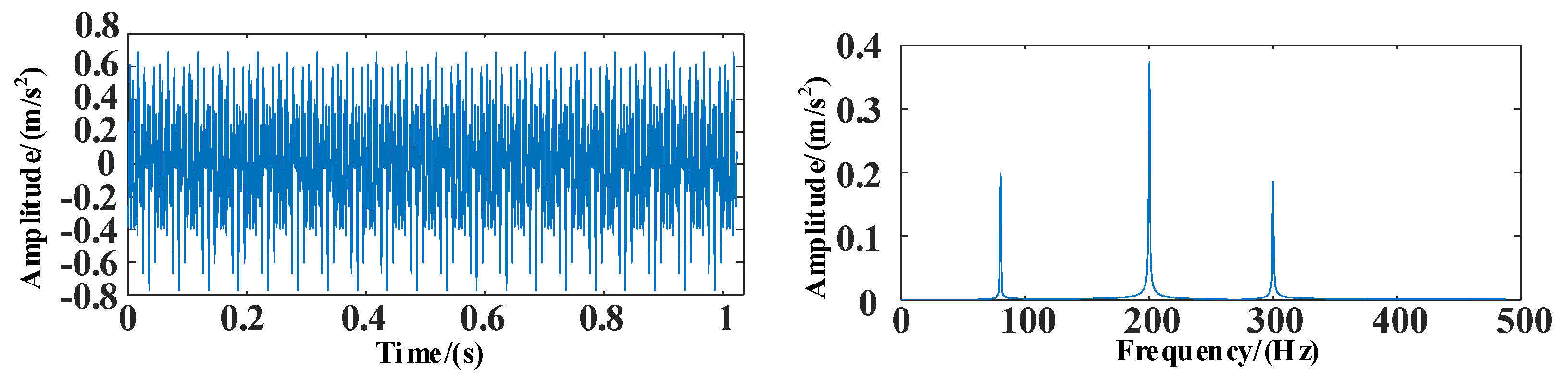
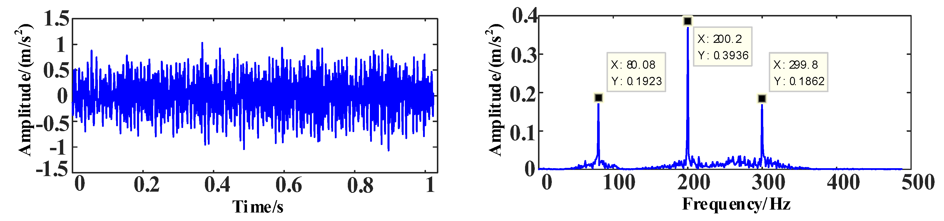
Figure 13.
The time and frequency domain diagrams of signal Z.
Figure 13.
The time and frequency domain diagrams of signal Z.
Figure 14.
The time and frequency domain diagrams of signal after noise addition.
Figure 14.
The time and frequency domain diagrams of signal after noise addition.
Figure 15.
WOA-VMD iteration curve. (a) Optimization process curve of penalty factor; (b) Optimization process curve of decomposition mode number; (c) Envelope entropy iteration curve of WOA.
Figure 15.
WOA-VMD iteration curve. (a) Optimization process curve of penalty factor; (b) Optimization process curve of decomposition mode number; (c) Envelope entropy iteration curve of WOA.
Figure 16.
The time and frequency domain diagram of IMF after WOA-VMD decomposition.
Figure 16.
The time and frequency domain diagram of IMF after WOA-VMD decomposition.
Figure 17.
The time and frequency domain diagrams of EMD noise reduction.
Figure 17.
The time and frequency domain diagrams of EMD noise reduction.
Figure 18.
The time and frequency domain diagrams of EEMD noise reduction.
Figure 18.
The time and frequency domain diagrams of EEMD noise reduction.
Figure 19.
The time and frequency domain diagrams of CEEMD noise reduction.
Figure 19.
The time and frequency domain diagrams of CEEMD noise reduction.
Figure 20.
The time and frequency domain diagrams of GA-VMD noise reduction.
Figure 20.
The time and frequency domain diagrams of GA-VMD noise reduction.
Figure 21.
The time and frequency domain diagrams of WOA-VMD noise reduction.
Figure 21.
The time and frequency domain diagrams of WOA-VMD noise reduction.
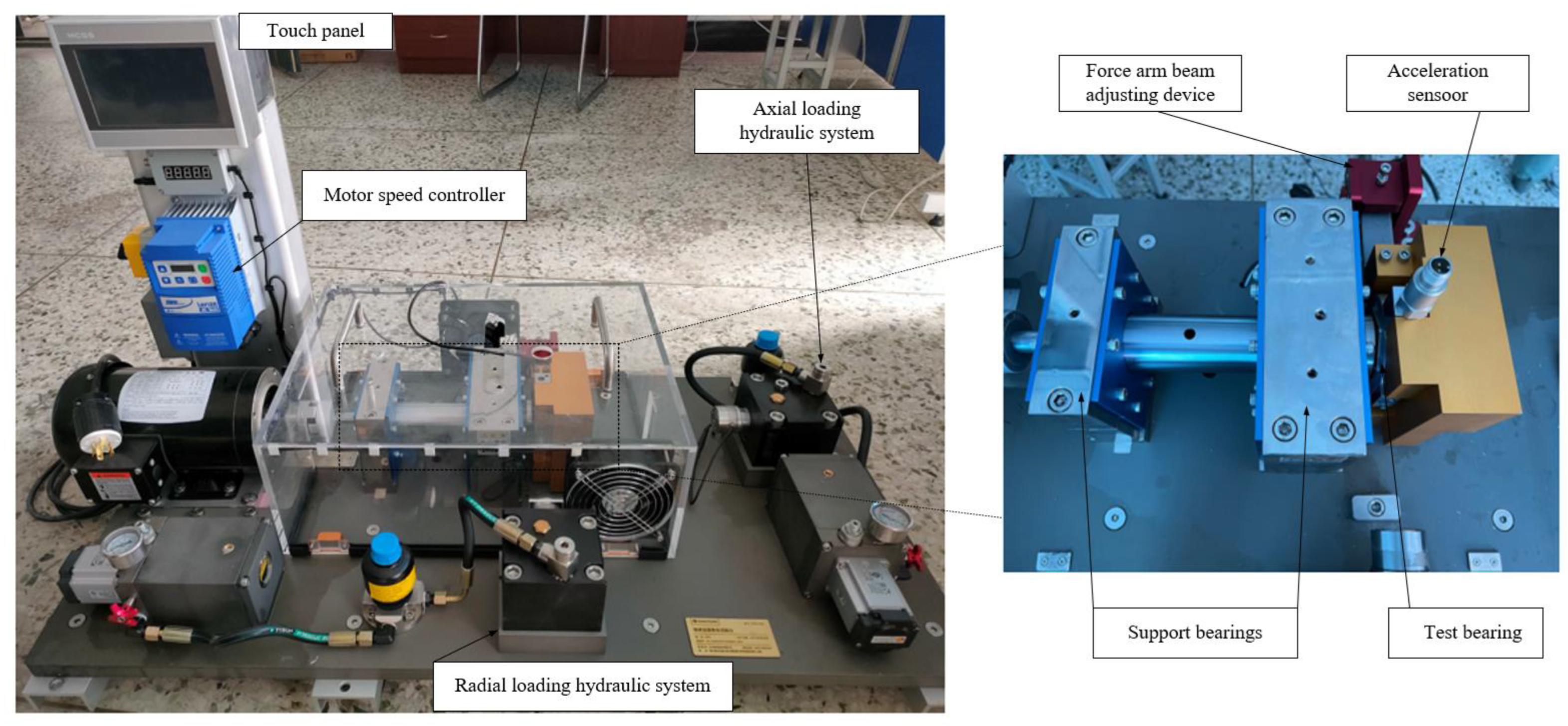
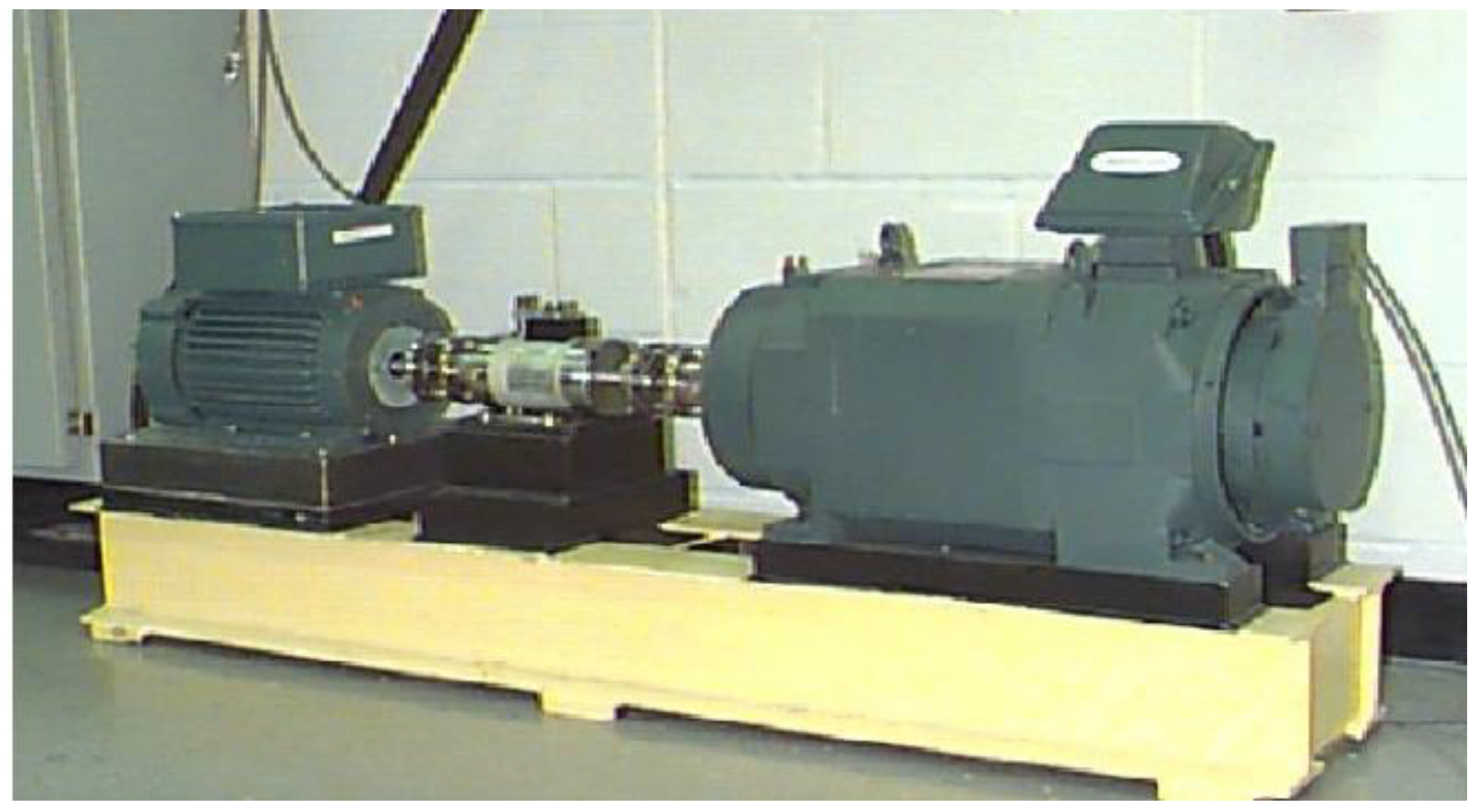
Figure 22.
Test bench for rolling bearings.
Figure 22.
Test bench for rolling bearings.
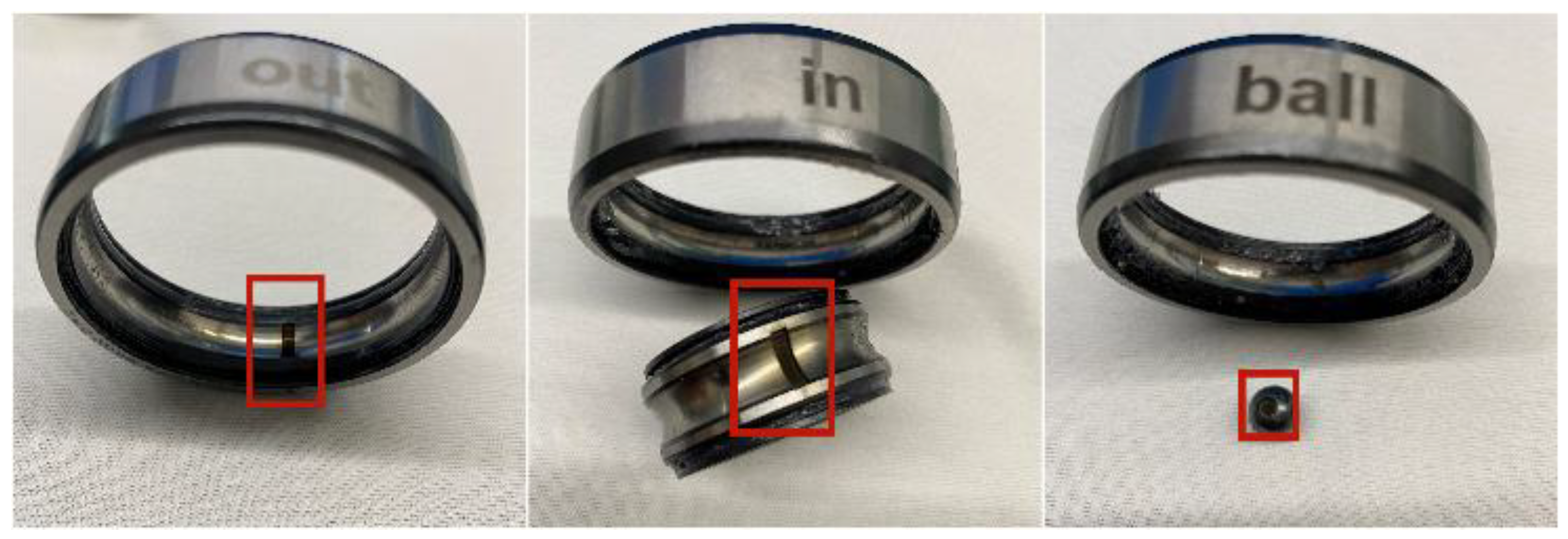
Figure 23.
Damage diagrams of rolling bearings.
Figure 23.
Damage diagrams of rolling bearings.
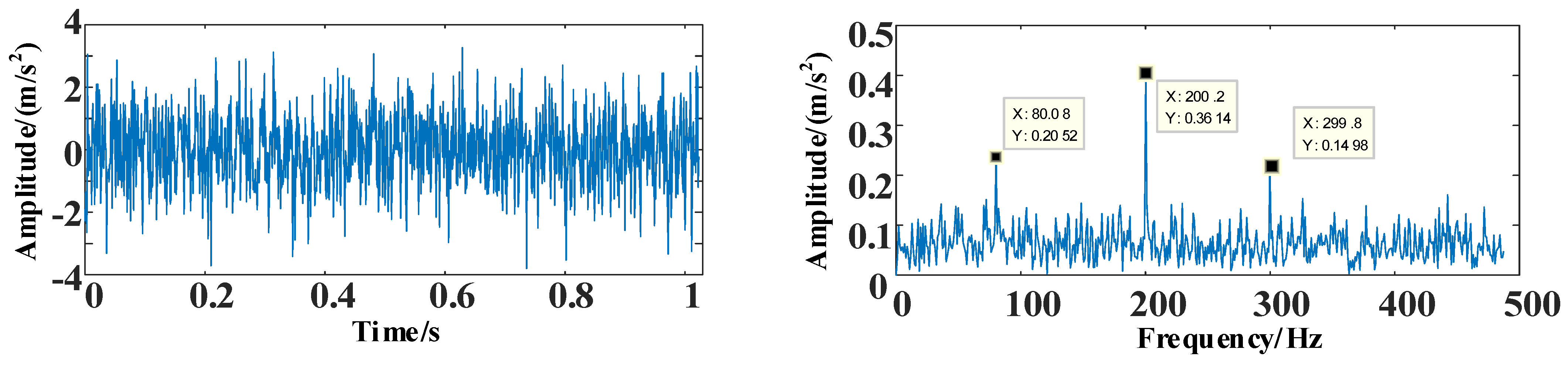
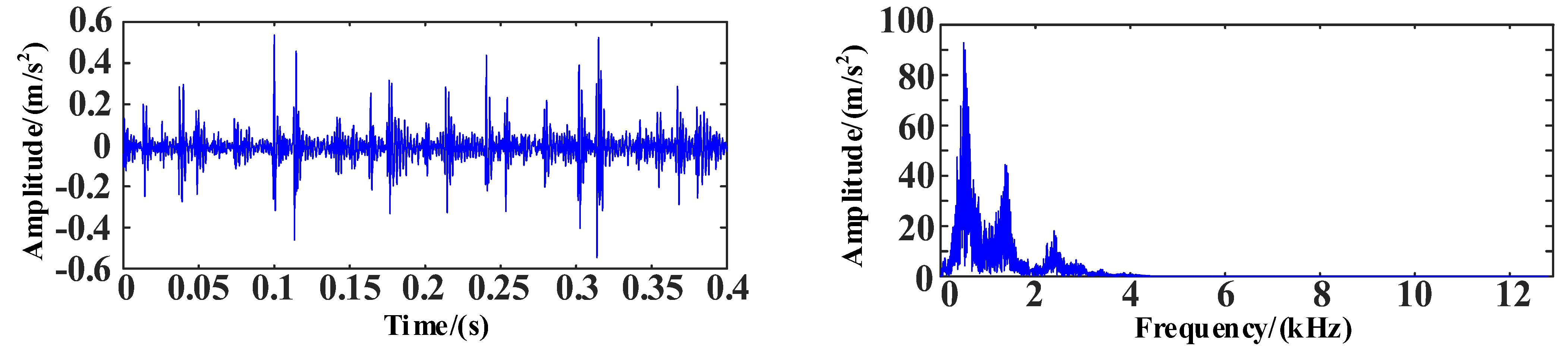
Figure 24.
The time and frequency domain diagrams of vibration signals.
Figure 24.
The time and frequency domain diagrams of vibration signals.
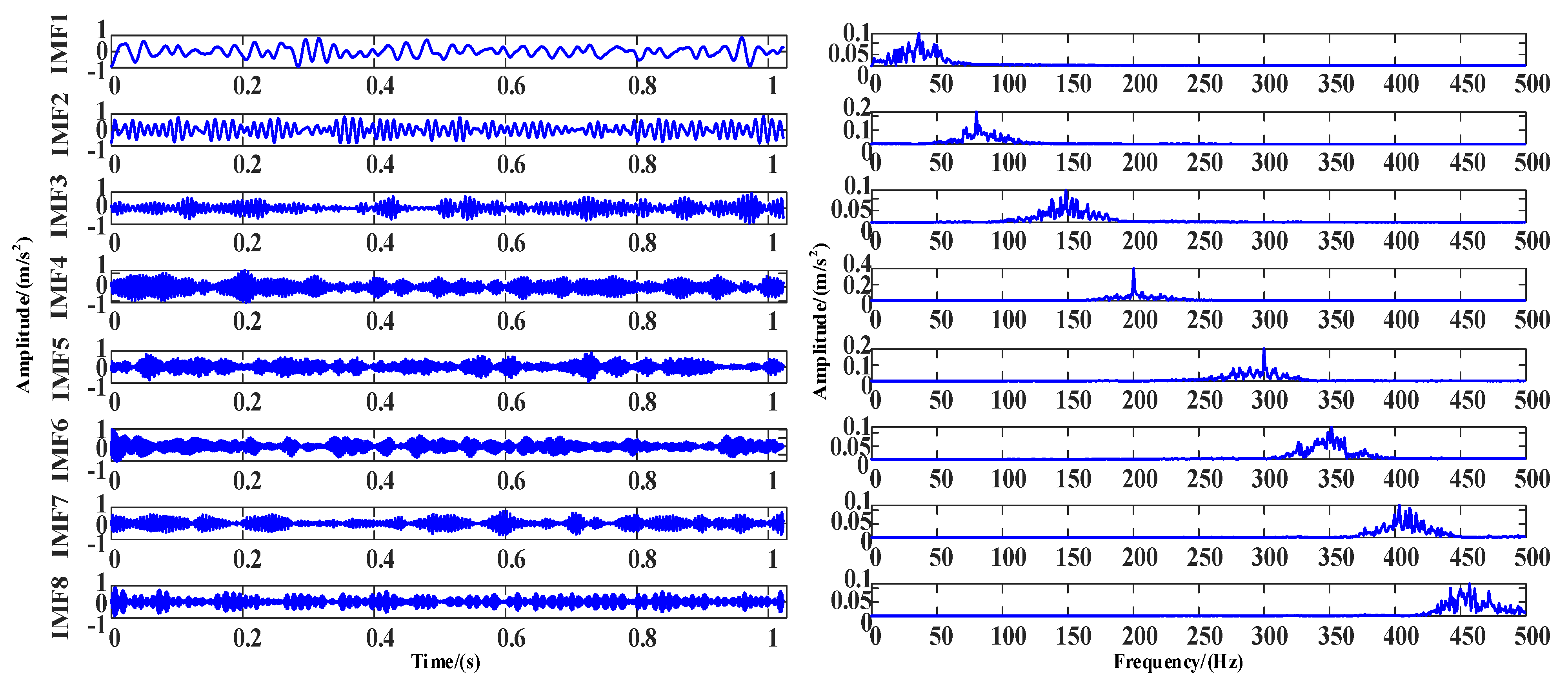
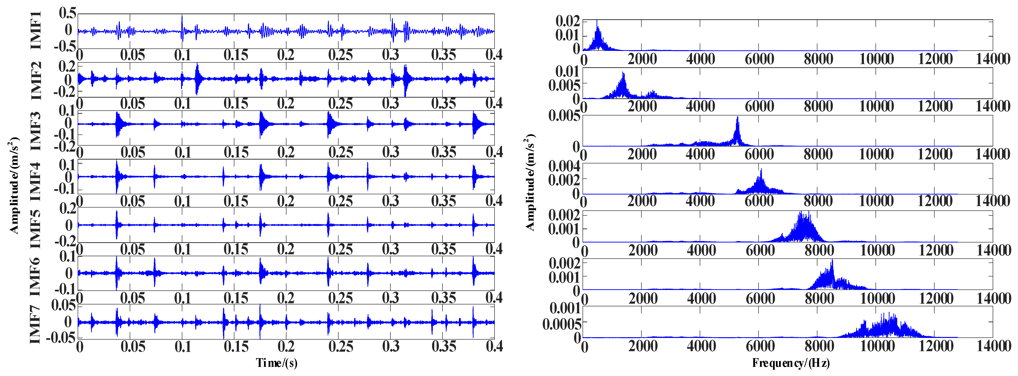
Figure 25.
The time and frequency domain diagram of IMF after WOA-VMD noise decomposition.
Figure 25.
The time and frequency domain diagram of IMF after WOA-VMD noise decomposition.
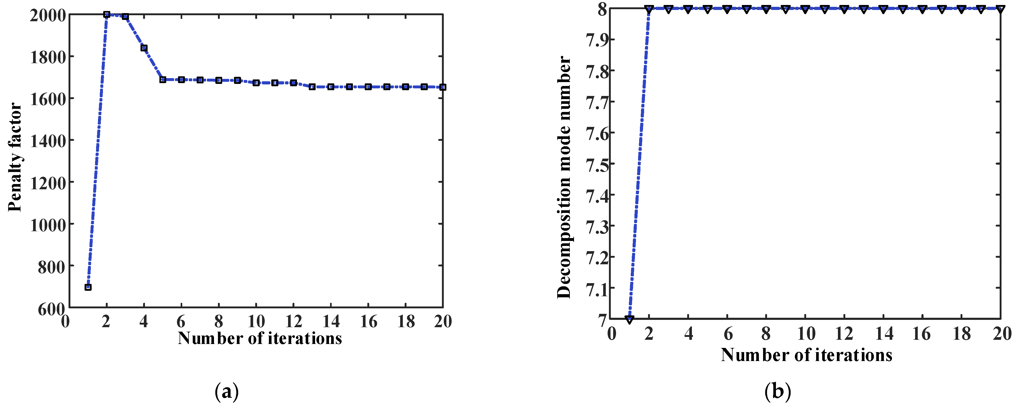
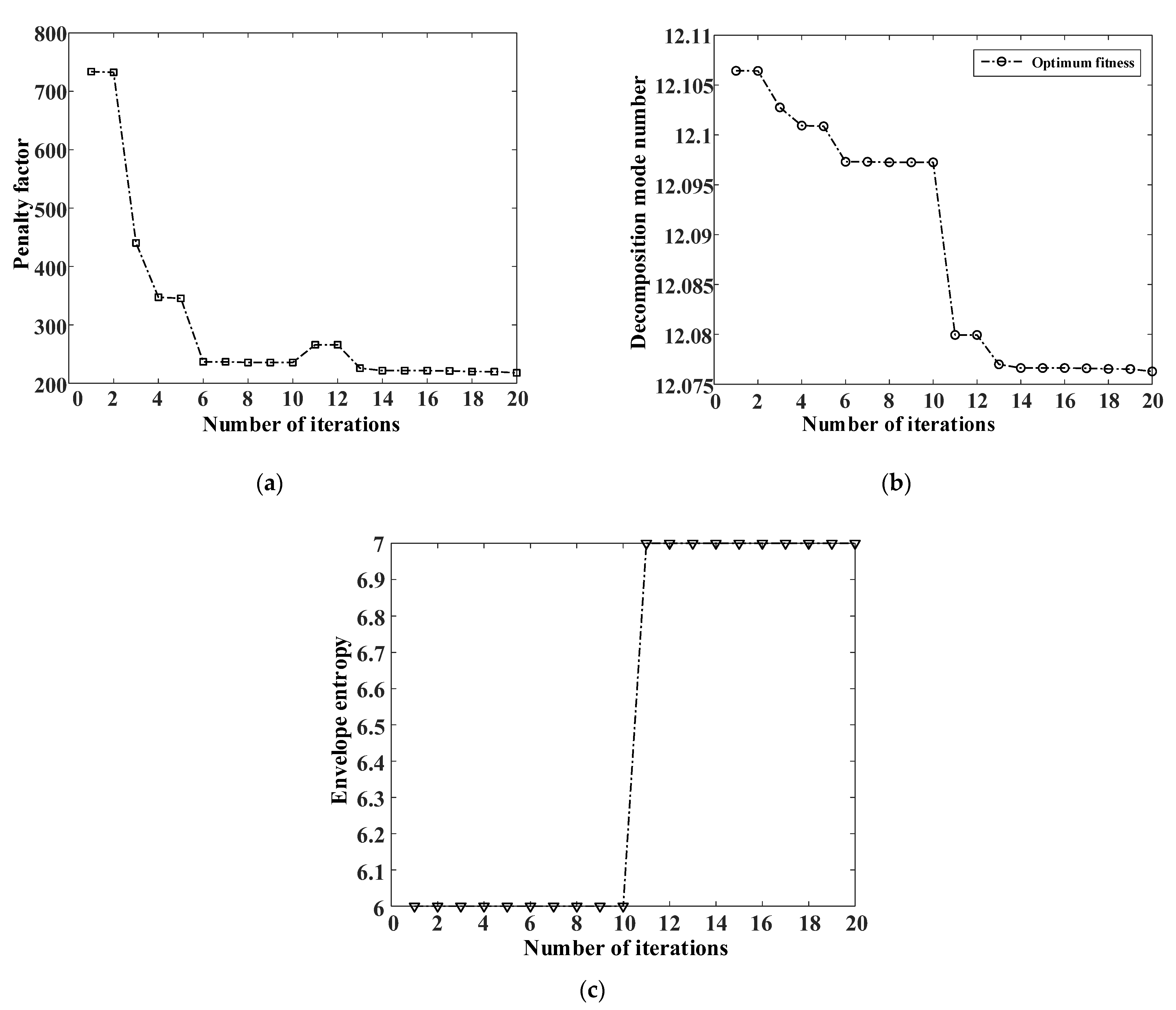
Figure 26.
WOA-VMD iteration curve. (a) Optimization process curve of penalty factor; (b) Optimization process curve of decomposition mode number; (c) Envelope entropy iteration curve of WOA.
Figure 26.
WOA-VMD iteration curve. (a) Optimization process curve of penalty factor; (b) Optimization process curve of decomposition mode number; (c) Envelope entropy iteration curve of WOA.
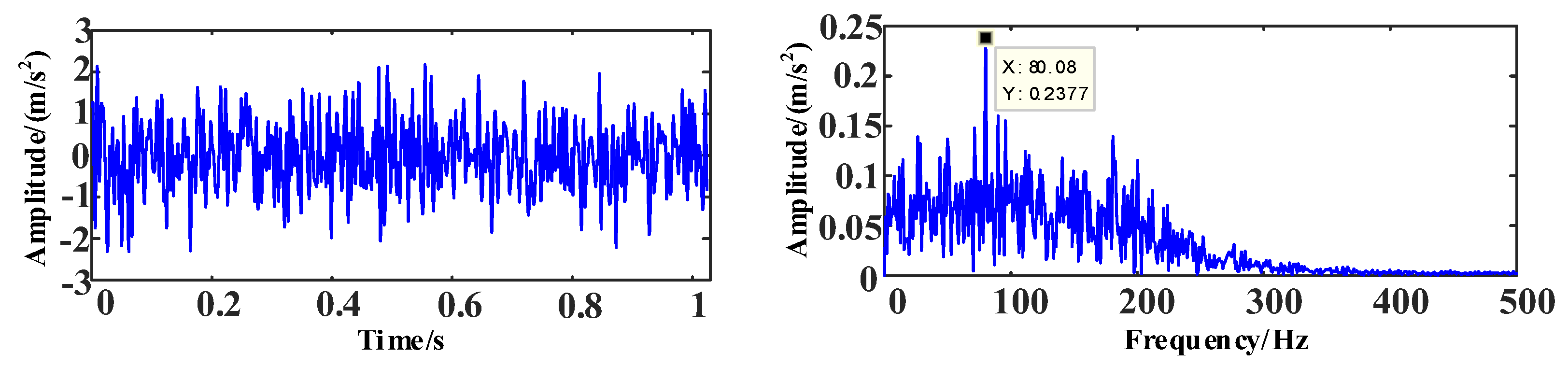
Figure 27.
The time and frequency domain diagrams of the signal after WOA-VMD noise reduction.
Figure 27.
The time and frequency domain diagrams of the signal after WOA-VMD noise reduction.
Figure 28.
Case Western Reserve University bearing Experimental platform.
Figure 28.
Case Western Reserve University bearing Experimental platform.
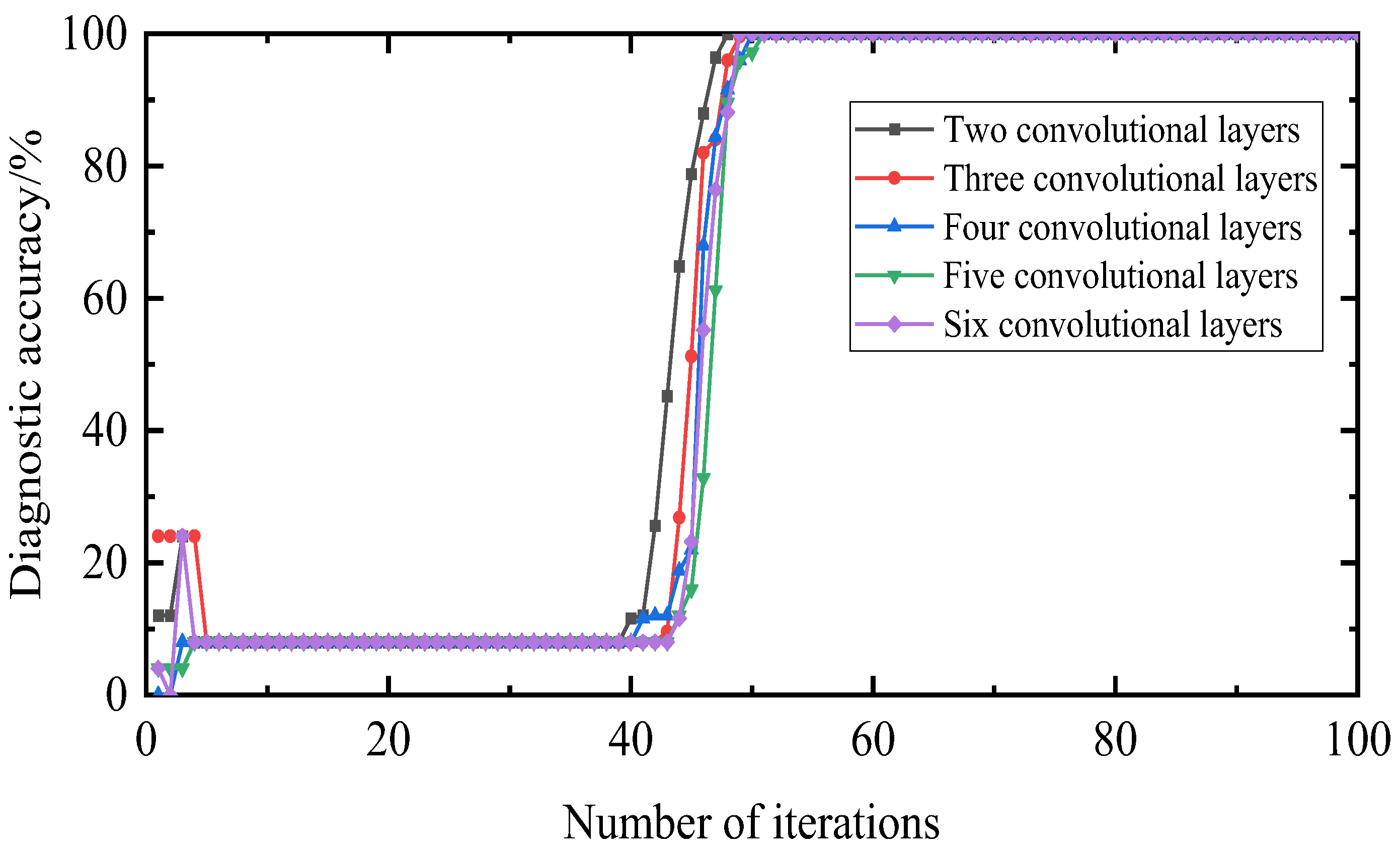
Figure 29.
Diagnostic accuracy under different network layers.
Figure 29.
Diagnostic accuracy under different network layers.
Figure 30.
Loss value under different network layers.
Figure 30.
Loss value under different network layers.
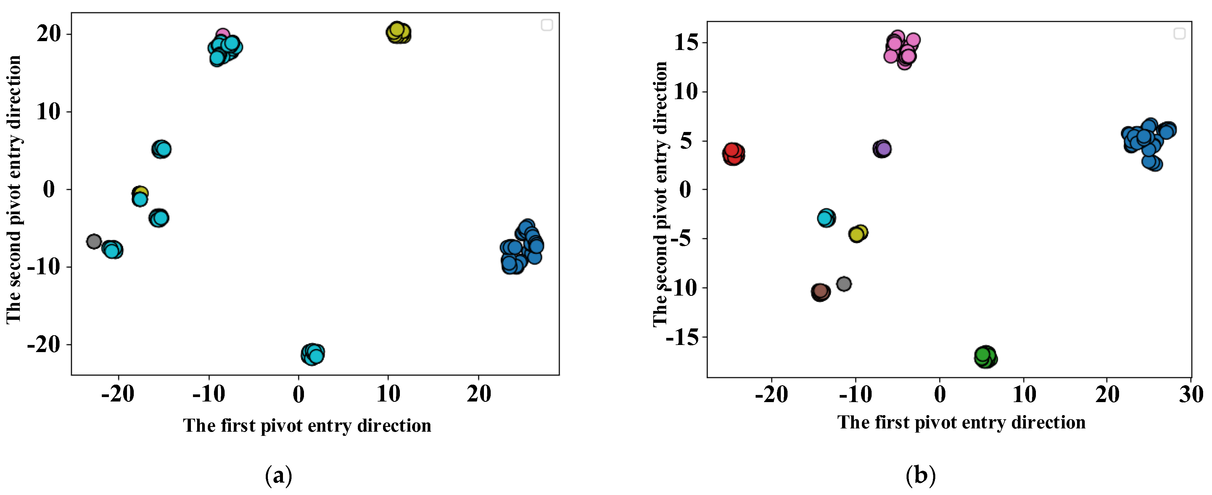
Figure 31.
GAT rolling bearing fault diagnosis model visualization. (a) Initial data set visualization; (b) Visualization of GAT output results.
Figure 31.
GAT rolling bearing fault diagnosis model visualization. (a) Initial data set visualization; (b) Visualization of GAT output results.
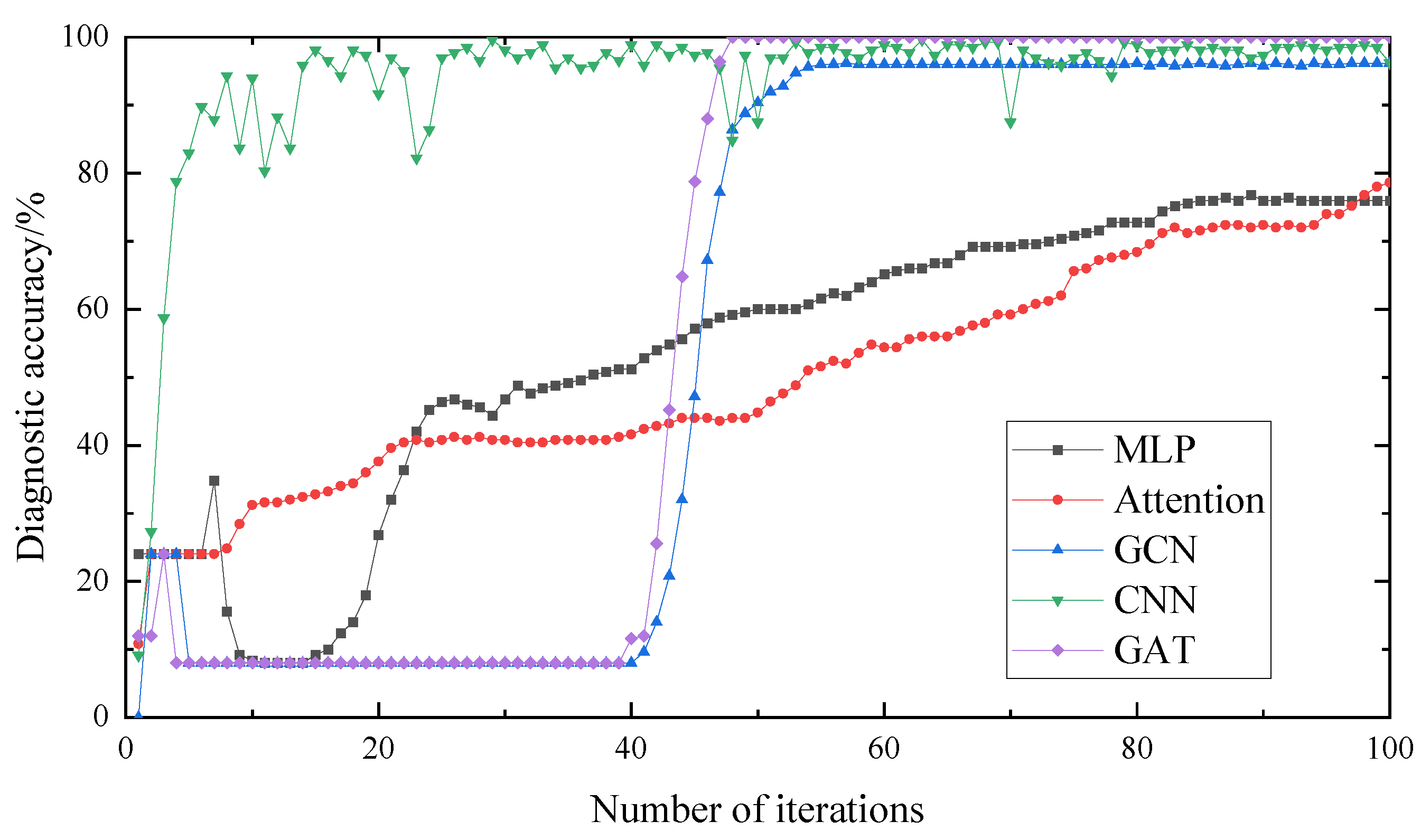
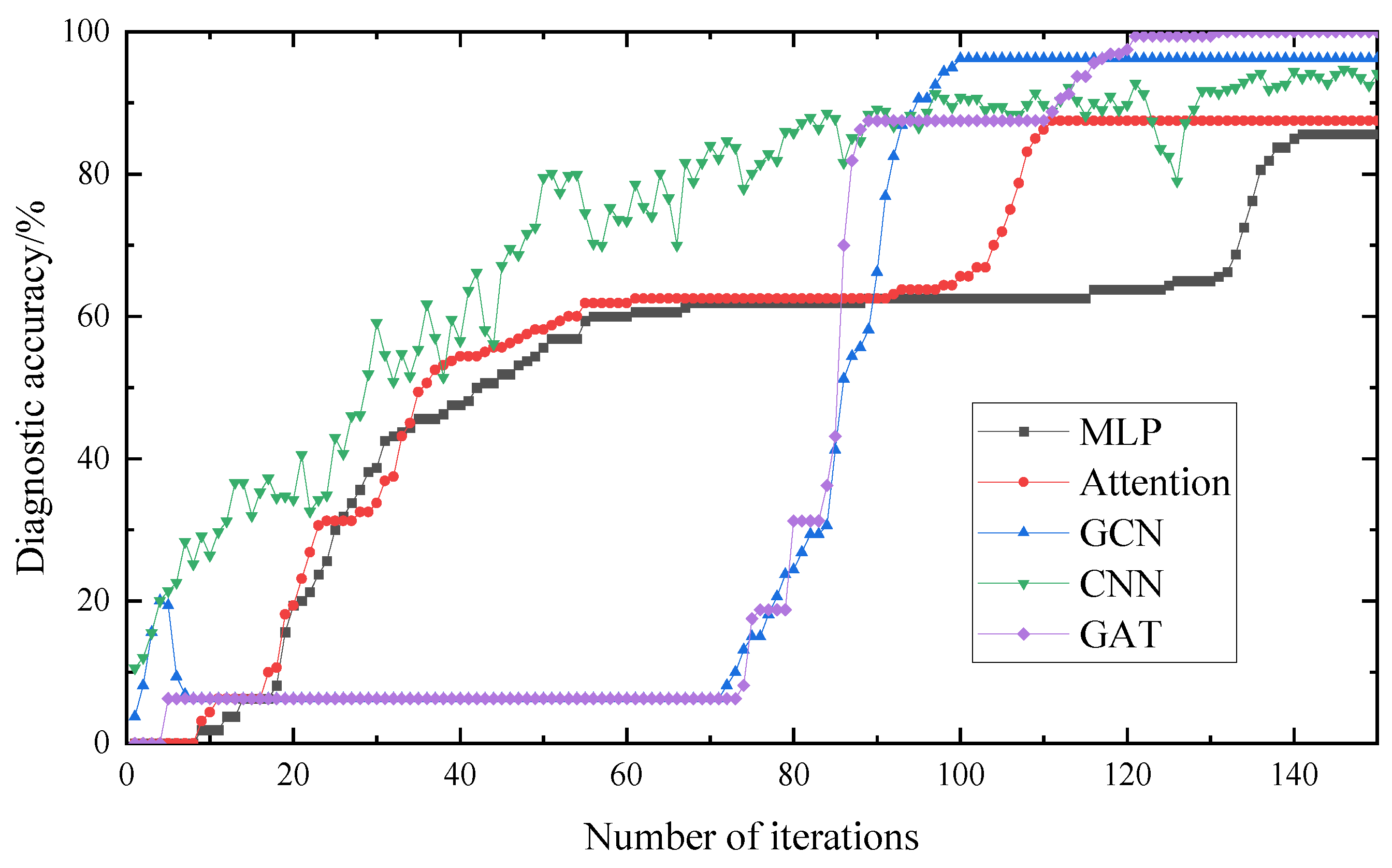
Figure 32.
Diagnostic accuracy of different methods.
Figure 32.
Diagnostic accuracy of different methods.
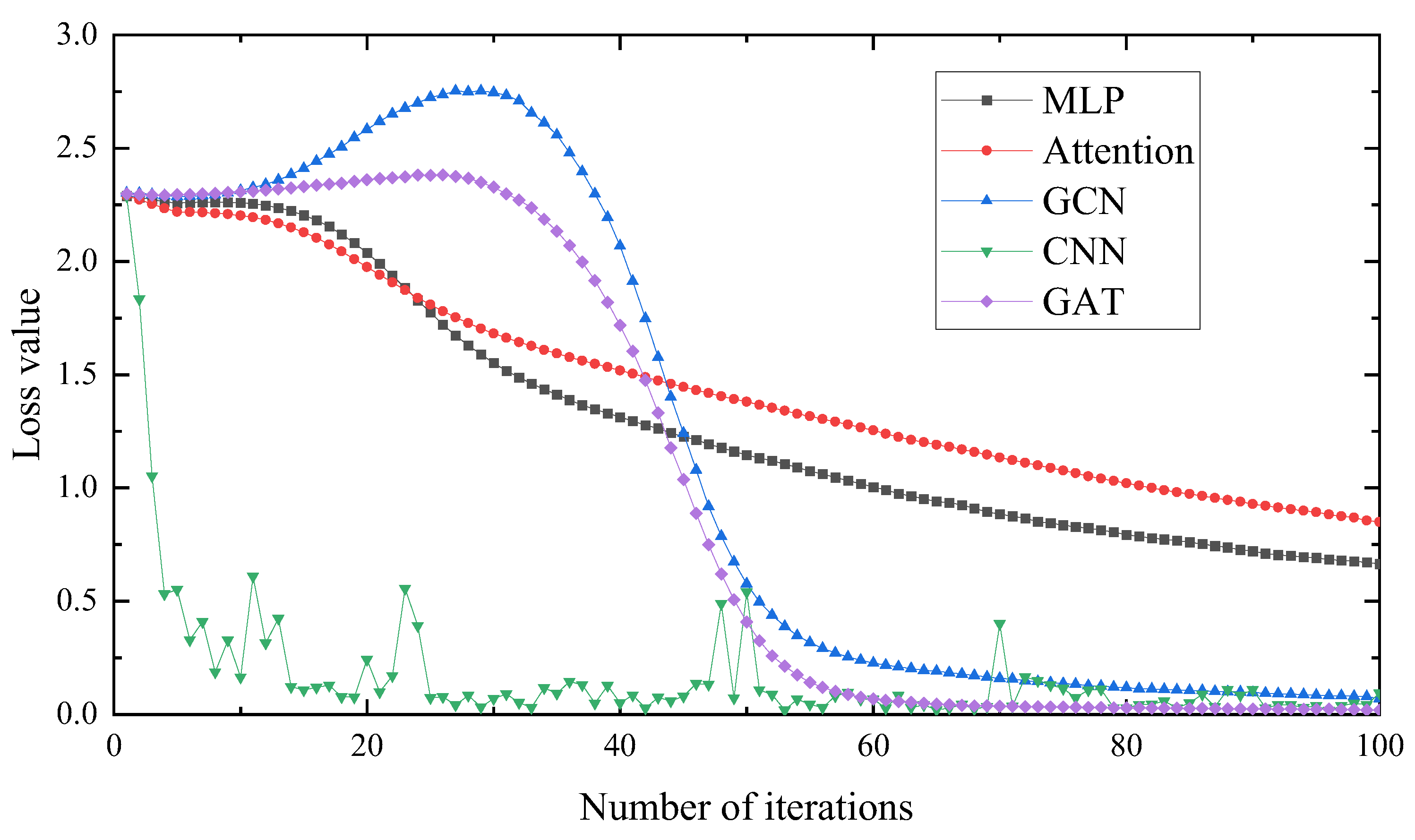
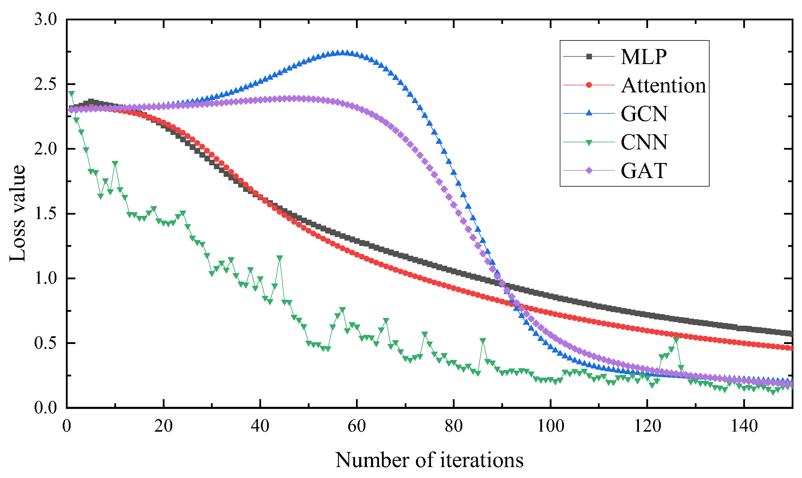
Figure 33.
Loss value of different methods.
Figure 33.
Loss value of different methods.
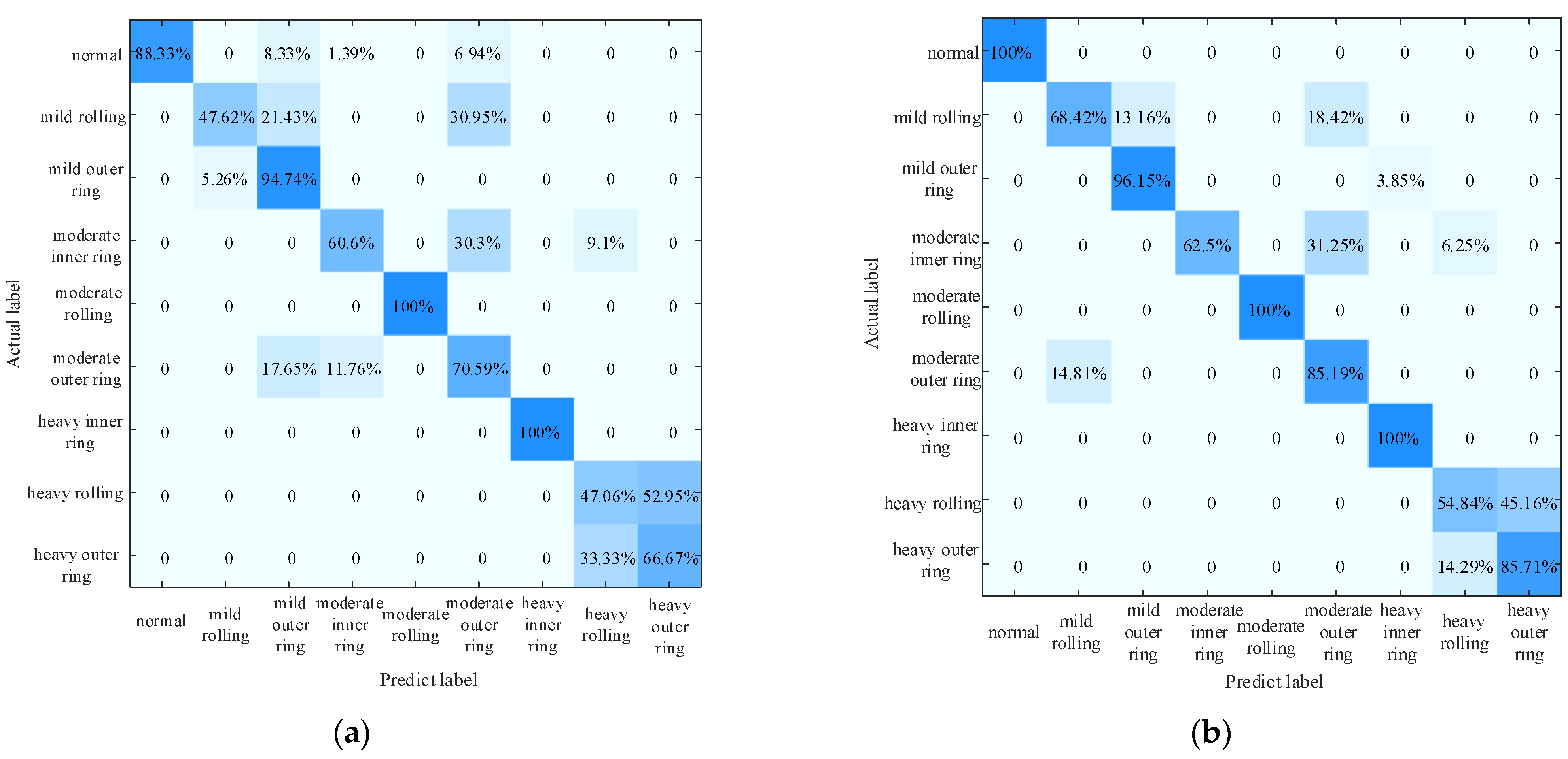
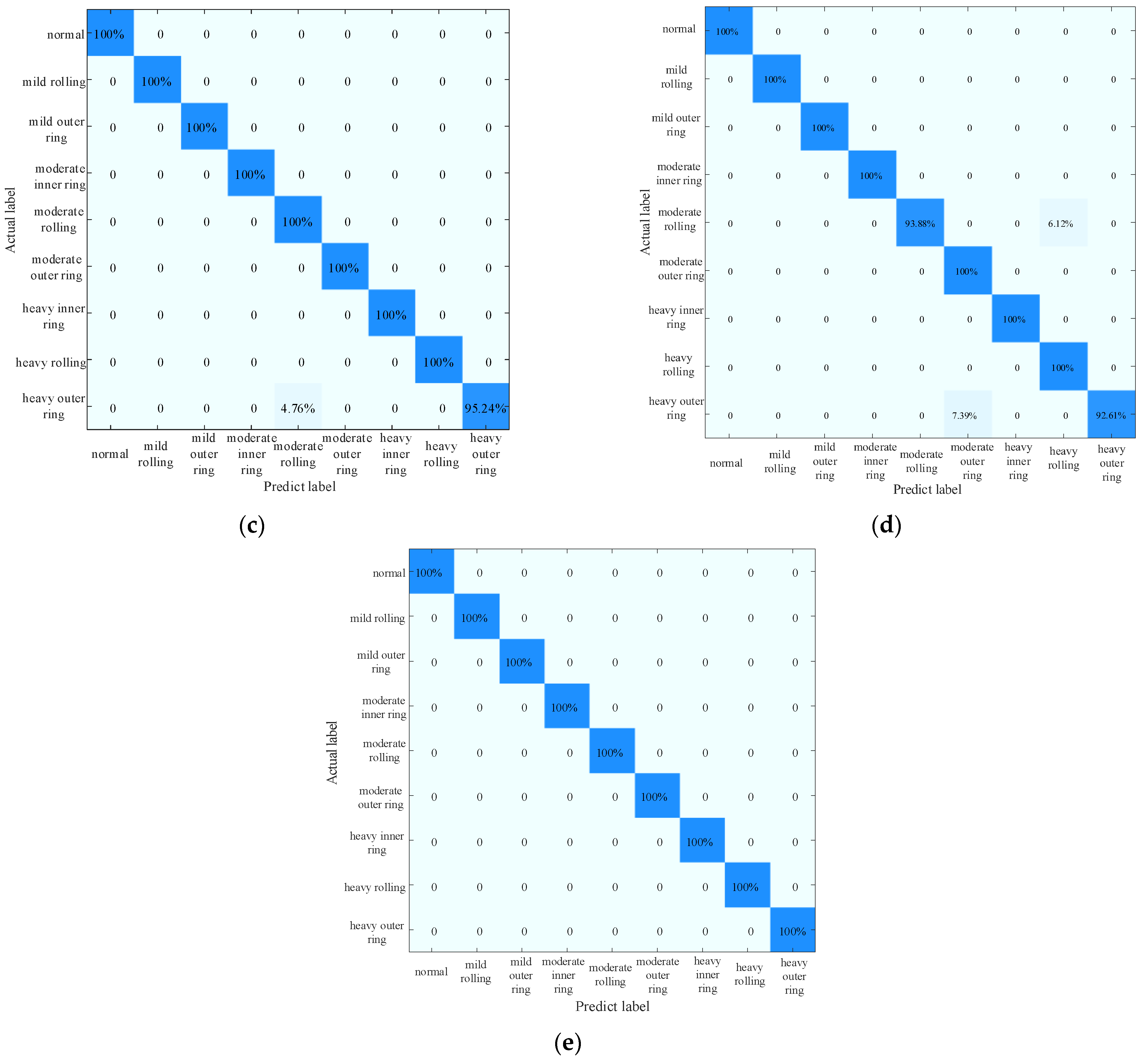
Figure 34.
Confusion matrix of different methods. (a) Attention; (b) MLP; (c) GCN; (d) GCN; (e) GAT.
Figure 34.
Confusion matrix of different methods. (a) Attention; (b) MLP; (c) GCN; (d) GCN; (e) GAT.
Figure 35.
Diagnostic accuracy of different methods.
Figure 35.
Diagnostic accuracy of different methods.
Figure 36.
Loss value of different methods.
Figure 36.
Loss value of different methods.
Table 1.
Correlation discrimination table.
Table 1.
Correlation discrimination table.
| Interrelation | r(xt,xIMF) Coefficient Values |
|---|
| Very weakly correlated or uncorrelated | 0.0–0.2 |
| weakly correlated | 0.2–0.4 |
| Moderate correlation | 0.4–0.6 |
| Strongly related | 0.6–0.8 |
| Extremely strong correlation | 0.8–1.0 |
Table 2.
Whale optimization algorithm parameter setting value.
Table 2.
Whale optimization algorithm parameter setting value.
| Parameter | Values |
|---|
| Population size | 10 |
| Maximum number of iterations | 20 |
| Number of variables | 2 |
| Range of decomposition layers | [100,3] |
| Penalty factor range | [2000,7] |
Table 3.
Correlation coefficient value of each IMF.
Table 3.
Correlation coefficient value of each IMF.
| Mode Component | Correlation Coefficient |
|---|
| IMF1 | 0.5167 |
| IMF2 | 0.8005 |
| IMF3 | 0.4942 |
| IMF4 | 0.7966 |
| IMF5 | 0.7854 |
| IMF6 | 0.6258 |
| IMF7 | 0.4135 |
| IMF8 | 0.4638 |
Table 4.
Comparison of different noise reduction methods under simulation data.
Table 4.
Comparison of different noise reduction methods under simulation data.
| Noise Reduction Algorithms | Root Mean Square Error | Signal to Noise Ratio |
|---|
| EMD noise reduction | 0.738 | 4.018 |
| EEMD noise reduction | 0.780 | 3.958 |
| CEEMD noise reduction | 0.785 | 3.804 |
| GA-VMD noise reduction | 0.702 | 4.112 |
| WOA-VMD noise reduction | 0.213 | 6.912 |
Table 5.
Parameters of the test bench.
Table 5.
Parameters of the test bench.
| Bearing Parameters | Values | Bearing Parameters | Values |
|---|
| Outer ring diameter | 51.99 mm | Inner ring diameter | 25.40 mm |
| Weight | 0.28 kg | Rolling diameter | 7.92 mm |
| Number of rolling elements | 9 | Contact angle | 0° |
| Maximum load (static) | 7830 N | Maximum load (dynamic) | 10,810 kN |
Table 6.
A data set of bearing fault diagnosis experiment.
Table 6.
A data set of bearing fault diagnosis experiment.
| Radial Loading Force | Fault Location | Data Set | Degree of Damage |
|---|
| 0 kg | Inner ring | I_L_0 | mild |
| I_M_0 | moderate |
| I_H_0 | heavy |
| Outer ring | O_L_0 | mild |
| O_M_0 | moderate |
| O_H_0 | heavy |
| Rolling ball | B_L_0 | mild |
| B_M_0 | moderate |
| B_H_0 | heavy |
| 100 kg | Inner ring | I_L_100 | mild |
| I_M_100 | moderate |
| I_H_100 | heavy |
| Outer ring | O_L_100 | mild |
| O_M_100 | moderate |
| O_H_100 | heavy |
| Rolling ball | B_L_100 | mild |
| B_M_100 | moderate |
| B_H_100 | heavy |
| 200 kg | Inner ring | I_L_200 | mild |
| I_M_200 | moderate |
| I_H_200 | heavy |
| Outer ring | O_L_200 | mild |
| O_M_200 | moderate |
| O_H_200 | heavy |
| Rolling ball | B_L_200 | mild |
| B_M_200 | moderate |
| B_H_200 | heavy |
Table 7.
Correlation coefficient value of each IMF.
Table 7.
Correlation coefficient value of each IMF.
| Mode Component | Correlation Coefficient |
|---|
| IMF1 | 0.8262 |
| IMF2 | 0.6075 |
| IMF3 | 0.2630 |
| IMF4 | 0.2203 |
| IMF5 | 0.2069 |
| IMF6 | 0.1824 |
| IMF7 | 0.1065 |
Table 8.
Experimental parameter settings for different fault states.
Table 8.
Experimental parameter settings for different fault states.
| Experiment Number | Fault Size | Fault Location | Location of Collection End |
|---|
| No. 1 | 0 | Normal | |
| No. 2 | 0.007 inch | Inner ring fault | 12 k Driving end |
| No. 3 | 0.007 inch | Outer ring fault | 12 k Driving end |
| No. 4 | 0.007 inch | Rolling fault | 12 k Driving end |
| No. 5 | 0.014 inch | Inner ring fault | 12 k Fan end |
| No. 6 | 0.014 inch | Outer ring fault | 12 k Fan end |
| No. 7 | 0.014 inch | Rolling fault | 12 k Fan end |
| No. 8 | 0.021 inch | Inner ring fault | 48 k Driving end |
| No. 9 | 0.021 inch | Outer ring fault | 48 k Driving end |
| No. 10 | 0.021 inch | Rolling fault | 48 k Driving end |
Table 9.
GAT model parameters.
Table 9.
GAT model parameters.
| Parameter Name | Value | Parameter Name | Value |
|---|
| Number of the training set sample groups | 97 | Node deactivation rate | 0.2 |
| Number of sample groups of verification set | 25 | Second fully connected layer | [1024,1024] |
| Number of test set sample groups | 122 | Batch normalization | 1024 |
| Convolutional kernel of the first layer | [2048,2048] | Loss function | Cross-entropy loss function |
| Convolutional kernel of the second layer | [2048,2048] | Optimizer | Stochastic gradient descent |
| Activation function of the first layer | Relu | Training times | 100 |
| Activation function of the second layer | Relu | Batch size | 64 |
| First fully connected layer | [2048,1024] | Learning rate | 0.01 |
Table 10.
Diagnostic accuracy of different graph convolution kernel size.
Table 10.
Diagnostic accuracy of different graph convolution kernel size.
| Size | | | |
|---|
| Accuracy | 90.40% | 96.85% | 92.81% |
| Time/s | 42.25 | 61.58 | 120.54 |
Table 11.
Diagnostic accuracy of test sets of different algorithms.
Table 11.
Diagnostic accuracy of test sets of different algorithms.
| MLP | Attention | GCN | CNN | GAT |
|---|
| 82.40% | 70.8% | 99.6% | 98.32% | 100% |
Table 12.
The diagnostic precision of test sets of different algorithms.
Table 12.
The diagnostic precision of test sets of different algorithms.
| | MLP | Attention | GCN | CNN | GAT |
|---|
| normal | 100% | 83.30% | 100% | 97.19% | 100% |
| mild rolling | 68.42% | 47.62% | 100% | 96.16% | 100% |
| mild outer ring | 96.15% | 94.74% | 100% | 100% | 100% |
| moderate inner ring | 62.50% | 60.60% | 100% | 95.37% | 100% |
| moderate rolling | 100% | 100% | 100% | 88.06% | 100% |
| moderate outer ring | 85.19% | 70.59% | 100% | 96.42% | 100% |
| heavy inner ring | 100% | 100% | 100% | 97.42% | 100% |
| heavy rolling | 54.84% | 47.06% | 100% | 100% | 100% |
| heavy outer ring | 85.71% | 66.67% | 95.24% | 98.25% | 100% |
Table 13.
Diagnostic accuracy of test sets of different algorithms.
Table 13.
Diagnostic accuracy of test sets of different algorithms.
| MLP | Attention | GCN | GCN | GAT |
|---|
| 85.62% | 87.25% | 96.25% | 94.12% | 100% |
Table 14.
Diagnostic accuracy of test sets of different algorithms.
Table 14.
Diagnostic accuracy of test sets of different algorithms.
| | MLP | Attention | GCN | CNN | GAT |
|---|
| normal | 100% | 100% | 100% | 100% | 100% |
| mild rolling | 0% | 0% | 0% | 100% | 100% |
| mild outer ring | 100% | 100% | 100% | 80% | 100% |
| moderate inner ring | 100% | 100% | 100% | 50% | 100% |
| moderate rolling | 100% | 100% | 100% | 100% | 100% |
| moderate outer ring | 100% | 100% | 100% | 90% | 100% |
| heavy inner ring | 100% | 100% | 100% | 100% | 100% |
| heavy rolling | 100% | 100% | 100% | 100% | 100% |
| heavy outer ring | 0% | 0% | 100% | 100% | 100% |


