

Advancing Continuous Distribution Generation: An Exponentiated Odds Ratio Generator Approach


Abstract
1. Introduction
2. The New Generator Based on Odds Ratio
3. The Type 2 Gumbel Weibull-G Family of Distributions
3.1. Expansion of the pdf
3.2. Hazard Rate and Quantile Functions
3.2.1. Hazard Rate and Quantile Functions
3.2.2. Quantile Function
3.3. Moments, Incomplete Moments, and Generating Functions
3.3.1. Moments
3.3.2. Incomplete Moments, Conditional Moments, and Moment Generating Function
3.4. Rényi Entropy
3.5. Order Statistics
3.6. Stochastic Ordering
4. Methods of Estimation
4.1. Maximum Likelihood Estimation
4.2. Least Square and Weighted Least Square Estimation
4.3. Maximum Product Spacing Approach of Estimation
4.4. Cramér–Von Mises Approach of Estimation
4.5. Anderson and Darling Approach of Estimation
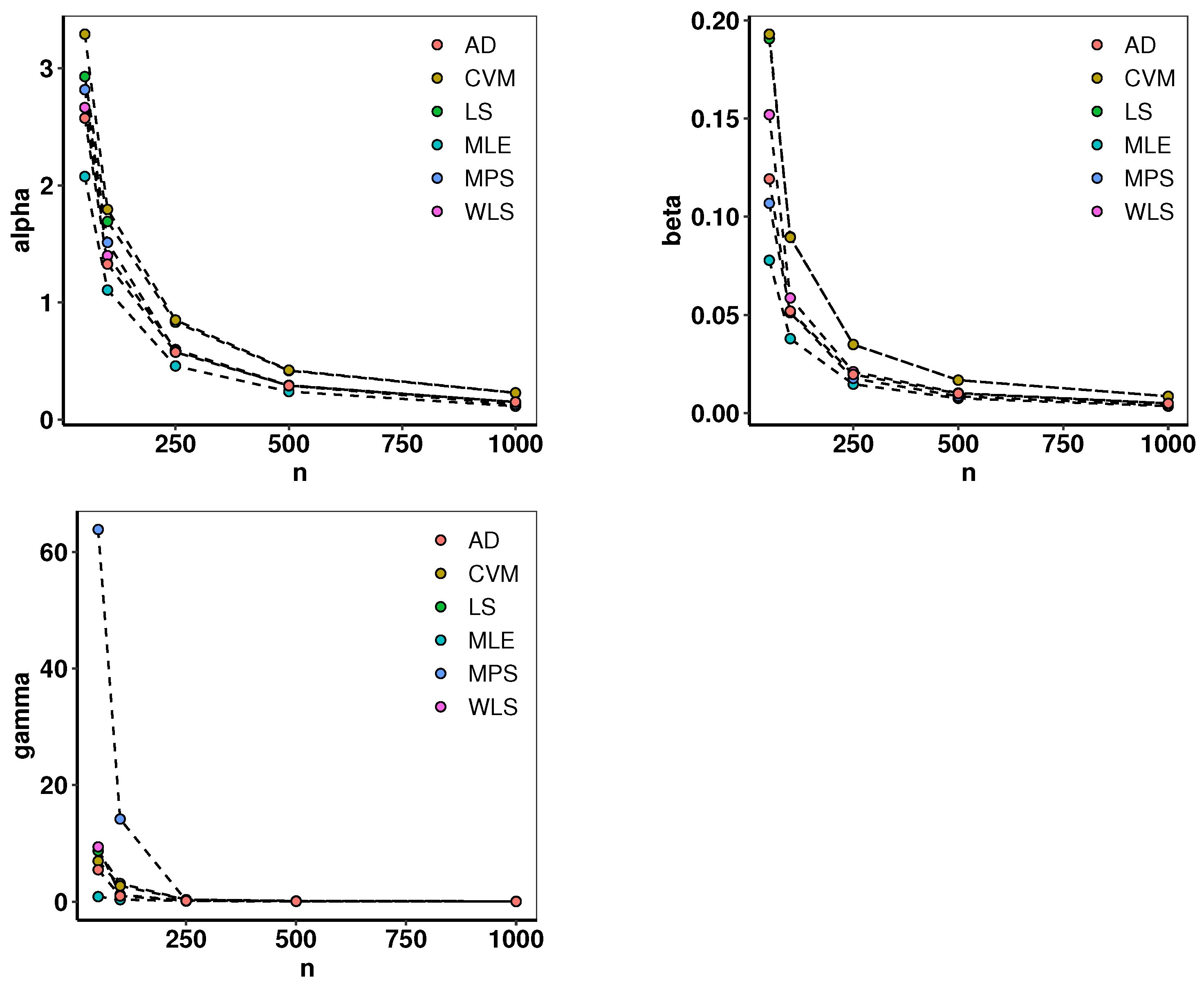
4.6. Simulation and Estimation
5. Special Cases
5.1. Type 2 Gumbel Weibull–Exponential (T2GWE) Distribution
5.1.1. cdf and pdf of the T2GWE Distribution
5.1.2. Hazard Rate and Quantile Functions
5.2. Type 2 Gumbel Weibull–Uniform (T2GWU) Distribution
5.2.1. cdf and pdf of the T2GWU Distribution
5.2.2. Hazard Rate and Quantile Functions
5.3. Type 2 Gumbel Weibull–Pareto (T2GWP) Distribution
5.3.1. cdf and pdf of the T2GWP Distribution
5.3.2. Hazard Rate and Quantile Functions
6. Applications
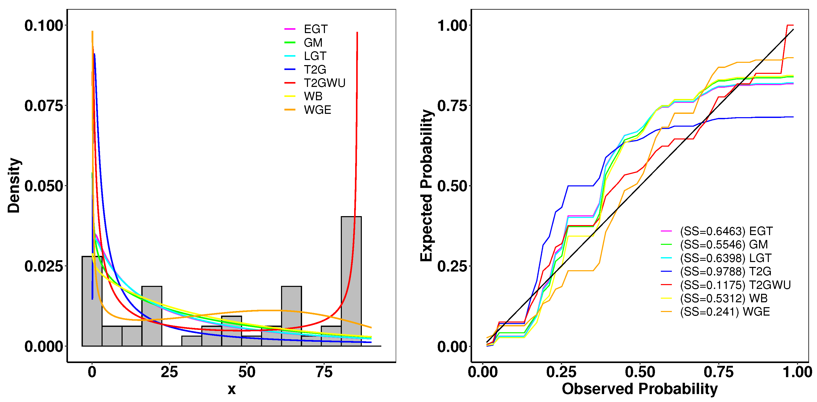
6.1. Aarset Data
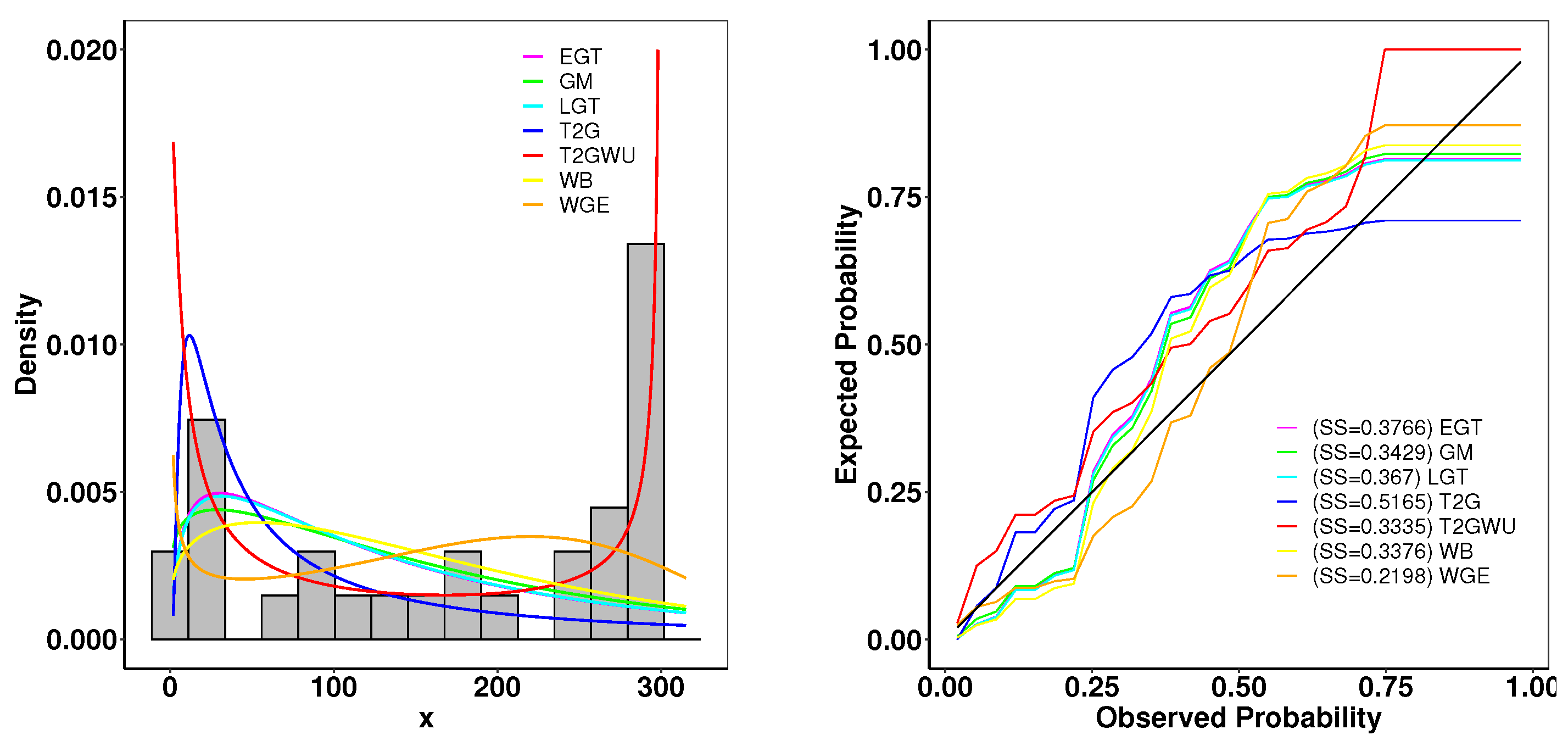
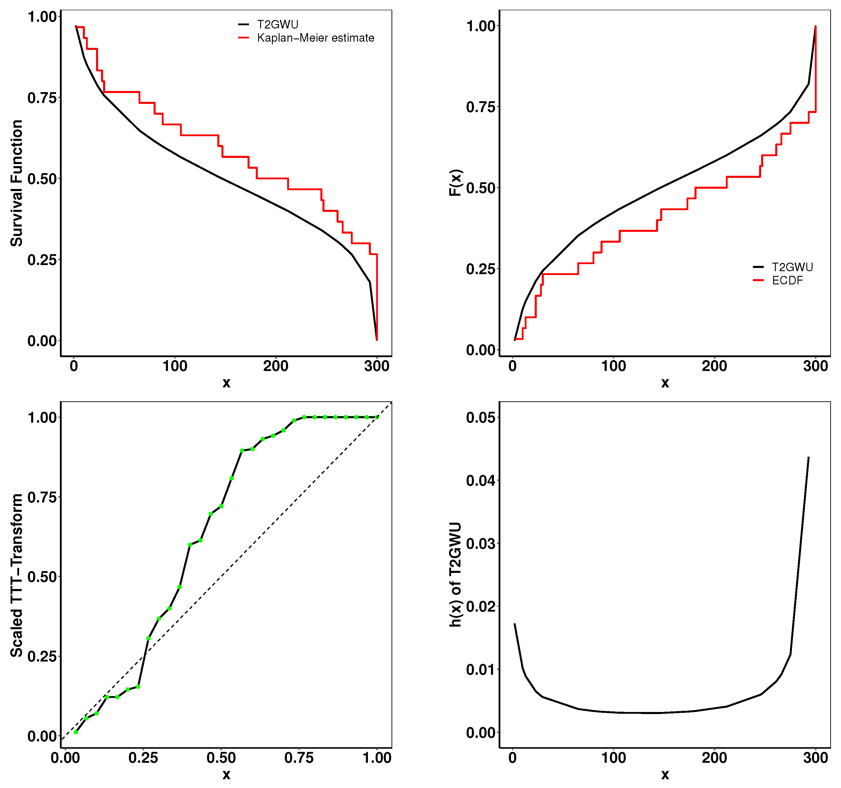
6.2. Meeker and Escobar Data
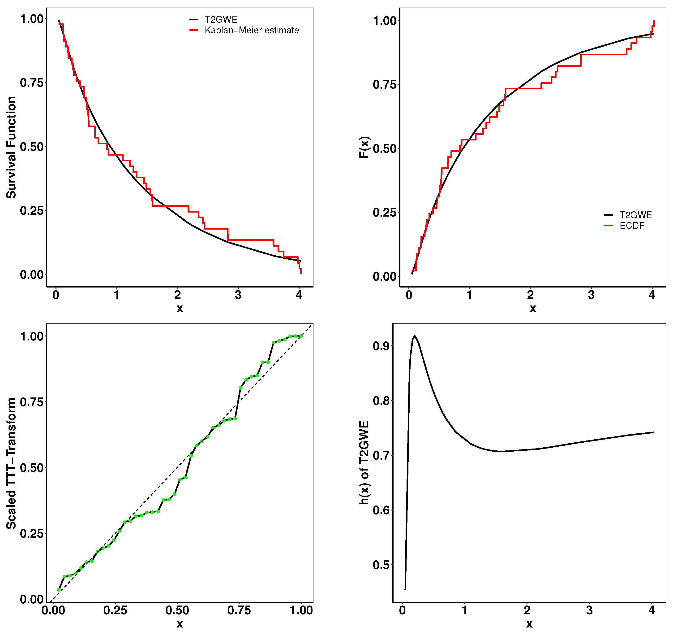
6.3. Chemotherapy Data
- Goodness-of-Fit Analysis: Across all datasets, the proposed distributions demonstrate superior performance compared to existing models. This is evidenced by their lower goodness-of-fit statistics, including -2log-likelihood statistic, , , AIC, BIC, CAIC, HQIC, and K-S and its higher p-values. These metrics confirm the robustness of the proposed distributions in capturing complex data patterns.
- Empirical and Theoretical Fits: The fitted densities closely resemble the empirical histograms and expected probability plots, indicating a strong fit. Additionally, survival curves (Kaplan–Meier estimates) and cumulative distribution functions align well with the theoretical models, supporting the applicability of the proposed family to survival analysis.
- Hazard Rate Characteristics: The total time on test (TTT) and hazard rate plots highlight the capability of the proposed distributions to model non-monotonic hazard rate structures, such as bathtub-shaped curves, which are often challenging for traditional distributions.
7. Conclusions
Author Contributions
Funding
Data Availability Statement
Acknowledgments
Conflicts of Interest
Abbreviations
| T2GWG | The Type 2 Gumbel Weibull-G |
| cdf | cumulative distribution function |
| probability density function | |
| hrf | hazard rate function |
| Exp-G | exponentiated-G |
| EGT | Exponentiated Gumbel Type 2 |
| WGE | Weibull Generalized Exponential |
| LGT | Lomax Gumbel Type 2 |
| T2G | Type 2 Gumbel |
| EWL | Exponentiated Weibull–logistic distribution |
| MLE | maximum likelihood estimate |
| MPS | maximum product spacing estimate |
| LS | least square estimate |
| WLS | weighted least square estimate |
| CVM | Cramér–von Mises estimate |
| AD | Anderson and Darling estimate |
| T2GWE | Type 2 Gumbel Weibull–exponential |
| T2GWU | Type 2 Gumbel Weibull–uniform |
| T2GWP | Type 2 Gumbel Weibull–Pareto |
| AIC | Akaike Information Criterion |
| CAIC | Consistent Akaike Information Criterion |
| BIC | Bayesian Information Criterion |
| HQIC | Hannan–Quinn Criterion |
| Cramér–von Mises statistic | |
| Anderson–Darling statistic | |
| K-S | Kolmogorov–Smirnov statistic |
| ECDF | empirical cumulative distribution function |
| TTT | total time on test |
| K-M | Kaplan–Meier |
Appendix A. The First Derivatives of H
Appendix B. Distributions Used in the Application Section
- Exponentiated Gumbel Type 2 Distribution:
- Weibull Generalized Exponential Distribution:
- Lomax Gumbel Type 2 Distribution:
- Type 2 Gumbel Distribution:
- Exponentiated Weibull–Logistic Distribution:
References
- Rodríguez González, C.A.; Rodríguez-Pérez, A.M.; López, R.; Hernández-Torres, J.A.; Caparrós-Mancera, J.J. Sensitivity Analysis in Mean Annual Sediment Yield Modeling with Respect to Rainfall Probability Distribution Functions. Land 2023, 12, 35. [Google Scholar] [CrossRef]
- Jiang, S.H.; Liu, X.; Wang, Z.Z.; Li, D.Q.; Huang, J. Efficient sampling of the irregular probability distributions of geotechnical parameters for reliability analysis. Struct. Saf. 2023, 101, 102309. [Google Scholar] [CrossRef]
- Klein, J.P.; Moeschberger, M.L. Survival Analysis: Techniques for Censored and Truncated Data; Springer Science & Business Media: New York, NY, USA, 2006. [Google Scholar]
- Bain, L.J.; Engelhardt, M. Reliability Test Plans for One-Shot Devices Based on Repeated Samples. J. Qual. Technol. 1991, 23, 304–311. [Google Scholar] [CrossRef]
- Cooray, K. Generalization of the Weibull distribution: The odd Weibull family. Stat. Model. 2006, 6, 265–277. [Google Scholar] [CrossRef]
- Bourguignon, M.; Silva, R.B.; Cordeiro, G.M. The Weibull-G family of probability distributions. J. Data Sci. 2014, 12, 53–68. [Google Scholar] [CrossRef]
- Pu, S.; Oluyede, B.O.; Qiu, Y.; Linder, D. A Generalized Class of Exponentiated Modified Weibull Distribution with Applications. J. Data Sci. 2016, 14, 585–613. [Google Scholar] [CrossRef]
- Oluyede, B.; Pu, S.; Makubate, B.; Qiu, Y. The gamma-Weibull-G Family of distributions with applications. Austrian J. Stat. 2018, 47, 45–76. [Google Scholar] [CrossRef]
- Oluyede, B.; Moakofi, T. The Gamma-Topp-Leone-Type II-Exponentiated Half Logistic-G Family of Distributions with Applications. Stats 2023, 6, 706–733. [Google Scholar] [CrossRef]
- Shama, M.S.; Alharthi, A.S.; Almulhim, F.A.; Gemeay, A.M.; Meraou, M.A.; Mustafa, M.S.; Hussam, E.; Aljohani, H.M. Modified generalized Weibull distribution: Theory and applications. Sci. Rep. 2023, 13, 12828. [Google Scholar] [CrossRef]
- Emam, W.; Tashkandy, Y. Modeling the Amount of Carbon Dioxide Emissions Application: New Modified Alpha Power Weibull-X Family of Distributions. Symmetry 2023, 15, 366. [Google Scholar] [CrossRef]
- Gabanakgosi, M.; Oluyede, B. The Topp-Leone type II exponentiated half logistic-G family of distributions with applications. Int. J. Math. Oper. Res. 2023, 25, 85–117. [Google Scholar] [CrossRef]
- Sun, J.; Kong, M.; Pal, S. The Modified-Half-Normal distribution: Properties and an efficient sampling scheme. Commun. -Stat.-Theory Methods 2023, 52, 1591–1613. [Google Scholar] [CrossRef]
- Guptha, R.C.S.; Maruthan, S.K. A New Generalization of Power Lindley Distribution and Its Applications. Thail. Stat. 2023, 21, 196–208. [Google Scholar]
- Pu, S.; Moakofi, T.; Oluyede, B. The Ristić–Balakrishnan–Topp–Leone–Gompertz-G Family of Distributions with Applications. J. Stat. Theory Appl. 2023, 22, 116–150. [Google Scholar] [CrossRef]
- Kajuru, J.; Dikko, H.; Mohammed, A.; Fulatan, A. odd Gompertz-G Family of Distribution, its Properties and Applications. Fudma J. Sci. 2023, 7, 351–358. [Google Scholar] [CrossRef]
- Osagie, S.A.; Uyi, S.; Osemwenkhae, J.E. The Inverse Burr-Generalized Family of Distributions: Theory and Applications. Earthline J. Math. Sci. 2023, 13, 313–351. [Google Scholar] [CrossRef]
- Marasigan, A.E. A New Extension of the Inverse Paralogistic Distribution using Gamma Generator with Application. Mindanao J. Sci. Technol. 2023, 21, 59–80. [Google Scholar] [CrossRef]
- Azimi, R.; Esmailian, M. A new generalization of Nadarajah-Haghighi distribution with application to cancer and COVID-19 deaths data. Math. Slovaca 2023, 73, 221–244. [Google Scholar]
- Scheidegger, A.; Leitao, J.P.; Scholten, L. Statistical failure models for water distribution pipes–A review from a unified perspective. Water Res. 2015, 83, 237–247. [Google Scholar] [CrossRef]
- Romaniuk, M.; Hryniewicz, O. Estimation of maintenance costs of a pipeline for a U-shaped hazard rate function in the imprecise setting. Eksploat. Niezawodn. 2020, 22, 352–362. [Google Scholar] [CrossRef]
- Chachra, A.; Kumar, A.; Ram, M. A Markovian approach to reliability estimation of series-parallel system with Fermatean fuzzy sets. Comput. Ind. Eng. 2024, 190, 110081. [Google Scholar] [CrossRef]
- Kleinbaum, D.G.; Klein, M. Survival Analysis a Self-Learning Text; Springer: New York, NY, USA, 1996. [Google Scholar]
- Tsiatis, A.A.; Davidian, M.; Holloway, S.T. Estimation of the odds ratio in a proportional odds model with censored time-lagged outcome in a randomized clinical trial. Biometrics 2023, 79, 975–987. [Google Scholar] [CrossRef] [PubMed]
- VanderWeele, T.J. Optimal approximate conversions of odds ratios and hazard ratios to risk ratios. Biometrics 2020, 76, 746–752. [Google Scholar] [CrossRef] [PubMed]
- Penner, C.G.; Gerardy, B.; Ryan, R.; Williams, M. The Odds Ratio Product (An Objective Sleep Depth Measure): Normal Values, Repeatability, and Change With CPAP in Patients With OSA: The Odds Ratio Product. J. Clin. Sleep Med. 2019, 15, 1155–1163. [Google Scholar] [CrossRef]
- Alzaatreh, A.; Carl, L.; Felix, F. A new method for generating families of continuous distributions. Metron 2013, 71, 63–79. [Google Scholar] [CrossRef]
- Yang, H.; Huang, M.; Chen, X.; He, Z.; Pu, S. Enhanced Real-Life Data Modeling with the Modified Burr III Odds Ratio–G Distribution. Axioms 2024, 13, 401. [Google Scholar] [CrossRef]
- Roy, S.S.; Knehr, H.; McGurk, D.; Chen, X.; Cohen, A.; Pu, S. The Lomax-Exponentiated Odds Ratio–G Distribution and Its Applications. Mathematics 2024, 12, 1578. [Google Scholar] [CrossRef]
- Al-Moisheer, A.; Elbatal, I.; Almutiry, W.; Elgarhy, M. Odd inverse power generalized Weibull generated family of distributions: Properties and applications. Math. Probl. Eng. 2021, 2021, 5082192. [Google Scholar] [CrossRef]
- ul Haq, M.A.; Elgarhy, M. The Odd Frèchet-G family of probability distributions. J. Stat. Appl. Probab. 2018, 7, 189–203. [Google Scholar] [CrossRef]
- Rényi, A. On measures of entropy and information. In Proceedings of the 4th Berkeley Symposium on Mathematical Statistics and Probability, Berkeley, CA, USA, 20 June–30 July 1961; Volume 1, pp. 547–561. [Google Scholar]
- Szekli, R. Stochastic Ordering and Dependence in Applied Probability; Springer Science & Business Media: New York, NY, USA, 2012; Volume 97. [Google Scholar]
- Cheng, R.C.H.; Amin, N.A.K. Estimating Parameters in Continuous Univariate Distributions with a Shifted Origin. J. R. Stat. Soc. Ser. B Methodol. 1983, 45, 394–403. [Google Scholar] [CrossRef]
- MacDonald, P.D.M. Comment on “An Estimation Procedure for Mixtures of Distributions” by Choi and Bulgren. J. R. Stat. Soc. Ser. B Methodol. 1971, 33, 326–329. [Google Scholar] [CrossRef]
- Anderson, T.W.; Darling, D.A. A test of goodness of fit. J. Am. Stat. Assoc. 1954, 49, 765–769. [Google Scholar] [CrossRef]
- Okorie, I.E.; Akpanta, A.; Ohakwe, J. The exponentiated Gumbel type-2 distribution: Properties and application. Int. J. Math. Math. Sci. 2016, 2016, 5898356. [Google Scholar] [CrossRef]
- Mustafa, A.; El-Desouky, B.S.; AL-Garash, S. Weibull generalized exponential distribution. arXiv 2016, arXiv:1606.07378. [Google Scholar]
- Adeyemi, A.O.; Adeleke, I.A.; Akarawak, E.E. Lomax gumbel type two distributions with applications to lifetime data. Int. J. Stat. Appl. Math. 2022, 7, 36–45. [Google Scholar] [CrossRef]
- Aarset, M.V. How to identify a bathtub hazard rate. IEEE Trans. Reliab. 1987, 36, 106–108. [Google Scholar] [CrossRef]
- Bekker, A.; Roux, J.J.J.; Mosteit, P.J. A generalization of the compound rayleigh distribution: Using a bayesian method on cancer survival times. Commun. Stat. Theory Methods 2000, 29, 1419–1433. [Google Scholar] [CrossRef]


| Distribution | RT-EOR-H | |
|---|---|---|
| Uniform | ||
| Normal | ||
| Gamma | ||
| Log-logistic | ||
| Rayleigh | ||
| Weibull | ||
| Type 2 Gumbel | ||
| Lomax | ||
| Burr XII | ||
| Pareto | ||
| Lévy | ||
| Fréchet | ||
| Kumaraswamy |
| Step | Description |
|---|---|
| Input | Select a set of true parameters, for example, , , . Sample sizes: . Number of repetitions: . Initial values for optimization: init_params . |
| Output | Mean parameter estimates and error metrics for each sample size. |
| Step 1 | Define the model-specific function and transformation rules. |
| Step 2 | Initialize an empty data structure (e.g., table) to store results. |
| Step 3 | For each sample size n in N: |
| |
| Step 4 | Aggregate results for all sample sizes. |
| Return | Summary of mean parameter estimates and error metrics. |
| MLE | LS | WLS | MPS | CVM | AD | ||||||||
|---|---|---|---|---|---|---|---|---|---|---|---|---|---|
| Bias | MSE | Bias | MSE | Bias | MSE | Bias | MSE | Bias | MSE | Bias | MSE | ||
| 0.0909 | 2.0761 | −0.0418 | 2.9292 | 0.0307 | 2.6645 | 0.8349 | 2.8174 | 0.1095 | 3.2913 | 0.1459 | 2.5743 | ||
| 50 | 0.0512 | 0.0778 | 0.0107 | 0.1906 | 0.0066 | 0.1520 | −0.1492 | 0.1068 | 0.0262 | 0.1929 | 0.0010 | 0.1192 | |
| 0.1512 | 0.8690 | 0.9373 | 8.7264 | 0.8477 | 9.4008 | 2.4409 | 63.8413 | 0.8518 | 6.9832 | 0.6359 | 5.4760 | ||
| 0.0662 | 1.1061 | 0.0595 | 1.6917 | 0.0878 | 1.4001 | 0.5914 | 1.5128 | 0.1357 | 1.7947 | 0.1327 | 1.3275 | ||
| 100 | 0.0182 | 0.0379 | −0.0229 | 0.0897 | −0.0158 | 0.0586 | −0.1047 | 0.0511 | −0.0161 | 0.0895 | −0.0163 | 0.0520 | |
| 0.0963 | 0.3519 | 0.4901 | 3.1145 | 0.2684 | 1.1972 | 0.8138 | 14.1750 | 0.4755 | 2.7094 | 0.2518 | 0.9787 | ||
| 0.0203 | 0.4578 | 0.0211 | 0.8317 | 0.0336 | 0.5983 | 0.3204 | 0.5872 | 0.0510 | 0.8502 | 0.0533 | 0.5754 | ||
| 250 | 0.0097 | 0.0148 | −0.0027 | 0.0349 | −0.0010 | 0.0211 | −0.0544 | 0.0177 | −0.0002 | 0.0350 | −0.0027 | 0.0197 | |
| 0.0265 | 0.1085 | 0.1088 | 0.3554 | 0.0614 | 0.1707 | 0.2180 | 0.2020 | 0.1141 | 0.3529 | 0.0660 | 0.1620 | ||
| 0.0226 | 0.2394 | 0.0168 | 0.4176 | 0.0220 | 0.2933 | 0.2066 | 0.2890 | 0.0318 | 0.4223 | 0.0321 | 0.2900 | ||
| 500 | 0.0049 | 0.0075 | −0.0015 | 0.0168 | 0.0002 | 0.0102 | −0.0335 | 0.0086 | −0.0003 | 0.0168 | −0.0008 | 0.0100 | |
| 0.0189 | 0.0543 | 0.0498 | 0.1280 | 0.0307 | 0.0742 | 0.1269 | 0.0809 | 0.0529 | 0.1282 | 0.0347 | 0.0744 | ||
| 0.0072 | 0.1146 | 0.0071 | 0.2278 | 0.0113 | 0.1497 | 0.1163 | 0.1310 | 0.0146 | 0.2290 | 0.0167 | 0.1504 | ||
| 1000 | 0.0027 | 0.0036 | −0.0003 | 0.0086 | 0.0001 | 0.0050 | −0.0198 | 0.0039 | 0.0003 | 0.0086 | −0.0007 | 0.0050 | |
| 0.0079 | 0.0254 | 0.0258 | 0.0673 | 0.0160 | 0.0373 | 0.0691 | 0.0331 | 0.0274 | 0.0673 | 0.0186 | 0.0380 | ||
| Estimates (SE) | Statistics | ||||||||||||
|---|---|---|---|---|---|---|---|---|---|---|---|---|---|
| Model | K-S | p-Value | |||||||||||
| T2GWU | 0.6470 | 0.3112 | 86.0000 | - | 361.1643 | 367.1643 | 371.0961 | 372.9003 | 369.3486 | 0.3358 | 2.2924 | 0.1604 | 0.1524 |
| EGT | 1000.1042 | 0.1088 | 10.3528 | - | 492.5518 | 498.5519 | 499.0736 | 504.2880 | 500.7362 | 0.6258 | 3.6601 | 0.2164 | 0.0185 |
| () | () | (1.1897) | |||||||||||
| WGE | 0.1742 | 0.3851 | 0.0778 | - | 451.2370 | 457.2371 | 457.7588 | 462.9731 | 459.4214 | 0.2120 | 1.4796 | 0.1288 | 0.3778 |
| (0.0620) | (0.1028) | (0.0257) | |||||||||||
| k | |||||||||||||
| LGT | 31.9188 | 0.0093 | 11.6179 | 0.0959 | 491.9342 | 499.9343 | 500.8232 | 507.5824 | 502.8467 | 0.6163 | 3.6145 | 0.2160 | 0.0189 |
| (30.3417) | (0.0061) | (1.2409) | (0.0154) | ||||||||||
| T2G | 2.6477 | 0.4633 | - | - | 530.0282 | 534.0281 | 534.2835 | 537.8522 | 535.4844 | 1.0407 | 5.5694 | 0.2855 | 0.0006 |
| (0.3898) | (0.0444) | ||||||||||||
| k | |||||||||||||
| WB | 0.9488 | 44.8440 | - | - | 482.0038 | 486.0037 | 486.2591 | 489.8278 | 487.4600 | 0.4964 | 3.0078 | 0.1933 | 0.0476 |
| (0.1195) | (6.9313) | ||||||||||||
| GM | 0.7995 | 0.0175 | - | - | 480.3804 | 484.3804 | 484.6358 | 488.2045 | 485.8367 | 0.4892 | 2.9700 | 0.2022 | 0.0335 |
| (0.1376) | (0.0041) | ||||||||||||
| Estimates (SE) | Statistics | ||||||||||||
|---|---|---|---|---|---|---|---|---|---|---|---|---|---|
| Model | K-S | p-Value | |||||||||||
| T2GWU | 0.6825 | 0.3305 | 300.00 | - | 86.4070 | 92.4070 | 95.8410 | 96.6106 | 93.7518 | 0.2427 | 1.6235 | 0.1894 | 0.2319 |
| (8.8328) | (0.2076) | (0.2675) | |||||||||||
| EGT | 1000.6472 | 0.1470 | 14.7781 | - | 374.4318 | 380.4317 | 381.3548 | 384.6353 | 381.7765 | 0.3617 | 2.0879 | 0.2170 | 0.1186 |
| () | () | (2.0011) | |||||||||||
| WGE | 0.1253 | 0.4986 | 0.0187 | - | 354.3142 | 360.3143 | 361.2374 | 364.5179 | 361.659 | 0.1938 | 1.3025 | 0.1728 | 0.3322 |
| (0.0676) | (0.2096) | (0.0097) | |||||||||||
| k | |||||||||||||
| LGT | 20.7564 | 0.0065 | 15.7890 | 0.1303 | 374.4282 | 382.4283 | 384.0283 | 388.0331 | 384.2213 | 0.3612 | 2.0865 | 0.2143 | 0.1272 |
| (19.6057) | (0.0040) | (1.8170) | (0.0240) | ||||||||||
| T2G | 12.1053 | 0.6252 | - | - | 396.8938 | 400.8938 | 401.3383 | 403.6962 | 401.7903 | 0.5541 | 3.0254 | 0.2898 | 0.0129 |
| (3.6124) | (0.0761) | ||||||||||||
| WB | 1.2626 | 186.8126 | - | - | 368.6296 | 372.6296 | 373.0741 | 375.4320 | 373.5261 | 0.3035 | 1.8207 | 0.2221 | 0.1037 |
| (0.2042) | (27.9960) | ||||||||||||
| GM | 1.1931 | 0.0067 | - | - | 370.0416 | 374.0415 | 374.4860 | 376.8439 | 374.938 | 0.3212 | 1.9044 | 0.2172 | 0.1179 |
| (0.2677) | (0.0018) | ||||||||||||
| Estimates (SE) | Statistics | ||||||||||||
|---|---|---|---|---|---|---|---|---|---|---|---|---|---|
| Model | K-S | p-Value | |||||||||||
| T2GWE | 1.1328 | 0.5416 | 1.4015 | - | 113.3334 | 119.3334 | 119.9188 | 124.7534 | 121.3539 | 0.0415 | 0.3113 | 0.0756 | 0.9421 |
| (0.4388) | (0.1170) | (0.5530) | |||||||||||
| EGT | 1000.1282 | 0.1452 | 7.1554 | - | 115.9096 | 121.9096 | 122.4949 | 127.3295 | 123.9301 | 0.0608 | 0.4231 | 0.0927 | 0.0926 |
| () | () | (3.7373) | |||||||||||
| WGE | 3.9393 | 0.9508 | 0.1484 | - | 115.9251 | 121.9251 | 122.5105 | 127.3451 | 123.9457 | 0.0917 | 0.6079 | 0.1120 | 0.5864 |
| (8.8328) | (0.2076) | (0.2675) | |||||||||||
| k | |||||||||||||
| LGT | 17.9903 | 0.0196 | 7.0332 | 0.1503 | 116.3564 | 124.3564 | 125.3564 | 131.5831 | 127.0504 | 0.0610 | 0.4270 | 0.0892 | 0.835 |
| (24.8990) | (0.0298) | (1.9777) | (0.0459) | ||||||||||
| T2G | 0.4987 | 0.8672 | - | - | 127.6381 | 131.6381 | 131.9238 | 135.2515 | 132.9851 | 0.1430 | 0.9790 | 0.1382 | 0.3253 |
| (0.0979) | (0.0928) | ||||||||||||
| k | |||||||||||||
| WB | 1.0532 | 1.3700 | - | - | 116.2474 | 120.2474 | 120.5331 | 123.8608 | 121.5944 | 0.0813 | 0.5436 | 0.1094 | 0.6146 |
| (0.1238) | (0.2048) | ||||||||||||
| GM | 1.1007 | 0.8205 | - | - | 480.3804 | 120.1815 | 120.4672 | 123.7948 | 121.5285 | 0.0790 | 0.5295 | 0.1106 | 0.6016 |
| (0.2060) | (0.1928) | ||||||||||||
Disclaimer/Publisher’s Note: The statements, opinions and data contained in all publications are solely those of the individual author(s) and contributor(s) and not of MDPI and/or the editor(s). MDPI and/or the editor(s) disclaim responsibility for any injury to people or property resulting from any ideas, methods, instructions or products referred to in the content. |
© 2024 by the authors. Licensee MDPI, Basel, Switzerland. This article is an open access article distributed under the terms and conditions of the Creative Commons Attribution (CC BY) license (https://creativecommons.org/licenses/by/4.0/).
Share and Cite
Chen, X.; Shi, Z.; Xie, Y.; Zhang, Z.; Cohen, A.; Pu, S. Advancing Continuous Distribution Generation: An Exponentiated Odds Ratio Generator Approach. Entropy 2024, 26, 1006. https://doi.org/10.3390/e26121006
Chen X, Shi Z, Xie Y, Zhang Z, Cohen A, Pu S. Advancing Continuous Distribution Generation: An Exponentiated Odds Ratio Generator Approach. Entropy. 2024; 26(12):1006. https://doi.org/10.3390/e26121006
Chicago/Turabian StyleChen, Xinyu, Zhenyu Shi, Yuanqi Xie, Zichen Zhang, Achraf Cohen, and Shusen Pu. 2024. "Advancing Continuous Distribution Generation: An Exponentiated Odds Ratio Generator Approach" Entropy 26, no. 12: 1006. https://doi.org/10.3390/e26121006
APA StyleChen, X., Shi, Z., Xie, Y., Zhang, Z., Cohen, A., & Pu, S. (2024). Advancing Continuous Distribution Generation: An Exponentiated Odds Ratio Generator Approach. Entropy, 26(12), 1006. https://doi.org/10.3390/e26121006