
The Spatiotemporal Dynamics of Insect Predator–Prey System Incorporating Refuge Effect


 , ,
, ,
Abstract
1. Introduction
2. Models and Methods
2.1. Spatiotemporally Discrete Model
2.2. Parsing Analysis Methods
2.2.1. Stability Analysis
2.2.2. Flip Bifurcation Analysis
2.2.3. Neimark–Sacker Bifurcation Analysis
2.3. Numerical Simulation Methods
2.4. Parameter Selection

| Variables | Interpretation | Range from Literatures | Flip Bifurcation | Neimark–Sacker Bifurcation | Reference | |
|---|---|---|---|---|---|---|
| Parameters of predation response and competitive intensity of predator to prey | a | Intra-specific competition coefficient of moths | 0~0.97 | 0.8 | 0.6 | Huang et al. [25] |
| b | Measures the extent to which environment provides protection (moths and spiders) | 0.1~1.13 | 0.9 | 0.16 | Huang et al. [25] | |
| c | The maximum valueof the per capita reduction of moths due to spiders | 0.01~0.93 | 0.44 | 0.42 | Senior et al. [24], Huang et al. [25] | |
| Predator–prey parameter | r | Growth rate of moths | 1~8 | 3.37 | 1.19 | Han et al. [47], Hariprita et al. [48] |
| d | Growth rate of spiders | 0.01~0.47 | 0.33 | 0.37 | Mishra et al. [26,50] | |
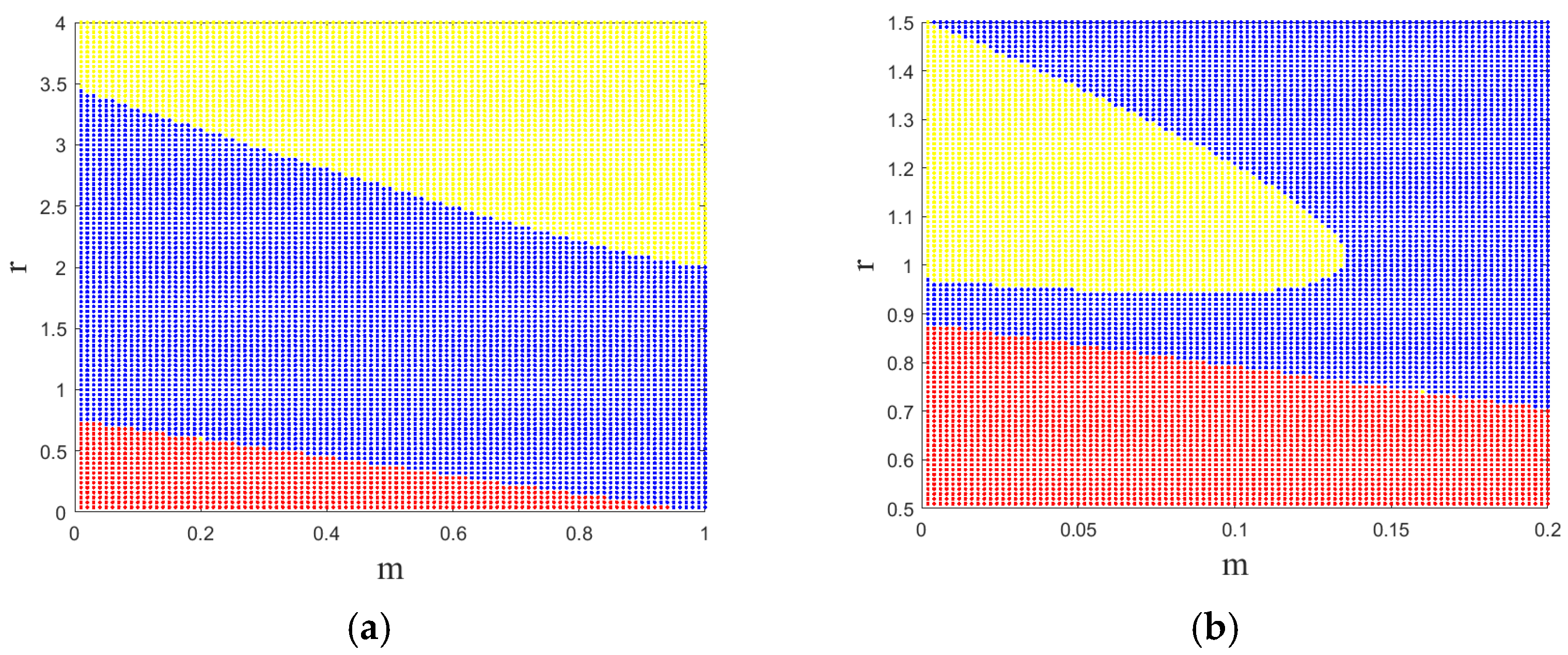
| m | The proportion of prey protected by refuge | 0~1 | 0~0.45 | 0~0.15 | - |
3. Results and Discussion
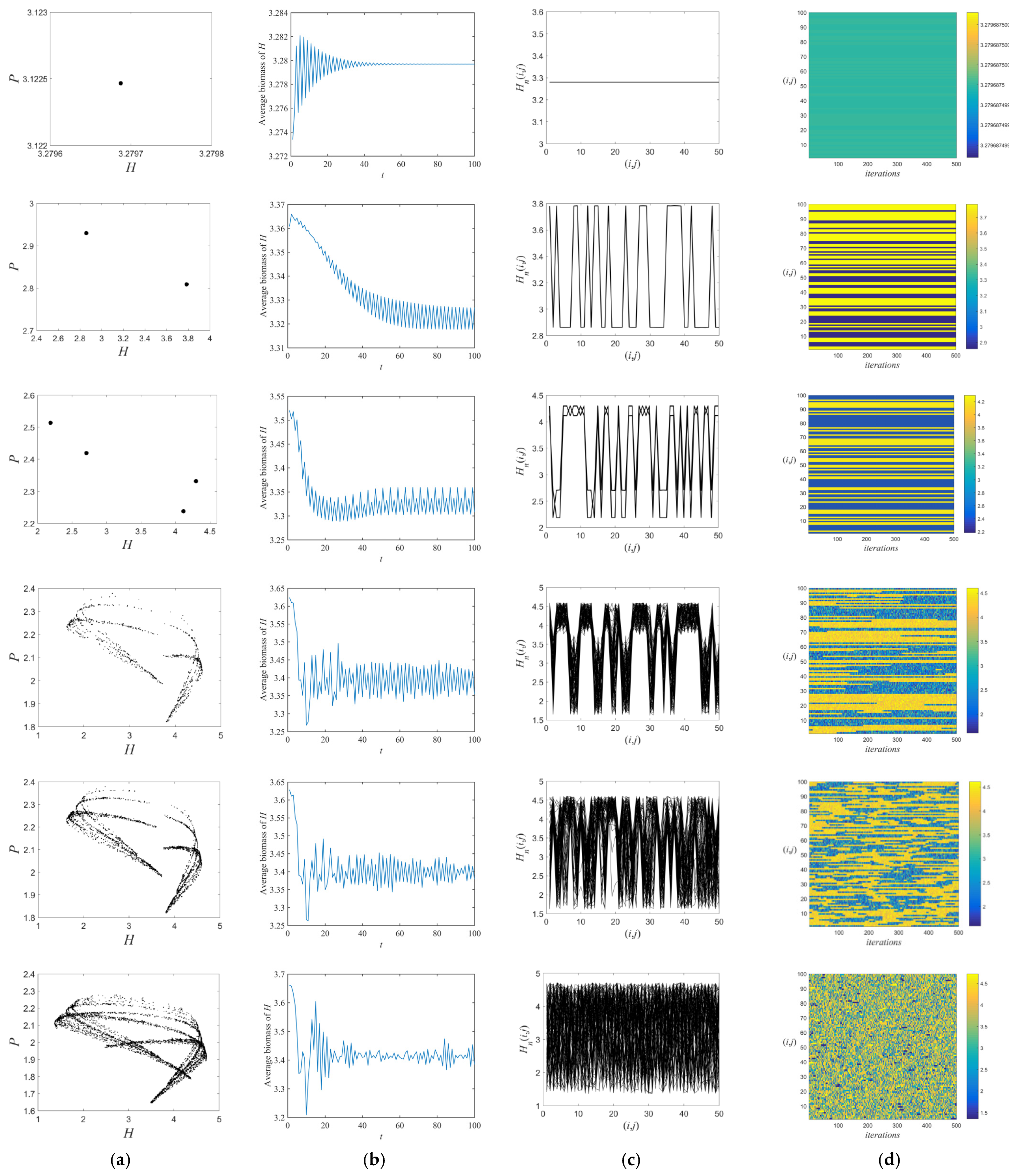
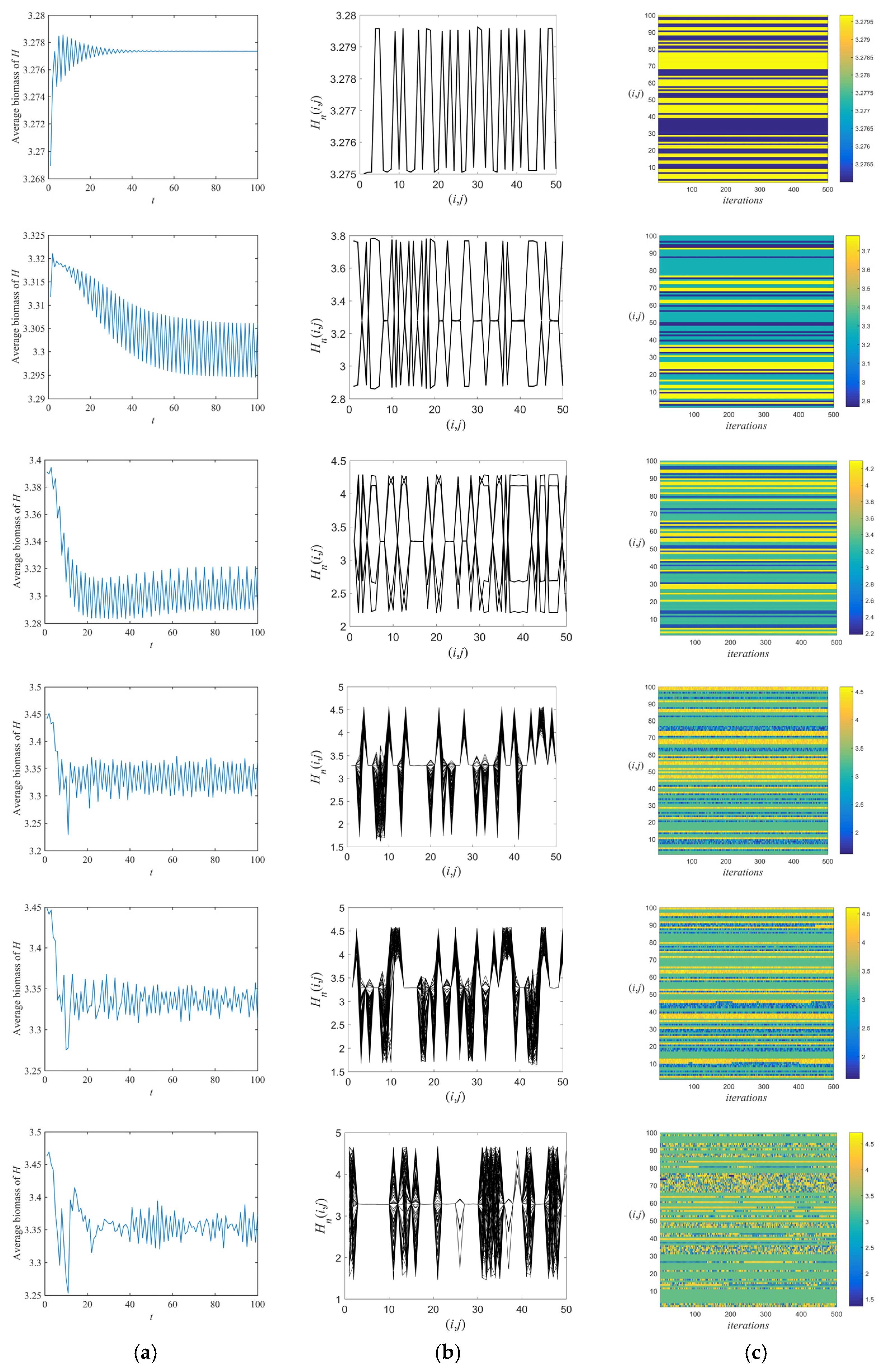
3.1. Flip Bifurcations Produced by Moths with Relatively Higher Growth Rates
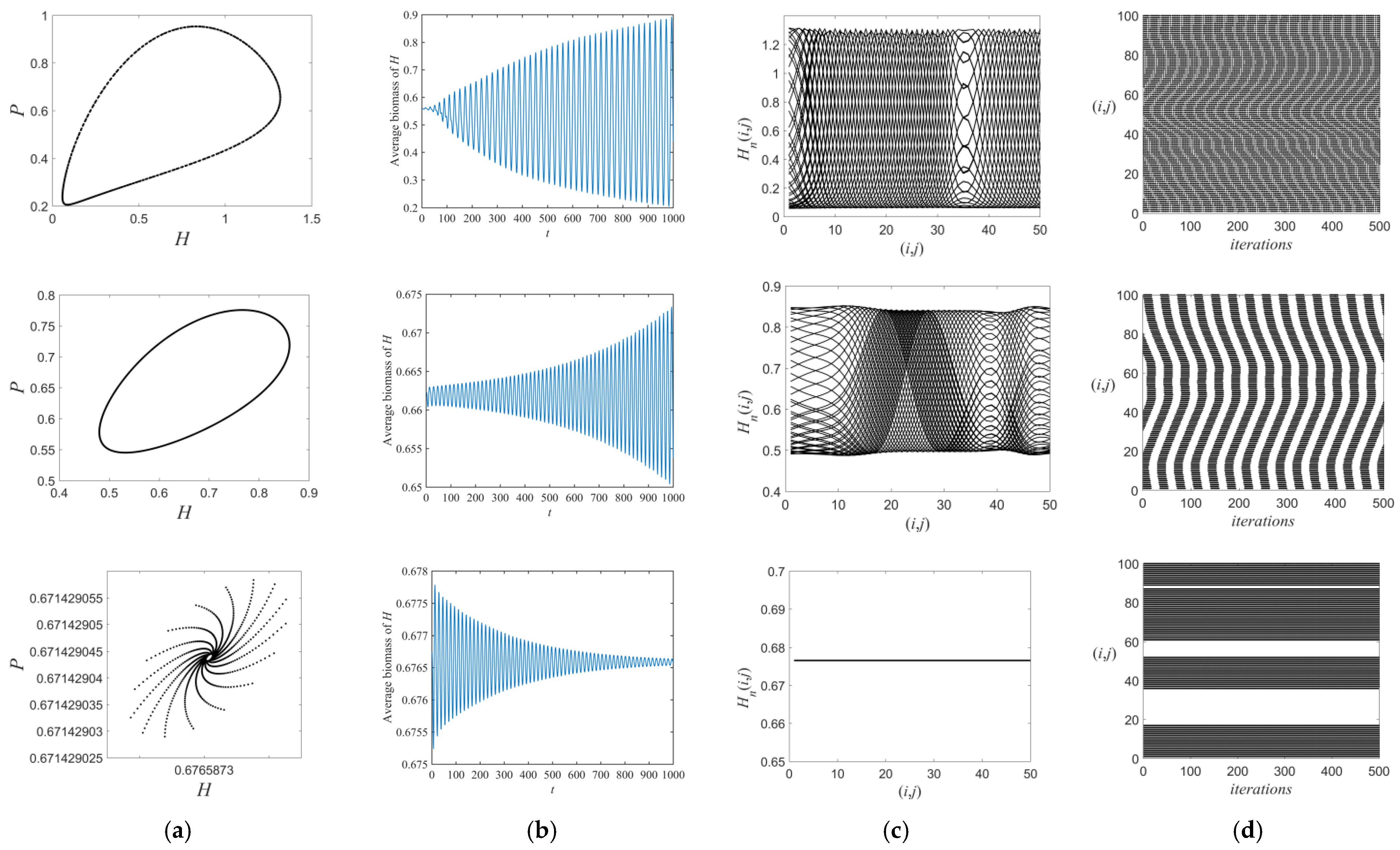
3.2. Neimark–Sacker Bifurcation Produced by Moths with Relatively Lower Growth Rates
4. Conclusions
Author Contributions
Funding
Institutional Review Board Statement
Data Availability Statement
Conflicts of Interest
References
- Khaliq, A.; Javed, M.; Sohail, M.; Sagheer, M. Environmental Effects on Insects and Their Population Dynamics. J. Entomol. Zool. Stud. 2014, 2, 1–7. [Google Scholar]
- Logan, J.A.; Allen, J.C. Nonlinear Dynamics and Chaos in Insect Populations. Annu. Rev. Entomol. 1992, 37, 455–477. [Google Scholar] [CrossRef]
- Badran, F.; Fathipour, Y.; Bagheri, A.; Attaran, M.; Reddy, G.V.P. Generation-Dependent Functional and Numerical Responses of a Naturally Fungus-Infected Colony of Habrobracon hebetor (Hymenoptera: Braconidae) Reared on Ephestia kuehniella (Lepidoptera: Pyralidae) in Iran. J. Econ. Entomol. 2021, 114, 62–71. [Google Scholar] [CrossRef] [PubMed]
- Nath, R.K.; Saikia, D.K.; Kalita, S. Life Table and Budgeting of Plassey Borer, Chilo Tumidicostalis hampson (Lepidoptera: Pyralidae). Int. J. Trop. Insect Sci. 2022, 42, 2073–2082. [Google Scholar] [CrossRef]
- Weaving, H.; Terblanche, J.S.; Pottier, P.; English, S. Meta-Analysis Reveals Weak but Pervasive Plasticity in Insect Thermal Limits. Nat. Commun. 2022, 13, 5292. [Google Scholar] [CrossRef]
- Polášková, V.; Bojková, J.; Polášek, M.; Šorfová, V.; Horsák, M. Water Temperature Stability Modulates Insect Thermal Responses at Spring Fens. Hydrobiologia 2022, 849, 4693–4706. [Google Scholar] [CrossRef]
- Zhao, L.; Gao, R.; Liu, J.; Liu, L.; Li, R.; Men, L.; Zhang, Z. Effects of Environmental Factors on the Spatial Distribution Pattern and Diversity of Insect Communities along Altitude Gradients in Guandi Mountain, China. Insects 2023, 14, 224. [Google Scholar] [CrossRef]
- Santos-Neto, P.E.; Arnan, X.; Ribeiro-Neto, J.D.; Wirth, R.; Leal, I.R. Aridity, but Not Disturbance, Reduces the Specialization and Modularity of Plant–Insect Herbivore Interaction Networks in Caatinga Dry Forest. J. Insect Conserv. 2022, 26, 175–189. [Google Scholar] [CrossRef]
- Jiang, B.; Yao, Y.; Mauersberger, R.; Mikolajewski, D.J. Allometry of Defense: Predator Shift Alters Ontogenetic Growth Patterns in an Antipredator Trait. Insects 2023, 14, 712. [Google Scholar] [CrossRef]
- Ghosh, S.; Bhattacharyya, S. A Two-Patch Prey-Predator Model with Food-Gathering Activity. J. Appl. Math. Comput. 2011, 37, 497–521. [Google Scholar] [CrossRef]
- Abbate, S.L.; Madeira, F.; Bentancur, O.; Altier, N.; Pons, X. Refuge Areas Favor the Presence of Predators and Herbivores in Bt Soybean: A Landscape Perspective. J. Pest Sci. 2023, 96, 1133–1147. [Google Scholar] [CrossRef]
- Widick, I.V.; Berl, J.L.; Kaplan, I.; Zollner, P.A.; Blubaugh, C.K. The Fear Diet: Risk, Refuge, and Biological Control by Omnivorous Weed Seed Predators. Basic Appl. Ecol. 2022, 65, 50–61. [Google Scholar] [CrossRef]
- Brewer, T.R.; Bonsall, M.B. Combining Refuges with Transgenic Insect Releases for the Management of an Insect Pest with Non-Recessive Resistance to Bt Crops in Agricultural Landscapes. J. Theor. Biol. 2021, 509, 110514. [Google Scholar] [CrossRef] [PubMed]
- Menezes, L.C.C.R.; Rossi, M.N.; Godoy, W.A.C. The Effect of Refuge on Dermestes ater (Coleoptera: Dermestidae) Predation on Musca domestica (Diptera: Muscidae): Refuge for Prey or the Predator? J. Insect Behav. 2006, 19, 717–729. [Google Scholar] [CrossRef]
- Human, D.J.; Potgieter, L. Landscape Configurations of Refuge Areas That Delay the Evolution of Resistance to Bt Sugarcane: An Agent Based Modeling Approach. J. Econ. Entomol. 2023, 116, 1360–1371. [Google Scholar] [CrossRef]
- De Grandpré, L.; Marchand, M.; Kneeshaw, D.D.; Paré, D.; Boucher, D.; Bourassa, S.; Gervais, D.; Simard, M.; Griffin, J.M.; Pureswaran, D.S. Defoliation-Induced Changes in Foliage Quality May Trigger Broad-Scale Insect Outbreaks. Commun. Biol. 2022, 5, 463. [Google Scholar] [CrossRef]
- May, R.M. Will a Large Complex System Be Stable? Nature 1972, 238, 413–414. [Google Scholar] [CrossRef]
- Rogers, T.L.; Johnson, B.J.; Munch, S.B. Chaos Is Not Rare in Natural Ecosystems. Nat. Ecol. Evol. 2022, 6, 1105–1111. [Google Scholar] [CrossRef]
- Yuan, S.; Li, Y.; Zeng, Z. Stochastic Bifurcations and Tipping Phenomena of Insect Outbreak Systems Driven by α-Stable Lévy Processes. Math. Model. Nat. Phenom. 2022, 17, 34. [Google Scholar] [CrossRef]
- Haynes, K.J.; Walter, J.A. Advances in Understanding the Drivers of Population Spatial Synchrony. Curr. Opin. Insect Sci. 2022, 53, 100959. [Google Scholar] [CrossRef]
- Lantschner, M.V.; Aukema, B.H.; Corley, J.C. Droughts Drive Outbreak Dynamics of an Invasive Forest Insect on an Exotic Host. For. Ecol. Manag. 2019, 433, 762–770. [Google Scholar] [CrossRef]
- Macarthur, R.H. Patterns of Species Diversity. Biol. Rev. 1965, 40, 510–533. [Google Scholar] [CrossRef]
- MacArthur, R.H.; Wilson, E.O. An Equilibrium Theory of Insular Zoogeography. Evolution 1963, 17, 373. [Google Scholar] [CrossRef]
- Senior, L.J.; Healey, M.A.; Wright, C.L. The Role of Spiders as Predators of Two Lepidopteran Brassica Pests: Spiders as Predators of Brassica Pests. Austral Entomol. 2016, 55, 383–391. [Google Scholar] [CrossRef]
- Huang, X.; Quan, X.; Wang, X.; Yun, Y.; Peng, Y. Is the Spider a Good Biological Control Agent for Plutella xylostella (Lepidoptera: Plutellidae)? Zoologia 2018, 35, e23481. [Google Scholar] [CrossRef]
- Mishra, A.; Kumar, B.; Rastogi, N. Do the Food Availability Conditions Influence the Stage-Specific Prey Choice and Predation Attributes of Agroecosystem-Inhabiting Spiders? Trop. Ecol. 2022, 63, 433–439. [Google Scholar] [CrossRef]
- Xiang, C.; Huang, J.; Wang, H. Bifurcations in Holling-Tanner Model with Generalist Predator and Prey Refuge. J. Differ. Equ. 2023, 343, 495–529. [Google Scholar] [CrossRef]
- Agiza, H.N.; ELabbasy, E.M.; EL-Metwally, H.; Elsadany, A.A. Chaotic Dynamics of a Discrete Prey–Predator Model with Holling Type II. Nonlinear Anal. Real World Appl. 2009, 10, 116–129. [Google Scholar] [CrossRef]
- Singh, A.; Sharma, V.S. Bifurcations and Chaos Control in a Discrete-Time Prey–Predator Model with Holling Type-II Functional Response and Prey Refuge. J. Comput. Appl. Math. 2023, 418, 114666. [Google Scholar] [CrossRef]
- Zhang, C.; Li, X. Dynamics of a Discrete Leslie–Gower Model with Harvesting and Holling-II Functional Response. Mathematics 2023, 11, 3303. [Google Scholar] [CrossRef]
- Balcı, E. Predation Fear and Its Carry-over Effect in a Fractional Order Prey–Predator Model with Prey Refuge. Chaos Solitons Fractals 2023, 175, 114016. [Google Scholar] [CrossRef]
- Rao, F.; Kang, Y. Dynamics of a Stochastic Prey–Predator System with Prey Refuge, Predation Fear and Its Carry-Over Effects. Chaos Solitons Fractals 2023, 175, 113935. [Google Scholar] [CrossRef]
- Wang, S.; Tang, H.; Ma, Z. Hopf Bifurcation of a Multiple-Delayed Predator–Prey System with Habitat Complexity. Math. Comput. Simul. 2021, 180, 1–23. [Google Scholar] [CrossRef]
- Ma, Z.; Chen, F.; Wu, C.; Chen, W. Dynamic Behaviors of a Lotka–Volterra Predator–Prey Model Incorporating a Prey Refuge and Predator Mutual Interference. Appl. Math. Comput. 2013, 219, 7945–7953. [Google Scholar] [CrossRef]
- Khajanchi, S.; Banerjee, S. Role of Constant Prey Refuge on Stage Structure Predator–Prey Model with Ratio Dependent Functional Response. Appl. Math. Comput. 2017, 314, 193–198. [Google Scholar] [CrossRef]
- Chen, L.; Chen, F.; Chen, L. Qualitative Analysis of a Predator–Prey Model with Holling Type II Functional Response Incorporating a Constant Prey Refuge. Nonlinear Anal. Real World Appl. 2010, 11, 246–252. [Google Scholar] [CrossRef]
- Guan, X.; Wang, W.; Cai, Y. Spatiotemporal Dynamics of a Leslie–Gower Predator–Prey Model Incorporating a Prey Refuge. Nonlinear Anal. Real World Appl. 2011, 12, 2385–2395. [Google Scholar] [CrossRef]
- Elaydi, S.N. Discrete Chaos: With Applications in Science and Engineering, 2nd ed.; CRC Press: Philadelphia, PA, USA, 2007; ISBN 978-0-429-14919-1. [Google Scholar]
- Elaydi, S.; Luís, R. Open Problems in Some Competition Models. J. Differ. Equ. Appl. 2011, 17, 1873–1877. [Google Scholar] [CrossRef]
- Nayfeh, A.; Balachandran, B. Applied Nonlinear Dynamics: Analytical, Computational, and Experimental Methods. Wiley Intersci. 1995, 32, 32. [Google Scholar] [CrossRef]
- Guzowska, M.; Luís, R.; Elaydi, S. Bifurcation and Invariant Manifolds of the Logistic Competition Model. J. Differ. Equ. Appl. 2011, 17, 1851–1872. [Google Scholar] [CrossRef]
- Luís, R.; Elaydi, S.; Oliveira, H. Stability of a Ricker-Type Competition Model and the Competitive Exclusion Principle. J. Biol. Dyn. 2011, 5, 636–660. [Google Scholar] [CrossRef]
- Suhubi, E.S. Nonlinear Oscillations, Dynamical Systems, and Bifurcations of Vector Fields. Int. J. Eng. Sci. 1988, 26, 221–222. [Google Scholar] [CrossRef]
- Wen, G. Criterion to Identify Hopf Bifurcations in Maps of Arbitrary Dimension. Phys. Rev. E 2005, 72, 026201. [Google Scholar] [CrossRef]
- Zhang, Y.-Q.; He, Y.; Wang, X.-Y. Spatiotemporal Chaos in Mixed Linear–Nonlinear Two-Dimensional Coupled Logistic Map Lattice. Phys. A Stat. Mech. Its Appl. 2018, 490, 148–160. [Google Scholar] [CrossRef]
- Gkana, A.; Zachilas, L. Incorporating Prey Refuge in a Prey–Predator Model with a Holling Type I Functional Response: Random Dynamics and Population Outbreaks. J. Biol. Phys. 2013, 39, 587–606. [Google Scholar] [CrossRef]
- Han, W.; Zhang, S.; Shen, F.; Liu, M.; Ren, C.; Gao, X. Residual Toxicity and Sublethal Effects of Chlorantraniliprole on Plutella xylostella (Lepidoptera: Plutellidae): Toxicity of Chlorantraniliprole to P. xylostella. Pest Manag. Sci. 2012, 68, 1184–1190. [Google Scholar] [CrossRef] [PubMed]
- Haripriya, K.; Kennedy, J.S.; Geethalakshmi, V.; Rajabaskar, D. Effect of Elevated Carbon Dioxide on the Fitness Traits of Plutella xylostella (L.) (Lepidoptera: Plutellidae). Int. J. Pest Manag. 2024, 70, 14–22. [Google Scholar] [CrossRef]
- Ludwig, D.; Jones, D.D.; Holling, C.S. Qualitative Analysis of Insect Outbreak Systems: The Spruce Budworm and Forest. J. Anim. Ecol. 1978, 47, 315. [Google Scholar] [CrossRef]
- Mishra, A.; Kumar, B.; Rastogi, N. Predation Potential of Hunting and Web-Building Spiders on Rice Pests of Indian Subcontinent. Int. J. Trop. Insect Sci. 2021, 41, 1027–1036. [Google Scholar] [CrossRef]
- Kar, T.K. Stability Analysis of a Prey–Predator Model Incorporating a Prey Refuge. Commun. Nonlinear Sci. Numer. Simul. 2005, 10, 681–691. [Google Scholar] [CrossRef]
- Zhou, Y.; Sun, W.; Song, Y.; Zheng, Z.; Lu, J.; Chen, S. Hopf Bifurcation Analysis of a Predator–Prey Model with Holling-II Type Functional Response and a Prey Refuge. Nonlinear Dyn. 2019, 97, 1439–1450. [Google Scholar] [CrossRef]
- Liman, A.; Eklund, K.; Björkman, C. Predator Refuges for Conservation Biological Control in an Intermediately Disturbed System: The Rise and Fall of a Simple Solution. J. Appl. Ecol. 2016, 53, 1823–1830. [Google Scholar] [CrossRef]
- Banko, P.C.; Peck, R.W.; Yelenik, S.G.; Paxton, E.H.; Bonaccorso, F.; Montoya-Aiona, K.; Hughes, R.F.; Perakis, S. Hypotheses and Lessons from a Native Moth Outbreak in a Low-diversity, Tropical Rainforest. Ecosphere 2022, 13, e3926. [Google Scholar] [CrossRef]
- Ma, Z.; Li, W.; Zhao, Y.; Wang, W.; Zhang, H.; Li, Z. Effects of Prey Refuges on a Predator–Prey Model with a Class of Functional Responses: The Role of Refuges. Math. Biosci. 2009, 218, 73–79. [Google Scholar] [CrossRef] [PubMed]
- Zhang, Y.-Q.; Wang, X.-Y. Spatiotemporal Chaos in Mixed Linear–Nonlinear Coupled Logistic Map Lattice. Phys. A Stat. Mech. Its Appl. 2014, 402, 104–118. [Google Scholar] [CrossRef]


Disclaimer/Publisher’s Note: The statements, opinions and data contained in all publications are solely those of the individual author(s) and contributor(s) and not of MDPI and/or the editor(s). MDPI and/or the editor(s) disclaim responsibility for any injury to people or property resulting from any ideas, methods, instructions or products referred to in the content. |
© 2024 by the authors. Licensee MDPI, Basel, Switzerland. This article is an open access article distributed under the terms and conditions of the Creative Commons Attribution (CC BY) license (https://creativecommons.org/licenses/by/4.0/).
Share and Cite
Zhang, H.; Yuan, X.; Zou, H.; Zhao, L.; Wang, Z.; Guo, F.; Liu, Z. The Spatiotemporal Dynamics of Insect Predator–Prey System Incorporating Refuge Effect. Entropy 2024, 26, 196. https://doi.org/10.3390/e26030196
Zhang H, Yuan X, Zou H, Zhao L, Wang Z, Guo F, Liu Z. The Spatiotemporal Dynamics of Insect Predator–Prey System Incorporating Refuge Effect. Entropy. 2024; 26(3):196. https://doi.org/10.3390/e26030196
Chicago/Turabian StyleZhang, Huayong, Xiaotong Yuan, Hengchao Zou, Lei Zhao, Zhongyu Wang, Fenglu Guo, and Zhao Liu. 2024. "The Spatiotemporal Dynamics of Insect Predator–Prey System Incorporating Refuge Effect" Entropy 26, no. 3: 196. https://doi.org/10.3390/e26030196
APA StyleZhang, H., Yuan, X., Zou, H., Zhao, L., Wang, Z., Guo, F., & Liu, Z. (2024). The Spatiotemporal Dynamics of Insect Predator–Prey System Incorporating Refuge Effect. Entropy, 26(3), 196. https://doi.org/10.3390/e26030196