Abstract
We study Einstein’s gravity coupled to nonlinear electrodynamics with two parameters in anti-de Sitter spacetime. Magnetically charged black holes in an extended phase space are investigated. We obtain the mass and metric functions and the asymptotic and corrections to the Reissner–Nordström metric function when the cosmological constant vanishes. The first law of black hole thermodynamics in an extended phase space is formulated and the magnetic potential and the thermodynamic conjugate to the coupling are obtained. We prove the generalized Smarr relation. The heat capacity and the Gibbs free energy are computed and the phase transitions are studied. It is shown that the electric fields of charged objects at the origin and the electrostatic self-energy are finite within the nonlinear electrodynamics proposed.
1. Introduction
It is understood that the black hole area plays the role of entropy and the temperature is connected with the surface gravity [1,2,3,4,5]. The importance of gravity in AdS spacetime is due to the holographic principle (a gauge duality description) [6], which has applications in condensed matter physics. Firstly, black hole phase transitions in Schwarzschild–AdS spacetime were studied in Ref. [7]. The negative cosmological constant, in an extended-phase-space black hole thermodynamics, is linked with the thermodynamic pressure conjugated to the volume [8,9,10,11]. The cosmological constant variation was included in the first law of black hole thermodynamics in Refs. [12,13,14,15,16,17]. However, within general relativity, the cosmological constant is a fixed external parameter. Moreover, such variation in in the first law of black hole thermodynamics means the consideration of black hole ensembles possessing different asymptotics. This point of view is different from that of standard black hole thermodynamics, where the parameters are varied but the AdS background is fixed. There are some reasons to consider the variation in in black hole thermodynamics. First of all, physical constants can arise as the vacuum expectation values are not fixed a priori and therefore may vary. As a result, these ‘constants’ are not real constants and may be included in the first law of black hole thermodynamics [18,19]. The second reason is that, without varying the cosmological constant, the Smarr relation is inconsistent with the first law of black hole thermodynamics [13]. When is inserted in the first law of black hole thermodynamics, the mass M of the black hole should be treated as enthalpy but not internal energy [13]. The first law of black hole thermodynamics can be formulated within Einstein’s gravity if one includes the term. This requires us to introduce a negative cosmological constant as a positive pressure . As a result, we come to AdS spacetime. It should be noted that the thermodynamic pressure P is different from the local pressure that is present in the energy–momentum tensor. The conjugate variable to P is the thermodynamic volume , where is the event horizon radius of a black hole.
In this paper, we study Einstein–AdS gravity coupled to nonlinear electrodynamics (NED) with two parameters, proposed here, that allow us to smooth out singularities. The first NED was Born–Infeld electrodynamics [20]; without the singularities of point-like particles possessing finite electric self-energy at the weak-field limit, it is converted into Maxwell’s theory. Our NED model has similar behavior. We study magnetic black holes and their thermodynamics in Einstein–AdS gravity in the extended phase space. The NED model, with coupling and dimensionless parameter , proposed here, is of interest because it includes model [21] for . This unified approach allows us to find similarities and differences for different models.
The structure of the paper is as follows. In Section 2, we find the mass and metric functions and their asymptotics. Corrections to the Reissner–Nordström metric function are obtained when the cosmological constant is zero. We prove the first law of black hole thermodynamics in an extended phase space and obtain the magnetic potential and the thermodynamic conjugate to the coupling. The generalized Smarr formula is proven. The Gibbs free energy is calculated and depicted for some parameters and the phase transitions are studied in Section 3. In Appendix A, we obtain the electric fields of charged objects and corrections to Coulomb’s law. We show that the electrostatic self-energy of charged particles is finite in Appendix B. In Appendix C, we obtain the metric that is a solution to the Einstein–Maxwell system. Section 4 is a discussion of the results obtained.
We use units with .
2. Einstein–AdS Black Hole Solution
The action of Einstein’s gravity in AdS spacetime is given by
where G is the gravitational constant, is the negative cosmological constant, and l is the AdS radius. We propose the NED Lagrangian as follows:
where is the Lorenz invariant and E and B are the electric and magnetic fields, correspondingly. The coupling has the dimension , and the dimensionless parameter . The weak-field limit of Lagrangian (2) is Maxwell’s Lagrangian. Lagrangian (2) at becomes the rational NED Lagrangian [22]. The NED Lagrangian (2) for some values of was used in the inflation scenario [23,24,25]. From action (1), one finds the Einstein and field equations
where . The energy–stress tensor reads
We consider here spherical symmetry with the line element
Magnetic black holes possess the magnetic field , where q is the magnetic charge. The metric function is given by (see Appendix C and [26])
with the mass function
where is an integration constant (the Schwarzschild mass) and is the energy density. We obtain the energy density
where the magnetic energy density found from Equations (2) and (5) is
Making use of Equations (8) and (9), we obtain the mass function
where is the hypergeometric function. The magnetic energy is given by
where is the Gamma function. Equation (11) shows that, at Maxwell’s limit , the black hole’s magnetic mass diverges. Therefore, a smooth limit to Maxwell’s theory is questionable. From Equations (7) and (10), one finds the metric function
We employ the relation [27]
for , which will be used to obtain the asymptotic of the metric function as . When the Schwarzschild mass is zero () and as , the asymptotic is
Equation (14) shows that, at , a singularity of the metric function is absent. In addition, to avoid a conical singularity at , we also should set (). It is worth noting that the magnetic energy density is finite at only if . Therefore, to have regular black holes, one has to assume that . Then, from Equation (14), we find , which is a necessary condition to have regular spacetime. We explore the transformation [27]
to obtain the asymptotic of the metric function as . By virtue of Equations (13) and (15), we find
where the relations and are used. Making use of Equations (13) and (16) as when the cosmological constant vanishes (), we find
where is the ADM mass (the total black hole mass as ). It follows from Equation (17) that the corrections to the Reissner–Nordström solution are in the order of . When , metric function (17) is converted into the Reissner–Nordström metric function. The plot of metric function (12) is given in Figure 1 with , , , .
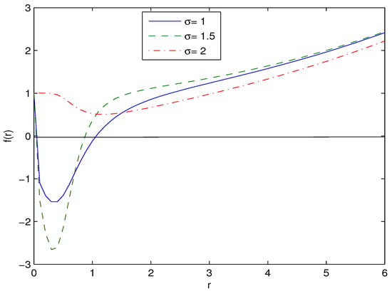
Figure 1.
The function at , , , , . Figure 1 shows that black holes may have one or two horizons. When increases, the event horizon radius decreases.
In accordance with Figure 1, if parameter increases, the event horizon radius decreases. Figure 1 shows that black holes can have one or two horizons. It should be noted that when we set as in Figure 1, we come to Planckian units [28]. Then, in this case, if one has, for example, dimensionless event horizon radius (as in Figure 1), in the usual units, cm, where is Planck’s length. When the dimensionless mass is , for example, in the usual units, g, where is Planck’s mass. Because, in Figure 1 the event horizon radius is small, we have here the example of tiny black holes (primordial black holes). Such black holes could have been created after the Big Bang. It is worth noting that such an example of quantum-sized black holes is described here by semiclassical gravity.
3. First Law of Black Hole Thermodynamics
The pressure, in extended-phase-space thermodynamics, is defined as [13,14,17,29]. The coupling is treated as the thermodynamic value and the mass M is a chemical enthalpy so that and U is the internal energy. In the following, we will use Planckian units with . By using Euler’s dimensional analysis [13,30], we have dimensions , , , , , and
where J is the black hole’s angular momentum. In the following, we consider non-rotating black holes and, therefore, . The thermodynamic conjugate to coupling is (so-called vacuum polarization) [10]. The black hole volume V and entropy S are defined as
From Equation (16) and the equation , where is the event horizon radius, one finds
Making use of Equation (20), we obtain
Here, we have used the relation [27]
Defining the Hawking temperature
where , and by virtue of Equations (16) and (23), we obtain
At in Equation (24), one finds the Maxwell–AdS black hole Hawking temperature. The first law of black hole thermodynamics follows from Equations (19), (20) and (24),
From Equations (21) and (25), we obtain the magnetic potential and the thermodynamic conjugate to coupling (vacuum polarization)
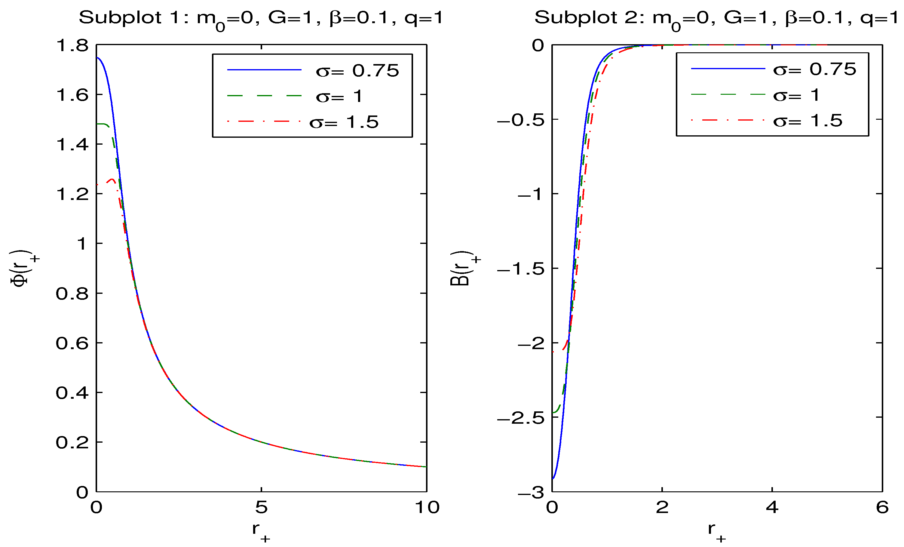
The plots of and versus are depicted in Figure 2.
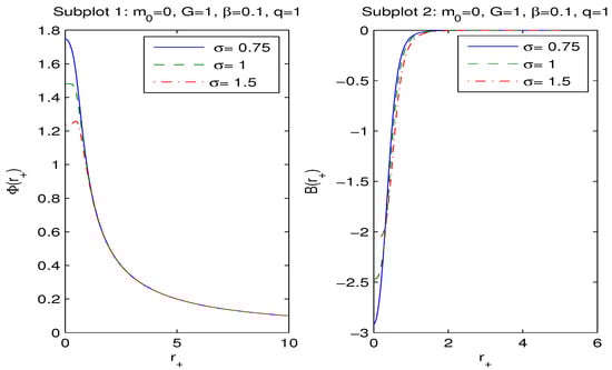
Figure 2.
The functions and vs. at , . The solid curve in subplot 1 is for , the dashed curve is for , and the dashed-dotted curve is for . It follows that the magnetic potential is finite at and becomes zero as . The function , in subplot 2, vanishes as and is finite at .
Figure 2, in the left panel, shows that as , the magnetic potential vanishes (), and at , it is finite. If the parameter increases, decreases. According to the right panel of Figure 2, at , the vacuum polarization is finite, and as , vanishes (). When the parameter increases, also increases. With the aid of Equations (19), (24) and (26), we find the generalized Smarr relation
4. Thermodynamics of Black Holes
To study the local stability of black holes, one can analyze the heat capacity
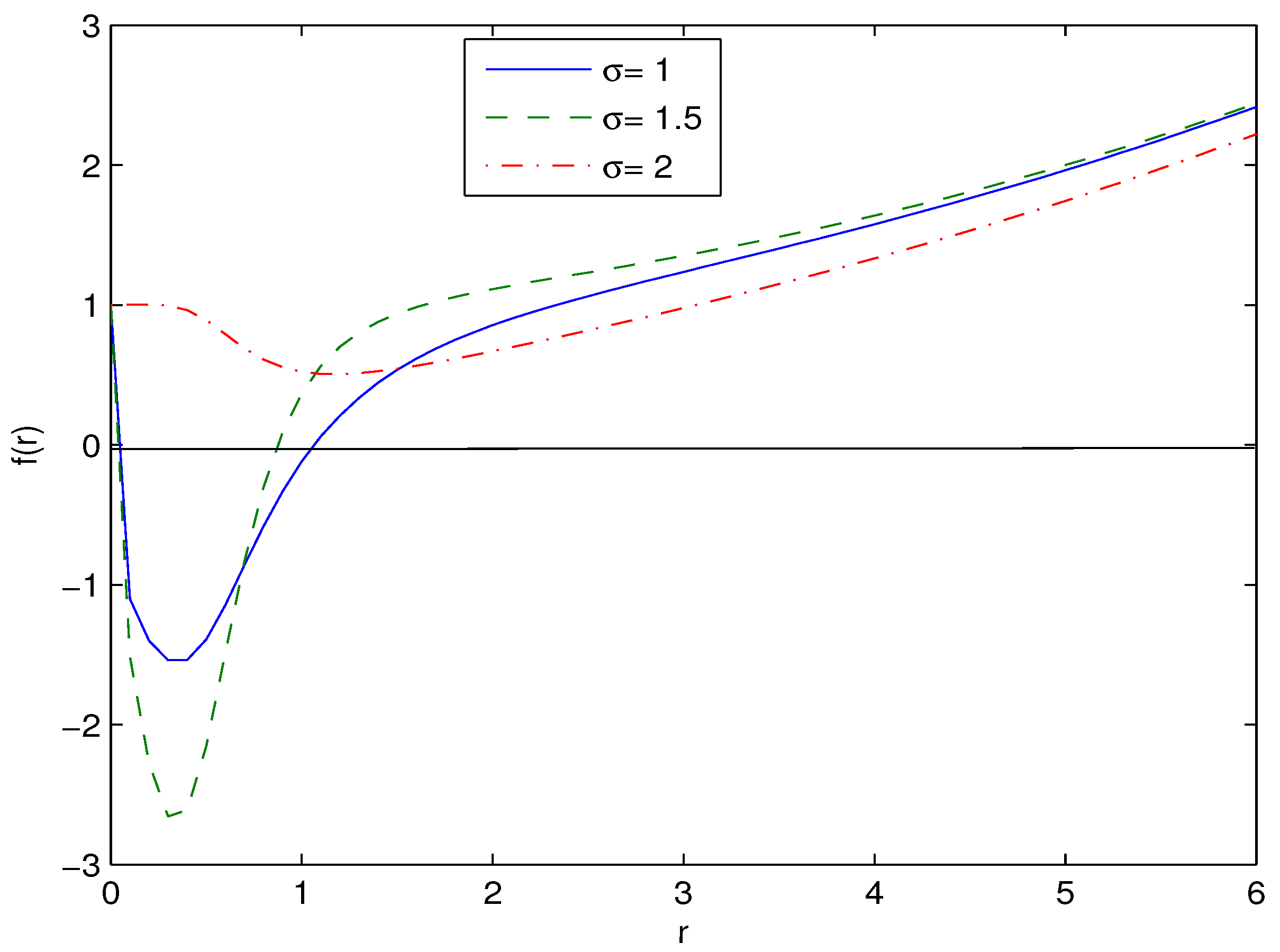
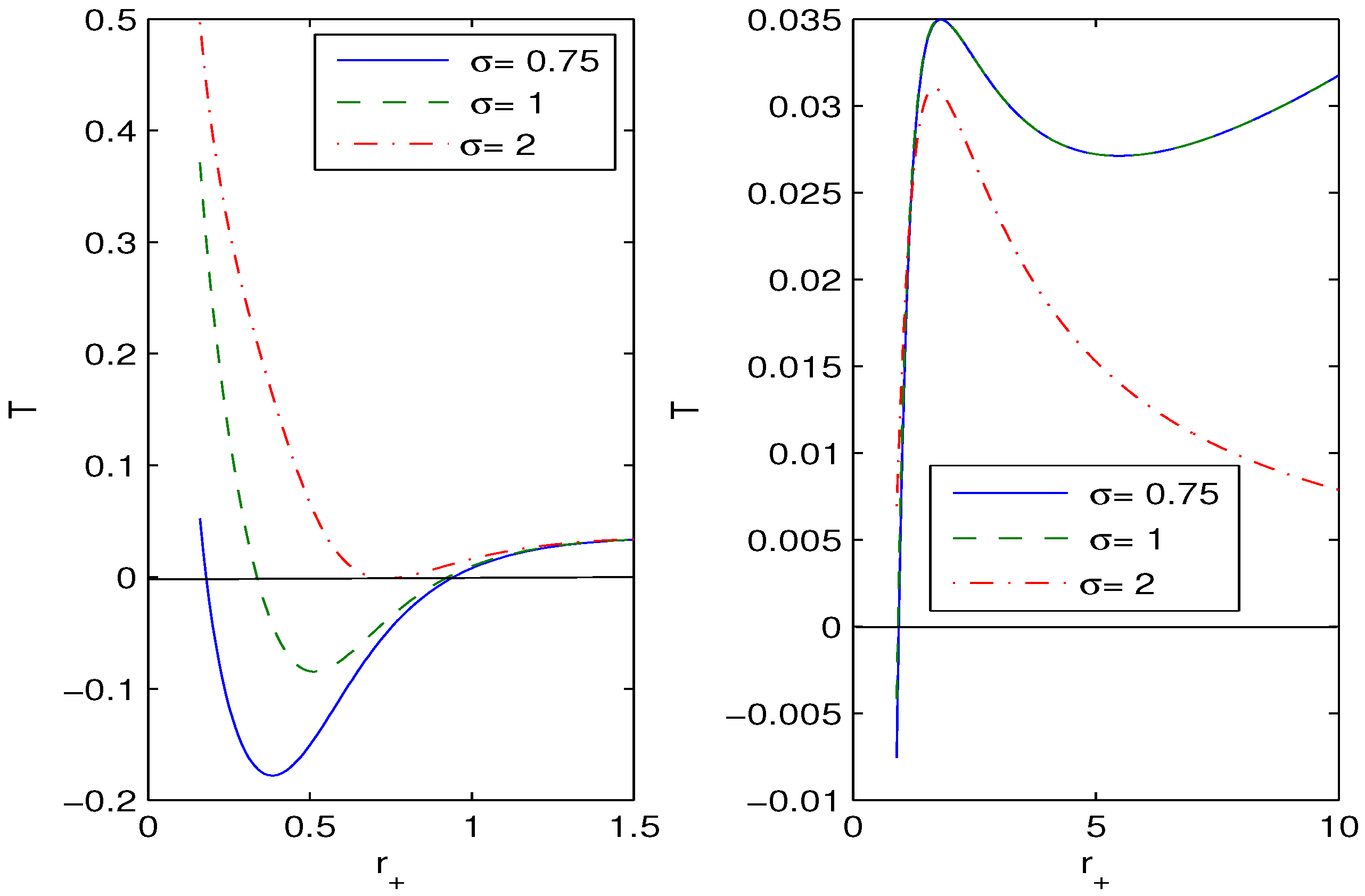
Equation (28) shows that when the Hawking temperature has an extremum, the heat capacity possesses a singularity and the black hole phase transition occurs. With the help of Equation (24), we depict in Figure 3 the Hawking temperature as a function of the event horizon radius.
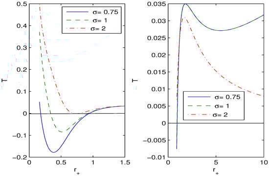
Figure 3.
The functions T vs. at , , . The solid curve in the left panel is for , the dashed curve is for , and the dashed-dotted curve is for . In some intervals of , the Hawking temperature is negative and, therefore, black holes do not exist at these parameters. There are extrema of the Hawking temperature T where the black hole phase transitions occur.
For the case , the analysis of a black hole’s local stability was performed in [21]. The behavior of T and depends on many parameters. By virtue of Equation (24), we obtain
Equations (24) and (29) define the heat capacity (28). Making use of Equations (24), (28) and (29), one can study the heat capacity and the black hole phase transition for different parameters , , q and l.
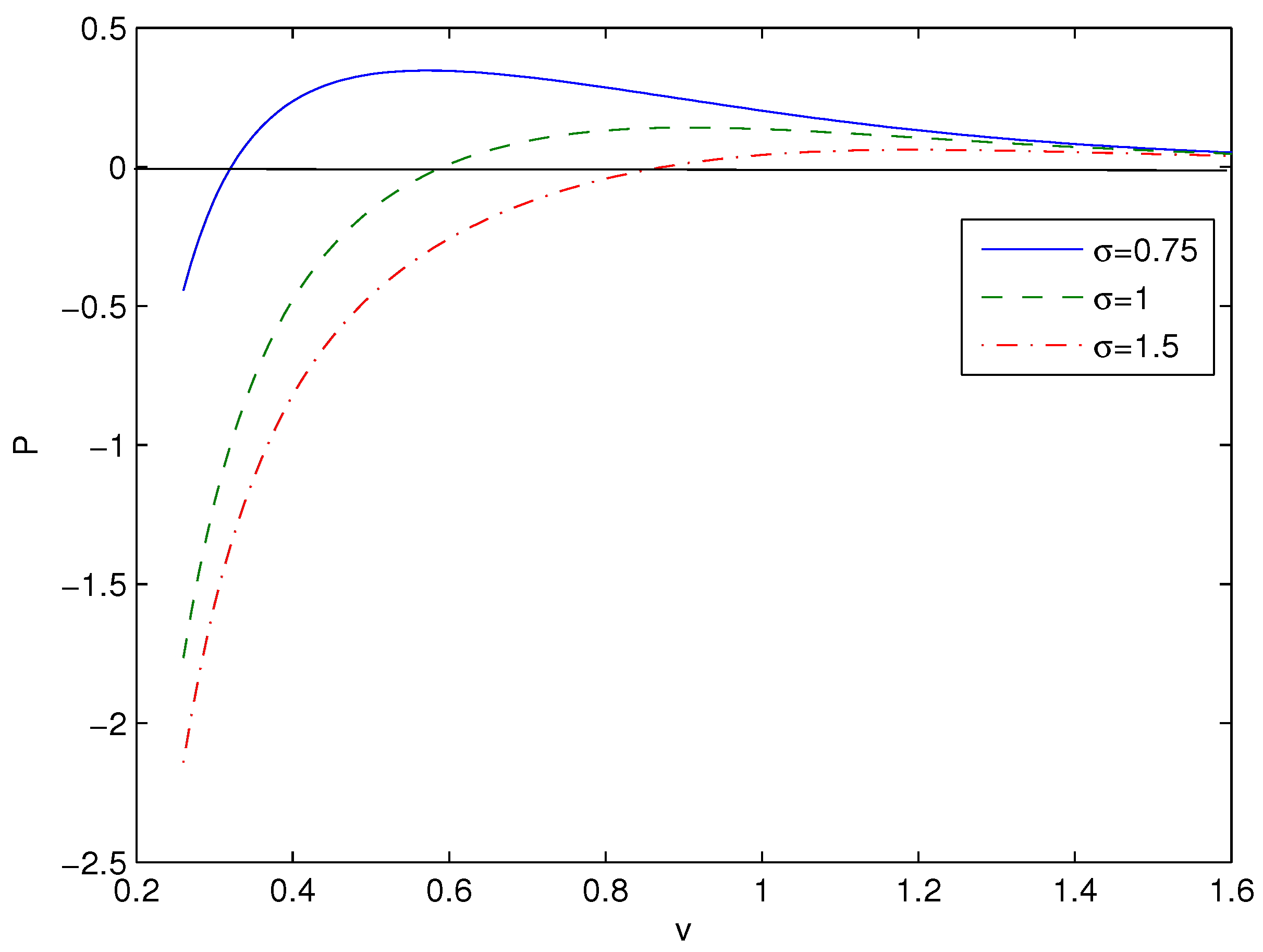
With the help of Equation (24), we obtain the black hole equation of state (EoS):
The specific volume is given by () [11]. Equation (30) is similar to the EoS of the Van der Waals liquid. Placing into expression (30), we obtain
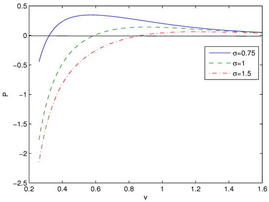
Figure 4.
The functions P vs. v at , , . The solid line is for , the dashed curve is for , and the dashed-dotted curve is for .
The critical points (inflection points) are defined by the equations , , which are complex, so we will not present them here. The analytical solutions for critical points do not exist. The diagrams at the critical values are similar to Van der Waals liquid diagrams having inflection points.
Because M is treated as a chemical enthalpy, the Gibbs free energy reads
Making use of Equations (19), (20), (24) and (32), we obtain
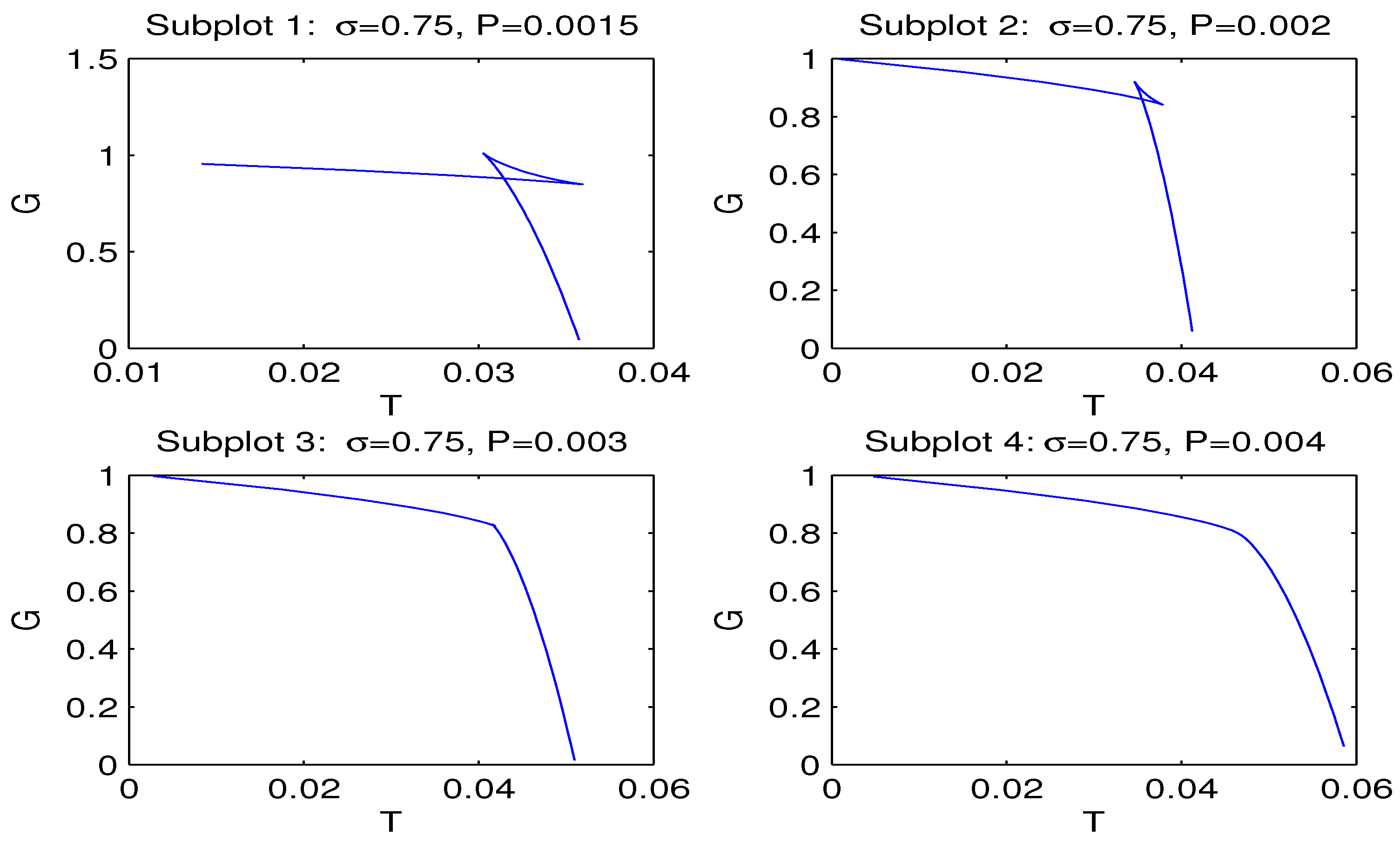
The plot of G versus T is given in Figure 5 for , , .
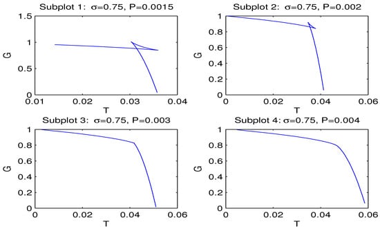
Figure 5.
The functions G vs. T at , , for P = 0.0015, P = 0.002, P = 0.003 and P = 0.004. Subplots 1 and 2 show the critical ’swallowtail’ behavior with first-order phase transitions between small and large black holes. Subplot 3 corresponds to the case of critical points where a second-order phase transition occurs (). Subplot 4 shows the non-critical behavior of the Gibbs free energy.
The critical points and phase transitions of black holes for were studied in [21]. One can investigate black hole phase transitions in our model for an arbitrary with the help of the Gibbs free energy (33). It should be noted that the analytical expressions obtained can be applied for black holes of any sizes. In Figure 1, Figure 2, Figure 3, Figure 4 and Figure 5, we consider examples only for tiny black holes (quantum black holes).
5. Summary
We have obtained magnetic black hole solutions in Einstein–AdS gravity coupled to NED with two parameters, which we propose here. The metric and mass functions and their asymptotics with corrections to the Reissner–Nordström solution, when the cosmological constant is zero, have been found. The total black hole mass includes the Schwarzschild mass and the magnetic mass, which is finite. We have plotted the metric function showing that black holes may have one or two horizons. When parameter increases, the event horizon radius decreases. Figure 2, Figure 3 and Figure 4 show how other physical variables depend on . The black hole thermodynamics in an extended phase space was studied. We formulated the first law of black hole thermodynamics where the pressure is connected with the negative cosmological constant (AdS spacetime) conjugated to the Newtonian geometric volume of the black hole. The thermodynamic potential conjugated to the magnetic charge and the thermodynamic quantity conjugated to coupling (so called vacuum polarization) were computed and plotted. It was proven that the generalized Smarr relation holds for any parameter . We calculated the Hawking temperature, the heat capacity and the Gibbs free energy. Analyses of the first-order and second-order phase transitions were performed for some parameters. The Gibbs free energy showed the critical ‘swallowtail’ behavior, which is similar to the Van der Waals liquid–gas behavior. Figure 5 shows a first-order phase transition with Gibbs free energy that is continuous but not differentiable, but, for a second-order transition, the Gibbs free energy and its first derivatives are continuous. The same feature was first discovered for another model in [11]. It was shown within the NED proposed that the electric fields of charged objects at the origin and the electrostatic self-energy are finite. It should be noted that the first law of electric black hole thermodynamics in Einstein–Born–Infeld theory and other problems were originally studied in Ref. [11].
Funding
This research received no external funding.
Institutional Review Board Statement
Not applicable.
Data Availability Statement
Data sharing is not applicable to this article.
Conflicts of Interest
The authors declare no conflict of interest.
Appendix A
Making use of Equation (4), the Euler–Lagrange equation gives
where
The equation for the electric field, with spherical symmetry and Equation (A1), becomes ()):
By virtue of Equation (A2) and integrating Equation (A3), we obtain
where Q is the electric charge (the integration constant). At , Equation (A4) gives the Coulomb electric field . It is convenient to define unitless variables
Then, Equation (A4) becomes
From Equation (A6), we obtain, for a small x (and small r),
Making use of Equations (A5) and (A7), one finds as
As a result, we have the finite value of the electric field at the origin that is the maximum of the electric field. The plot of y versus x is depicted in Figure A1 for .
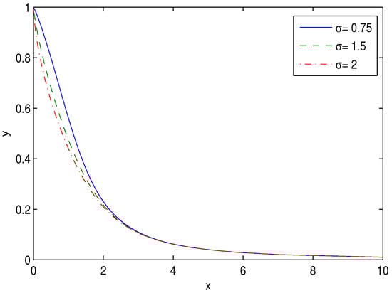
Figure A1.
The function y vs. x at .
Figure A1.
The function y vs. x at .
We obtain, from Equation (A4), as
Equation (A9) shows that the corrections to Coulomb’s law are in the order of . According to Equation (A7) and Figure A1, the electric field is finite at the origin () and becomes zero as . Because of the nonlinearity of electric fields, an electric charge is not a real point-like object and does not possess a singularity at the center.
Appendix B
By virtue of Equation (5), we obtain the electric energy density
Making use of the dimensionless variables (A5), one finds the electric energy density
The total electric energy becomes
where we have used Equation (A6). By numerical calculations of integral (A12), we obtain the dimensionless variables , which are presented in Table A1.

Table A1.
Approximate values of .
Table A1.
Approximate values of .
| 0.1 | 0.2 | 0.3 | 0.4 | 0.5 | 0.6 | 0.7 | 0.8 | 0.9 | 1 | |
|---|---|---|---|---|---|---|---|---|---|---|
| 1.272 | 1.233 | 1.202 | 1.176 | 1.153 | 1.132 | 1.108 | 1.097 | 1.081 | 1.067 |
As a result, in our NED model, the electrostatic energy of charged objects is finite. According to the Abraham and Lorentz idea, the electron mass may be identified with the electromagnetic energy [20,31,32]. Then, one can obtain the parameters and to have the electron mass MeV. Dirac also considered that the electron can be a classical charged object [33].
Appendix C
We will obtain the solution with a magnetic black hole. The component of Einstein’s Equation (3) with spherical symmetry (6) is given by
where
Equation (A13) is a linear first-order equation that belongs to the class of the general equation [34]
with the solution
where C is the integration constant and
Comparing Equations (A13) and (A15), one finds
and , . Then, from Equations (A16)–(A18), we obtain the solution to the component of Einstein’s Equation (A13)
where we use the notations
with .
References
- Bekenstein, J.D. Black holes and entropy. Phys. Rev. D 1973, 7, 2333–2346. [Google Scholar] [CrossRef]
- Hawking, S.W. Particle Creation by Black Holes. Commun. Math. Phys. 1975, 43, 199–220. [Google Scholar] [CrossRef]
- Bardeen, J.M.; Carter, B.; Hawking, S.W. The four laws of black hole mechanics. Commun. Math. Phys. 1973, 31, 161–170. [Google Scholar] [CrossRef]
- Jacobson, T. Thermodynamics of space-time: The Einstein equation of state. Phys. Rev. Lett. 1995, 75, 1260–1263. [Google Scholar] [CrossRef] [PubMed]
- Padmanabhan, T. Thermodynamical Aspects of Gravity: New insights. Rept. Prog. Phys. 2010, 73, 046901. [Google Scholar] [CrossRef]
- Maldacena, J.M. The Large N limit of superconformal field theories and supergravity. Int. J. Theor. Phys. 1999, 38, 1113–1133. [Google Scholar] [CrossRef]
- Hawking, S.W.; Page, D.N. Thermodynamics of Black Holes in anti-de Sitter Space. Commun. Math. Phys. 1983, 87, 577. [Google Scholar] [CrossRef]
- Dolan, B.P. Black holes and Boyle’s law? The thermodynamics of the cosmological constant. Mod. Phys. Lett. A 2015, 30, 1540002. [Google Scholar] [CrossRef]
- Kubiznak, D.; Mann, R.B. Black hole chemistry. Can. J. Phys. 2015, 93, 999–1002. [Google Scholar] [CrossRef]
- Kubiznak, D.; Mann, R.B.; Teo, M. Black hole chemistry: Thermodynamics with Lambda. Class. Quant. Grav. 2017, 34, 063001. [Google Scholar] [CrossRef]
- Gunasekaran, S.; Mann, R.B.; Kubiznak, D. Extended phase space thermodynamics for charged and rotating black holes and Born—Infeld vacuum polarization. J. High Energy Phys. 2012, 1211, 110. [Google Scholar] [CrossRef]
- Caldarelli, M.M.; Cognola, G.; Klemm, D. Thermodynamics of Kerr-Newman-AdS black holes and conformal field theories. Class. Quant. Grav. 2000, 17, 399–420. [Google Scholar] [CrossRef]
- Kastor, D.; Ray, S.; Traschen, J. Enthalpy and the Mechanics of AdS Black Holes. Class. Quant. Grav. 2009, 26, 195011. [Google Scholar] [CrossRef]
- Dolan, B. The cosmological constant and the black hole equation of state. Class. Quant. Grav. 2011, 28, 125020. [Google Scholar] [CrossRef]
- Dolan, B.P. Pressure and volume in the first law of black hole thermodynamics. Class. Quant. Grav. 2011, 28, 235017. [Google Scholar] [CrossRef]
- Dolan, B.P. Compressibility of rotating black holes. Phys. Rev. D 2011, 84, 127503. [Google Scholar] [CrossRef]
- Cvetic, M.; Gibbons, G.; Kubiznak, D.; Pope, C. Black Hole Enthalpy and an Entropy Inequality for the Thermodynamic Volume. Phys. Rev. D 2011, 84, 024037. [Google Scholar] [CrossRef]
- Gibbons, G.W.; Kallosh, R.; Kol, B. Moduli, scalar charges, and the first law of black hole thermodynamics. Phys. Rev. Lett. 1996, 77, 4992–4995. [Google Scholar] [CrossRef]
- Creighton, J.; Mann, R.B. Quasilocal thermodynamics of dilaton gravity coupled to gauge fields. Phys. Rev. D 1995, 52, 4569–4587. [Google Scholar] [CrossRef]
- Born, M.; Infeld, L. Foundations of the new field theory. Proc. Royal Soc. 1934, 144, 425–451. [Google Scholar] [CrossRef]
- Kruglov, S.I. Rational non-linear electrodynamics of AdS black holes and extended phase space thermodynamics. Eur. Phys. J. C 2022, 82, 292. [Google Scholar] [CrossRef]
- Kruglov, S.I. A model of nonlinear electrodynamics. Ann. Phys. 2014, 353, 299–306. [Google Scholar] [CrossRef]
- Kruglov, S.I. Rational nonlinear electrodynamics causes the inflation of the universe. Int. J. Mod. Phys. A 2020, 35, 2050168. [Google Scholar] [CrossRef]
- Kruglov, S.I. Inflation of universe due to nonlinear electrodynamics. Int. J. Mod. Phys. A 2017, 32, 1750071. [Google Scholar] [CrossRef]
- Kruglov, S.I. Universe acceleration and nonlinear electrodynamics. Phys. Rev. D 2015, 92, 123523. [Google Scholar] [CrossRef]
- Bronnikov, K.A. Regular magnetic black holes and monopoles from nonlinear electrodynamics. Phys. Rev. D 2001, 63, 044005. [Google Scholar] [CrossRef]
- Handbook of Mathematical Functions with Formulas, Graphs and Mathematical Tables. In Applied Mathematics Series; Abramowitz, M., Stegun, I., Eds.; National Bureau of Standarts: Gaithersburg, MD, USA, 1972; Volume 55. [Google Scholar]
- Viatcheslav, M. Physical Foundations of Cosmology; Cambridge University Press: Cambridge, UK, 2004. [Google Scholar]
- Cong, W.; Kubiznak, D.; Mann, R.B.; Visser, M. Holographic CFT Phase Transitions and Criticality for Charged AdS Black Holes. J. High Energy Phys. 2022, 2022, 174. [Google Scholar] [CrossRef]
- Smarr, L. Mass Formula for Kerr Black Holes. Phys. Rev. Lett. 1973, 30, 71–73, Erratum in Phys. Rev. Lett. 1973, 30, 521. [Google Scholar] [CrossRef]
- Rohrlich, F. Classical Charged Particles; Addison Wesley: Redwood City, CA, USA, 1990. [Google Scholar]
- Spohn, H. Dynamics of Charged Particles and Their Radiation Field; Cambridge University Press: Cambridge, UK, 2004. [Google Scholar]
- Dirac, P.A.M. An extensible model of the electron. Proc. R. Soc. A 1962, 268, 57–67. [Google Scholar]
- Boas, M.L. Mathematical Methods in the Physical Sciences; Jonn Wiley and Sons, Inc.: Hoboken, NJ, USA, 2006. [Google Scholar]
Disclaimer/Publisher’s Note: The statements, opinions and data contained in all publications are solely those of the individual author(s) and contributor(s) and not of MDPI and/or the editor(s). MDPI and/or the editor(s) disclaim responsibility for any injury to people or property resulting from any ideas, methods, instructions or products referred to in the content. |
© 2024 by the author. Licensee MDPI, Basel, Switzerland. This article is an open access article distributed under the terms and conditions of the Creative Commons Attribution (CC BY) license (https://creativecommons.org/licenses/by/4.0/).