
Distinction of Chaos from Randomness Is Not Possible from the Degree Distribution of the Visibility and Phase Space Reconstruction Graphs

 ,
, 
 ,
,  ,
,  ,
,  and
and 
Abstract
:1. Introduction
2. Networks from Time Series
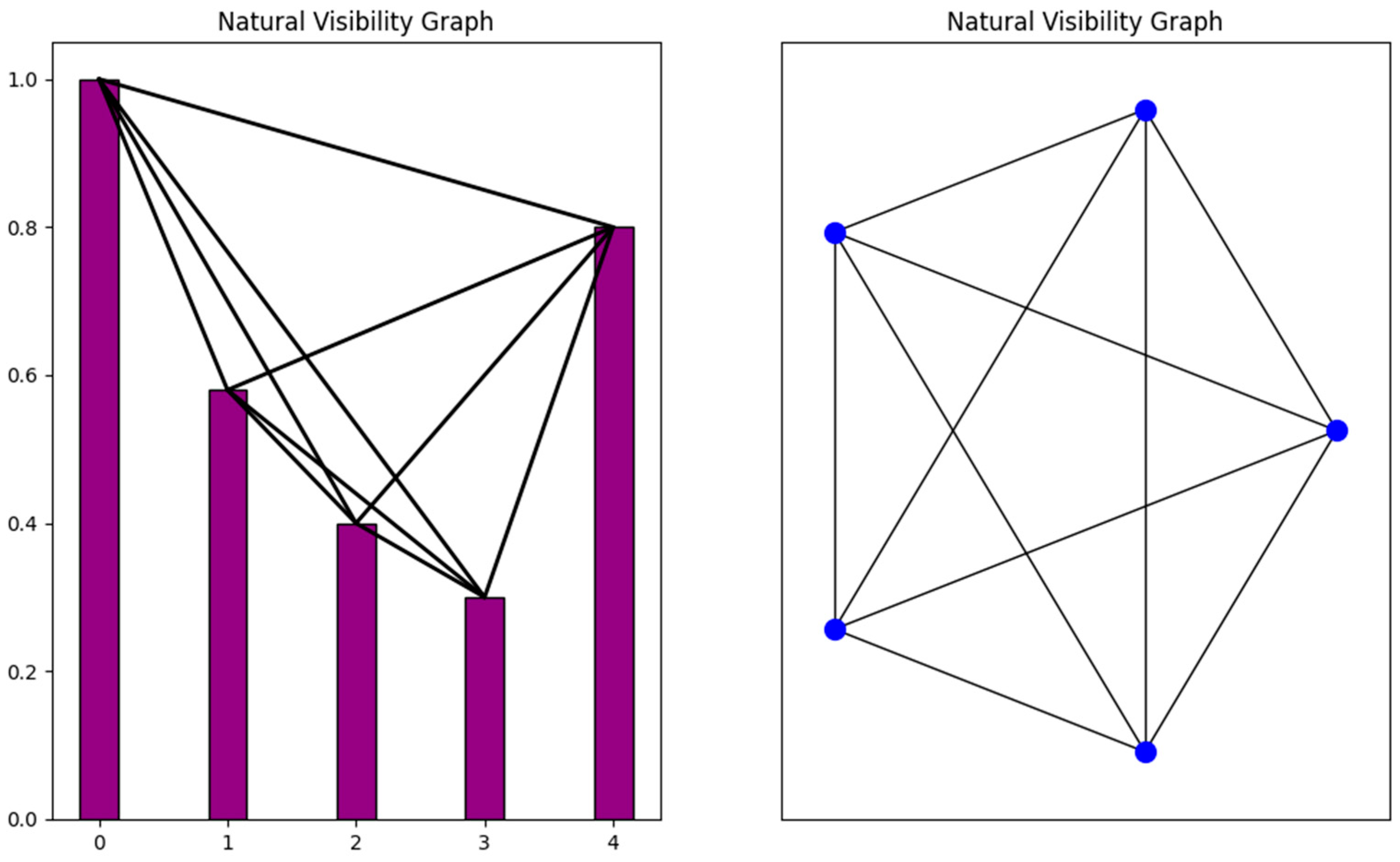
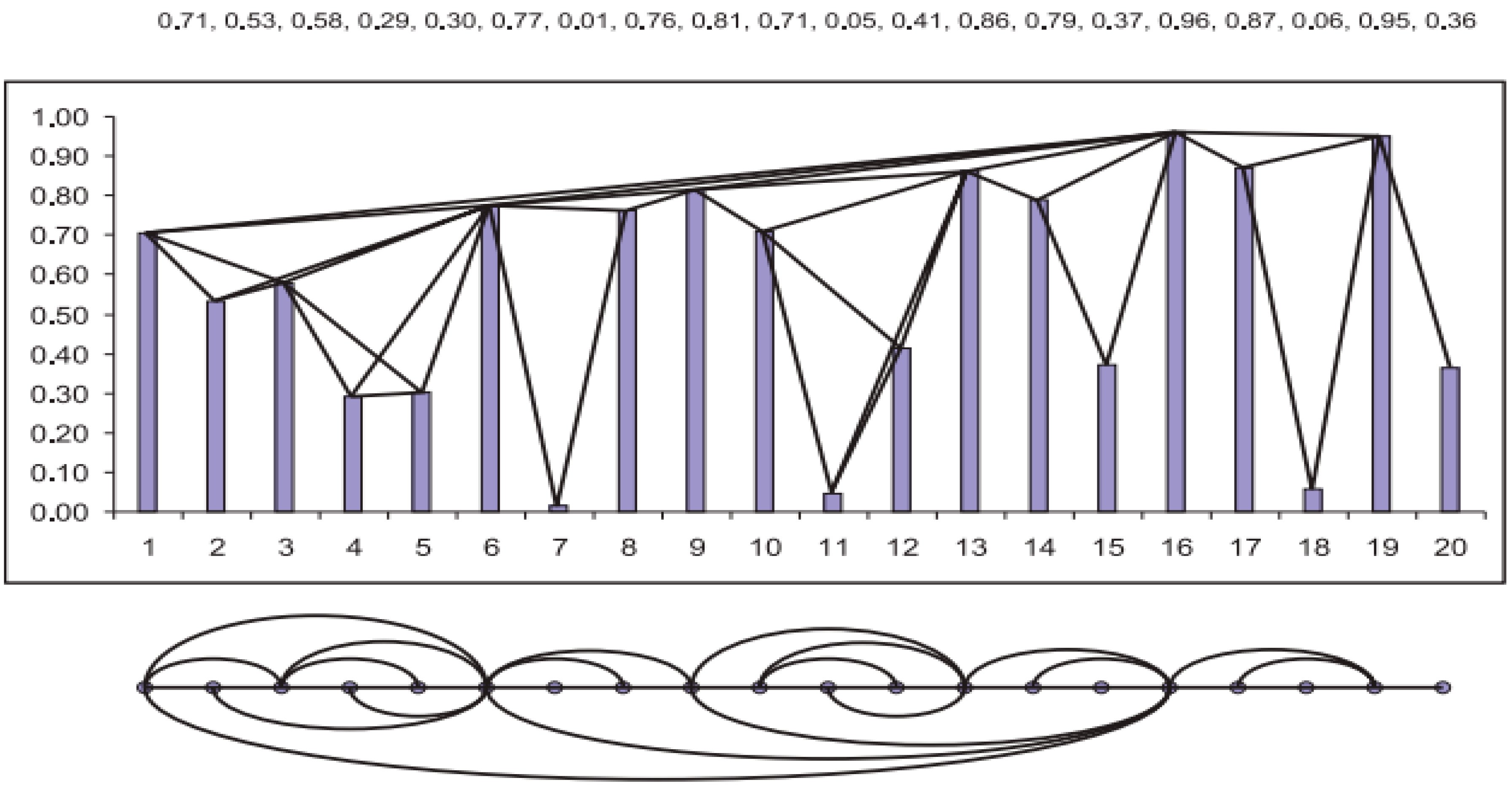
2.1. Visibility Graphs (VG)
2.1.1. Natural Visibility Graph

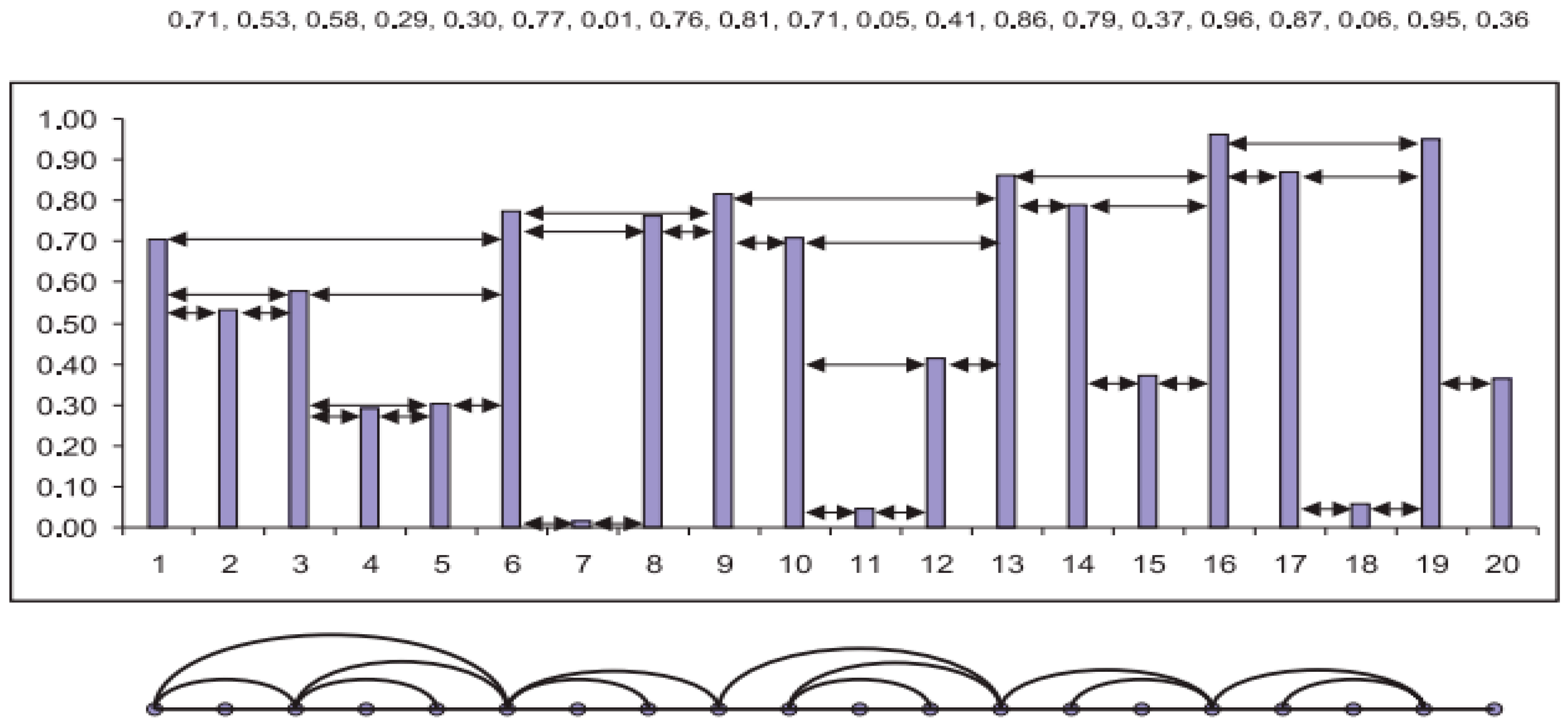
2.1.2. Horizontal Visibility Graph
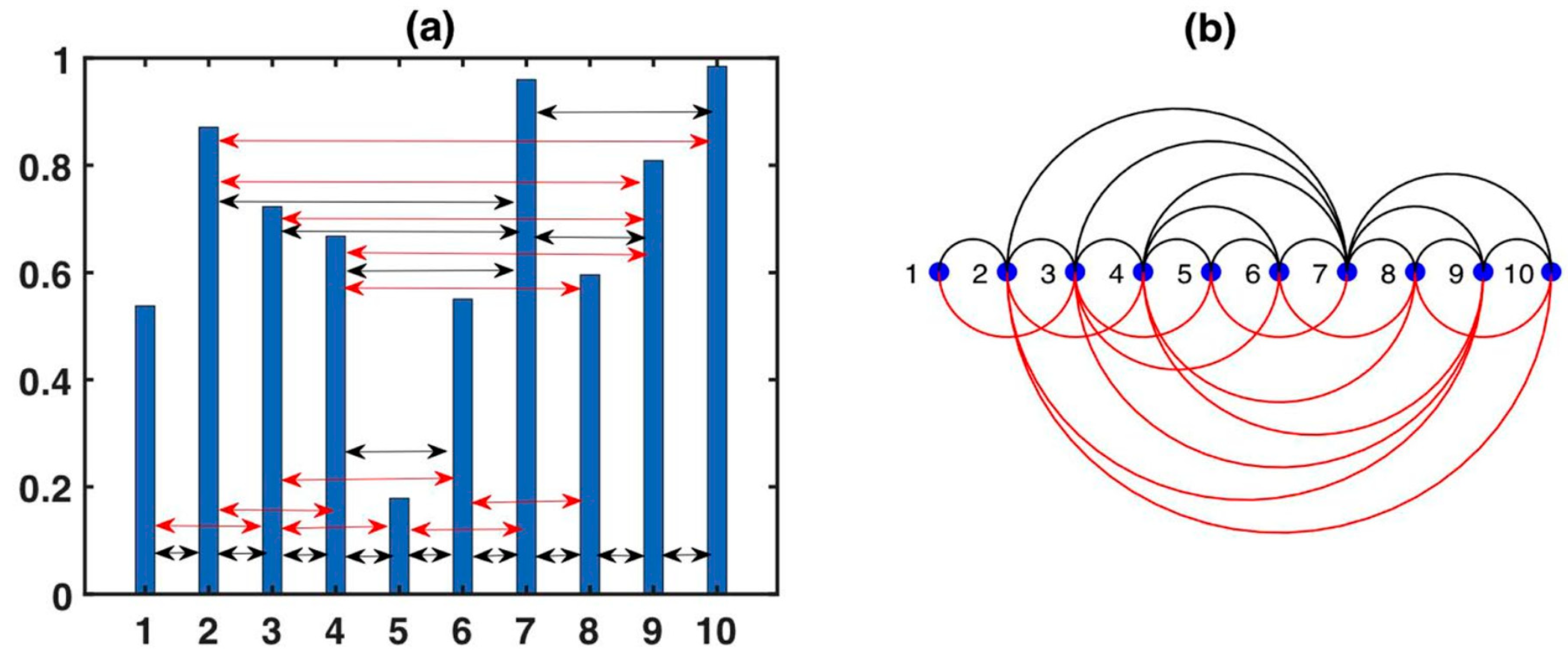
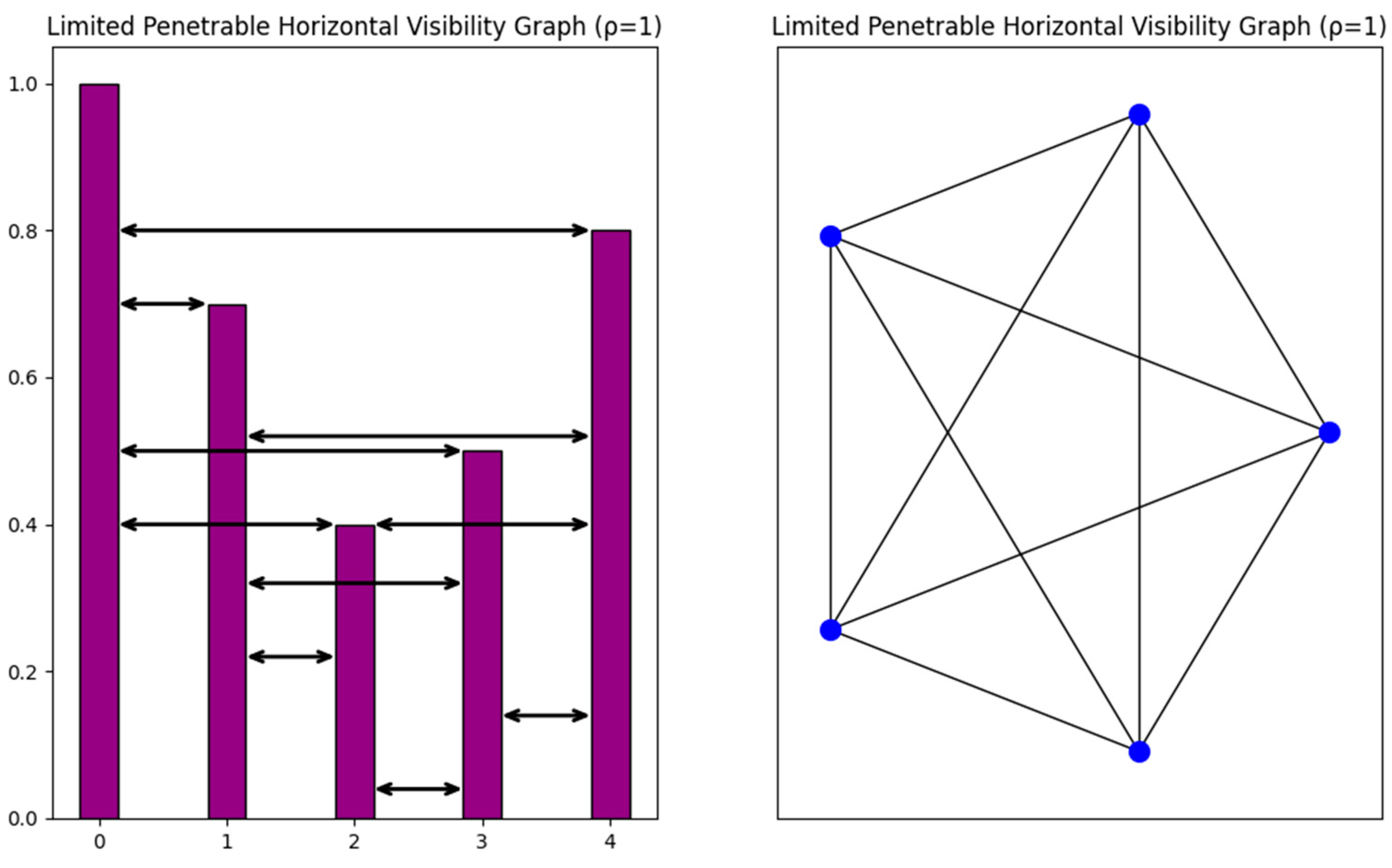
2.1.3. Limited Penetrable Horizontal Visibility Graph
2.2. Phase Space Reconstruction Graphs (PSRG)
3. Signature of Chaos in Networks Associated with Time Series
3.1. Signature of Chaos in Visibility Graphs
3.2. Signature of Chaos in Phase Space Reconstruction Graphs
4. Results
4.1. Results for Torus Automorphisms
4.1.1. Natural Visibility Graph of Torus Automorphisms
4.1.2. Horizontal Visibility Graph of Torus Automorphisms
4.1.3. Limited Penetrable Horizontal Visibility Graph of Torus Automorphisms
4.1.4. Phase Space Reconstruction Graph of Torus Automorphisms
4.2. Results for the Lorenz System
4.2.1. Natural Visibility Graph of the Lorenz System
4.2.2. Horizontal Visibility Graph of the Lorenz System
4.2.3. Limited Penetrable Horizontal Visibility Graph of the Lorenz System
4.2.4. Phase Space Reconstruction Graph of the Lorenz System
4.3. Results for the Random Sequence with Gaussian Distribution
4.3.1. Natural Visibility Graph of the Random Sequence
4.3.2. Horizontal Visibility Graph of the Random Sequence
4.3.3. Limited Penetrable Horizontal Visibility Graph of the Random Sequence
4.3.4. Phase Space Reconstruction of the Random Sequence
5. Meaning of the Results
5.1. Visibility Graphs
5.2. Phase Space Reconstruction Graphs
6. Concluding Remarks
Author Contributions
Funding
Institutional Review Board Statement
Data Availability Statement
Conflicts of Interest
References
- Lorenzelli, F. The Essence of Chaos, 1st ed.; CRC Press: London, UK, 1993. [Google Scholar] [CrossRef]
- Hirsch, M.W.; Smale, S.; Devaney, R.L. Differential Equations, Dynamical Systems, and an Introduction to Chaos, 3rd ed.; Academic Press: Cambridge, MA, USA, 2013. [Google Scholar] [CrossRef]
- Devaney, R.L. An Introduction to Chaotic Dynamical Systems, 3rd ed.; CRC Press: Boca Raton, FL, USA, 2021. [Google Scholar] [CrossRef]
- Hilborn, R.C. Chaos and Nonlinear Dynamics: An Introduction for Scientists and Engineers, 2nd ed.; Oxford University Press: New York, NY, USA, 2000. [Google Scholar] [CrossRef]
- Strogatz, S.H. Nonlinear Dynamics and Chaos: With Applications to Physics, Biology, Chemistry, and Engineering, 2nd ed.; CRC Press: Boca Raton, FL, USA, 2015. [Google Scholar] [CrossRef]
- Cornfeld, I.P.; Fomin, S.V.; Sinai, Y.G. Ergodic Theory, 1st ed.; Springer: New York, NY, USA, 1982. [Google Scholar] [CrossRef]
- Ornstein, D.S.; Weiss, B. Statistical properties of chaotic systems. Bull. Am. Math. Soc. 1991, 24, 11–122. [Google Scholar] [CrossRef]
- Berliner, L. Statistics, Probability and Chaos. Stat. Sci. 1992, 7, 69–90. Available online: https://www.jstor.org/stable/2245991 (accessed on 12 November 2023). [CrossRef]
- Chatterjee, S.; Yilmaz, M.R. Chaos, Fractals and Statistics. Stat. Sci. 1992, 6, 49–121. [Google Scholar] [CrossRef]
- Knuth, D. The Art of Computer Programming, Seminumerical Algorithms, 3rd ed.; Addison-Wesley: Reading, MA, USA, 1997. [Google Scholar]
- Szczepanski, J.; Kotulski, J. Pseudorandom Number Generators Based on Chaotic Dynamical Systems. Open Syst. Inf. Dyn. 2001, 8, 137–146. [Google Scholar] [CrossRef]
- Silva, V.F.; Silva, M.E.; Ribeiro, P.; Silva, F. Novel features for time series analysis: A complex networks approach. Data Min. Knowl. Discov. 2022, 36, 1062–1101. [Google Scholar] [CrossRef]
- Donner, R.V.; Small, M.; Donges, J.F.; Marwan, N.; Zou, Y.; Xiang, R.; Kurths, J. Recurrence-based time series analysis by means of complex network methods. Int. J. Bifurc. Chaos 2011, 21, 1019–1046. [Google Scholar] [CrossRef]
- Zou, Y.; Donner, R.V.; Marwan, N.; Donges, J.F.; Kurths, J. Complex network approaches to nonlinear time series analysis. Phys. Rep. 2019, 787, 1–97. [Google Scholar] [CrossRef]
- Silva, V.F.; Silva, M.E.; Ribeiro, P.; Silva, F. Time Series Analysis via Network Science: Concepts and Algorithms. Wiley Interdiscip. Rev. Data Min. Knowl. Discov. 2021, 11, 1404. [Google Scholar] [CrossRef]
- Lacasa, L.; Toral, R. Description of stochastic and chaotic series using visibility graphs. Phys. Rev. E 2010, 82, 036120. [Google Scholar] [CrossRef]
- Lacasa, L.; Luque, B.; Ballesteros, F.; Luque, J.; Nuno, J.C. From time series to complex networks: The visibility graph. Proc. Natl. Acad. Sci. USA 2008, 105, 4972–4975. [Google Scholar] [CrossRef]
- Provenzale, A.; Smith, L.A.; Vio, R.; Murante, G. Distinguishing between low-dimensional dynamics and randomness in measures time series. Phys. D Nonlinear Phenom. 1992, 58, 31–49. [Google Scholar] [CrossRef]
- Weron, R. Estimating long-range dependence: Finite sample properties and confidence intervals. Phys. A Stat. Mech. Its Appl. 2002, 312, 285–299. [Google Scholar] [CrossRef]
- Hanias, M.; Tsakonas, S.; Magafas, L.; Thalassinos, E.I.; Zachilas, L. Deterministic chaos and forecasting in Amazon? s share prices. Equilib. Q. J. Econ. Econ. Policy 2020, 15, 253–273. [Google Scholar] [CrossRef]
- Stavrinides, S.G.; Hanias, M.P.; Gonzalez, M.B.; Campabadal, F.; Contoyiannis, Y.; Potirakis, S.M.; Al Chawa, M.M.; de Benito, C.; Tetzlaff, R.; Picos, R.; et al. On the chaotic nature of random telegraph noise in unipolar RRAM memristor devices. Chaos Solitons Fractals 2022, 160, 112224. [Google Scholar] [CrossRef]
- Gao, Z.; Jin, N. Complex network from time series based on phase space reconstruction. Chaos 2009, 19, 033137. [Google Scholar] [CrossRef] [PubMed]
- Nuñez, A.M.; Lacasa, L.; Patricio, J.; Luque, B. Visibility Algorithms: A Short Review. In New Frontiers in Graph Theory; BoD—Books on Demand: Norderstedt, Germany, 2012; pp. 119–152. [Google Scholar] [CrossRef]
- Mira-Iglesias, A.; Navarro-Pardo, E.; Conejero, J.A. Power-Law Distribution of Natural Visibility Graphs from Reaction Times Series. Symmetry 2019, 11, 563. [Google Scholar] [CrossRef]
- Xu, P.; Zhang, R.; Deng, Y. A novel visibility graph transformation of time series into weighted networks. Chaos Solitons Fractals 2018, 117, 201–208. [Google Scholar] [CrossRef]
- Wang, N.; Li, D.; Wang, Q. Visibility graph analysis on quarterly macroeconomic series of China based on complex network theory. Phys. A Stat. Mech. Its Appl. 2012, 391, 6543–6555. [Google Scholar] [CrossRef]
- Qian, M.-C.; Jiang, Z.-Q.; Zhou, W.-X. Universal and nonuniversal allometric scaling behaviors in the visibility graphs of world stock market indices. J. Phys. A Math. Theor. 2010, 43, 335002. [Google Scholar] [CrossRef]
- Sun, M.; Wang, Y.; Gao, C. Visibility graph network analysis of natural gas price: The case of North American market. Phys. A Stat. Mech. Its Appl. 2016, 462, 1–11. [Google Scholar] [CrossRef]
- Donner, R.V.; Donges, J.F. Visibility graph analysis of geophysical time series: Potentials and possible pitfalls. Acta Geophys. 2012, 60, 589–623. [Google Scholar] [CrossRef]
- Stephen, M.; Gu, C.; Yang, H. Visibility Graph Based Time Series Analysis. PLoS ONE 2015, 10, e0143015. [Google Scholar] [CrossRef]
- Telesca, L.; Lovallo, M. Analysis of seismic sequences by using the method of visibility graph. Europhys. Lett. 2012, 97, 50002. [Google Scholar] [CrossRef]
- Tang, J.; Liu, F.; Zhang, W.; Zhang, S.; Wang, Y. Exploring dynamic property of traffic flow time series in multi-states based on complex networks: Phase space reconstruction versus visibility graph. Phys. A Stat. Mech. Its Appl. 2016, 450, 635–648. [Google Scholar] [CrossRef]
- Baggio, R.; Sainaghi, R. Mapping time series into networks as a tool to assess the complex dynamics of tourism systems. Tour. Manag. 2016, 54, 23–33. [Google Scholar] [CrossRef]
- Ahmadlou, M.; Adeli, H.; Adeli, A. New diagnostic EEG markers of the Alzheimer’s disease using visibility graph. J. Neural Transm. 2010, 117, 1099–1109. [Google Scholar] [CrossRef]
- Ahmadlou, M.; Adeli, H.; Adeli, A. Improved visibility graph fractality with application for the diagnosis of Autism Spectrum Disorder. Phys. A Stat. Mech. Its Appl. 2012, 391, 4720–4726. [Google Scholar] [CrossRef]
- Hou, F.Z.; Li, F.W.; Wang, J.; Yan, F.R. Visibility graph analysis of very short-term heart rate variability during sleep. Phys. A Stat. Mech. Its Appl. 2016, 458, 140–145. [Google Scholar] [CrossRef]
- Lacasa, L.; Flanagan, R. Time reversibility from visibility graphs of nonstationary processes. Phys. Rev. E 2015, 92, 022817. [Google Scholar] [CrossRef]
- Iacovacci, J.; Lacasa, L. Sequential visibility-graph motifs. Phys. Rev. E 2016, 93, 042309. [Google Scholar] [CrossRef]
- Iacovacci, J.; Lacasa, L. Sequential motif profile of natural visibility graphs. Phys. Rev. E 2016, 94, 052309. [Google Scholar] [CrossRef]
- Rahman, M.S. Basic Graph Theory, 1st ed.; Planar Graphs; Springer: Cham, Switzerland, 2017; pp. 77–89. [Google Scholar] [CrossRef]
- Kuratowski, K. Sur le probleme des courbes gauches en topologie. Fundam. Math. 1930, 15, 271–283. [Google Scholar] [CrossRef]
- Luque, B.; Lacasa, L.; Ballesteros, F.; Luque, J. Horizontal visibility graphs: Exact results for random time series. Phys. Rev. E 2009, 80, 046103. [Google Scholar] [CrossRef]
- Gao, Z.K.; Cai, Q.; Yang, Y.X.; Dang, W.D.; Zhang, S.S. Multiscale limited penetrable horizontal visibility graph for analyzing nonlinear time series. Sci. Rep. 2016, 6, 35622. [Google Scholar] [CrossRef]
- Wang, M.; Vilela, A.L.M.; Du, R.; Zhao, L.; Dong, G.; Tian, L.; Stanley, H.E. Exact results of the limited penetrable horizontal visibility graph associated to random time series and its application. Sci. Rep. 2018, 8, 5130. [Google Scholar] [CrossRef]
- Hu, X.; Niu, M. Degree distributions and motif profiles of Thue–Morse complex network. Chaos Solitons Fractals 2023, 176, 114141. [Google Scholar] [CrossRef]
- Cai, Q.; Gao, Z.K.; Yang, Y.X.; Dang, W.D.; Grebogi, C. Multiplex Limited Penetrable Horizontal Visibility Graph from EEG Signals for Driver Fatigue Detection. Int. J. Neural Syst. 2019, 29, 1850057. [Google Scholar] [CrossRef]
- Wang, M.; Vilela, A.L.M.; Du, R.; Zhao, L.; Dong, G.; Tian, L.; Stanley, H.E. Topological properties of the limited penetrable horizontal visibility graph family. Phys. Rev. E 2018, 97, 052117. [Google Scholar] [CrossRef]
- Gutin, G.; Mansour, T.; Severini, S. A characterization of horizontal visibility graphs and combinatorics on words. Phys. A Stat. Mech. Its Appl. 2011, 390, 2421–2428. [Google Scholar] [CrossRef]
- Taken, F. Dynamical Systems and Turbulence; Lecture Notes in Mathematics; Springer: Berlin/Heidelberg, Germany, 1981; p. 898. [Google Scholar] [CrossRef]
- Ravetti, M.G.; Carpi, L.C.; Gonçalves, B.A.; Frery, A.C.; Rosso, O.A. Distinguishing Noise from Chaos: Objective versus Subjective Criteria Using Horizontal Visibility Graph. PLoS ONE 2014, 9, e108004. [Google Scholar] [CrossRef]
- Zhang, R.; Zou, Y.; Zhou, J.; Gao, Z.-K.; Guan, S. Visibility graph analysis for re-sampled time series from auto-regressive stochastic processes. Commun. Nonlinear Sci. Numer. Simul. 2017, 42, 396–403. [Google Scholar] [CrossRef]
- Acosta-Tripailao, B.; Pastén, D.; Moya, P.S. Applying the Horizontal Visibility Graph Method to Study Irreversibility of Electromagnetic Turbulence in Non-Thermal Plasmas. Entropy 2021, 23, 470. [Google Scholar] [CrossRef]
- Ghimire, G.R.; Jadidoleslam, N.; Krajewski, W.F.; Tsonis, A.A. Insights on Streamflow Predictability Across Scales Using Horizontal Visibility Graph Based Networks. Front. Water 2020, 2, 17. [Google Scholar] [CrossRef]
- Zhang, Z.; Zhang, A.; Sun, C.; Xiang, S.; Li, S. Data-Driven Analysis of the Chaotic Characteristics of Air Traffic Flow. J. Adv. Transp. 2020, 2020, 17. [Google Scholar] [CrossRef]
- Provenzano, D.; Baggio, R. Complexity traits and synchrony of cryptocurrencies price dynamics. Decis. Econ. Financ. 2020, 44, 941–955. [Google Scholar] [CrossRef]
- Gómez-Gómez, J.; Carmona-Cabezas, R.; Sánchez-López, E.; Gutiérrez de Ravé, E.; Jiménez-Hornero, F.J. Analysis of Air Mean Temperature Anomalies by Using Horizontal Visibility Graphs. Entropy 2021, 23, 207. [Google Scholar] [CrossRef]
- Wang, M.; Tian, L. From time series to complex networks: The phase space coarse graining. Phys. A Stat. Mech. Its Appl. 2016, 461, 456–468. [Google Scholar] [CrossRef]
- Kennel, M.B.; Brown, R.; Abarbanel, H.D. Determining embedding dimension for phase-space reconstruction using a geometrical construction. Phys. Rev. A At. Mol. Opt. Phys. 1992, 45, 3403–3411. [Google Scholar] [CrossRef]
- Cao, L. Practical method for determining the minimum embedding dimension of a scalar time series. Phys. D Nonlinear Phenom. 1997, 110, 43–50. [Google Scholar] [CrossRef]
- Makris, G.; Antoniou, I. Chaos Cryptography: Relation Of Entropy with Message Length and Period. Chaotic Model. Simul. (CMSIM)-Proofs 2013, 4, 571–581. [Google Scholar]
- Bashkirov, A.G.; Vityazev, A.V. Information entropy and power-law distributions for chaotic systems. Phys. A Stat. Mech. Its Appl. 2000, 277, 136–145. [Google Scholar] [CrossRef]


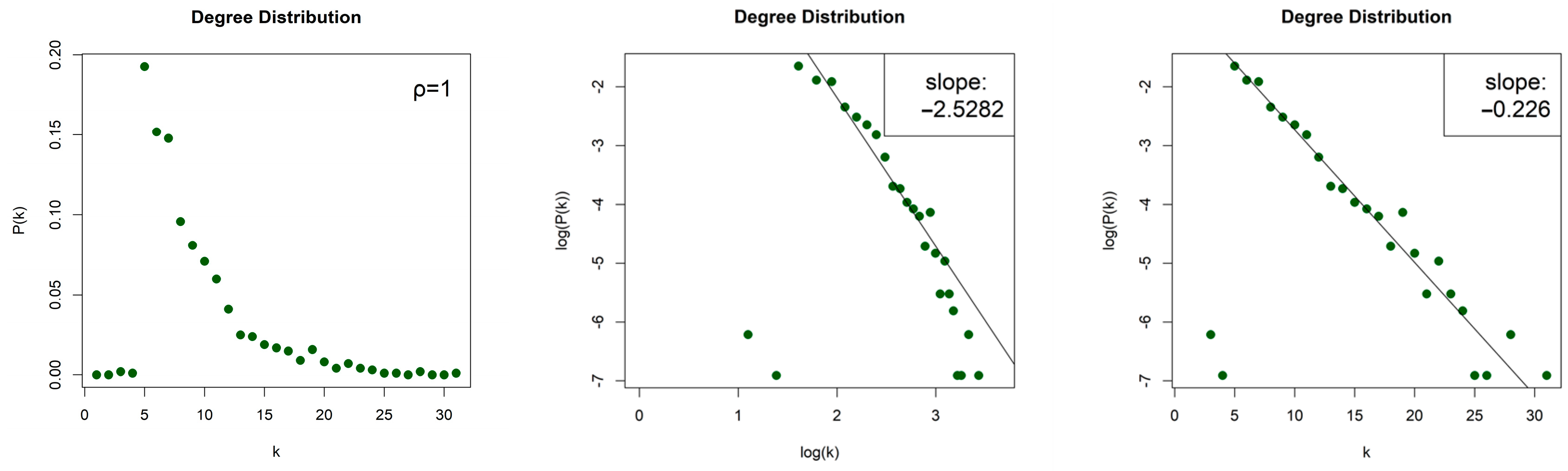
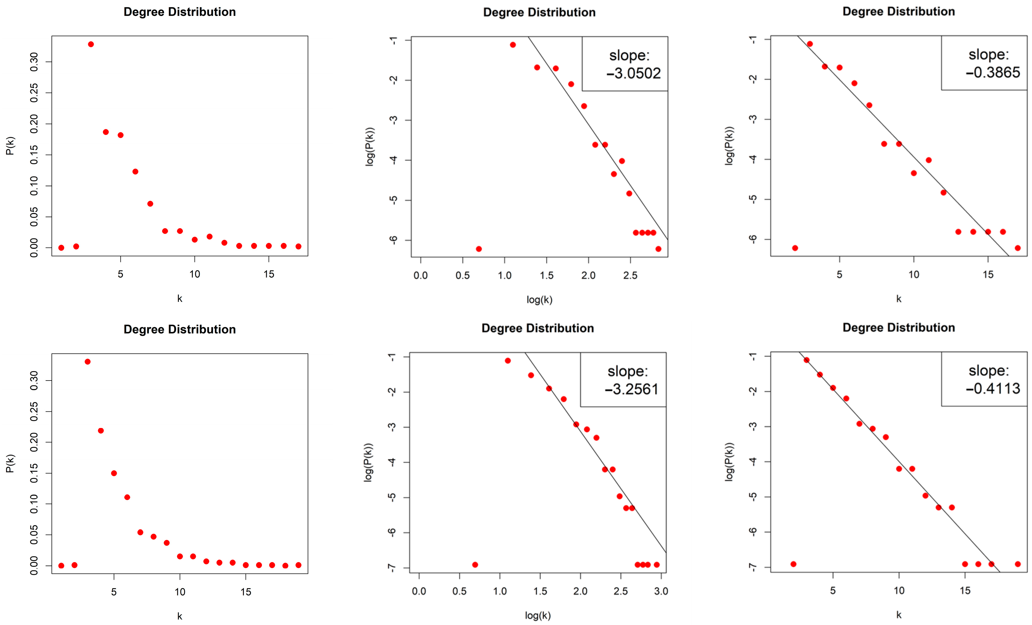
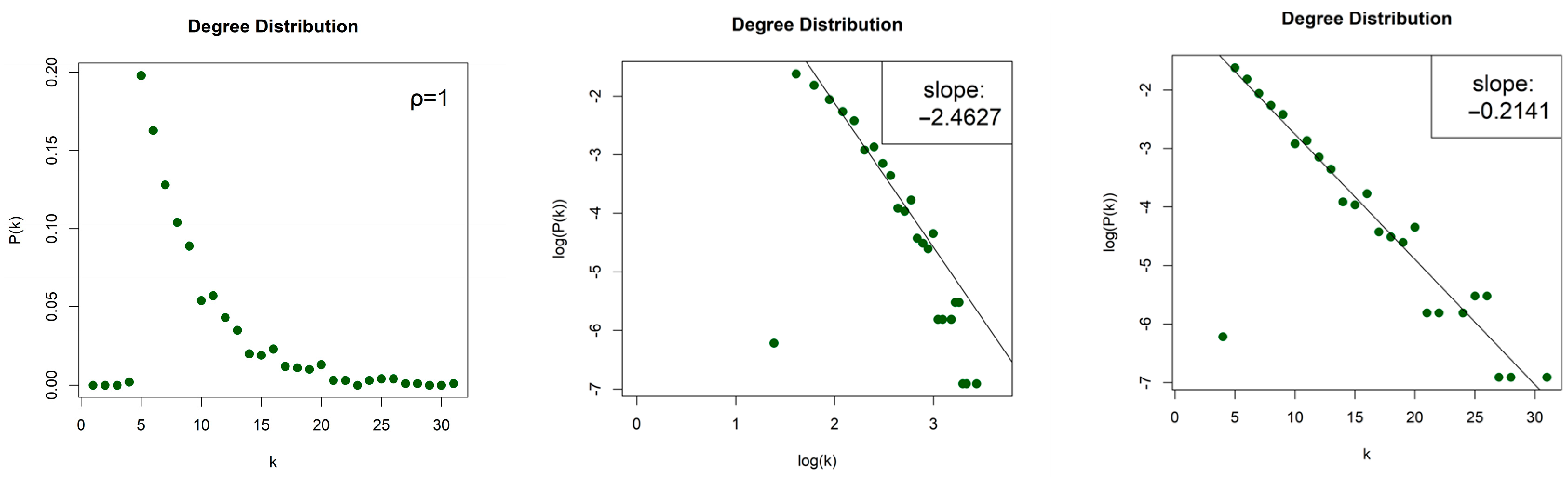
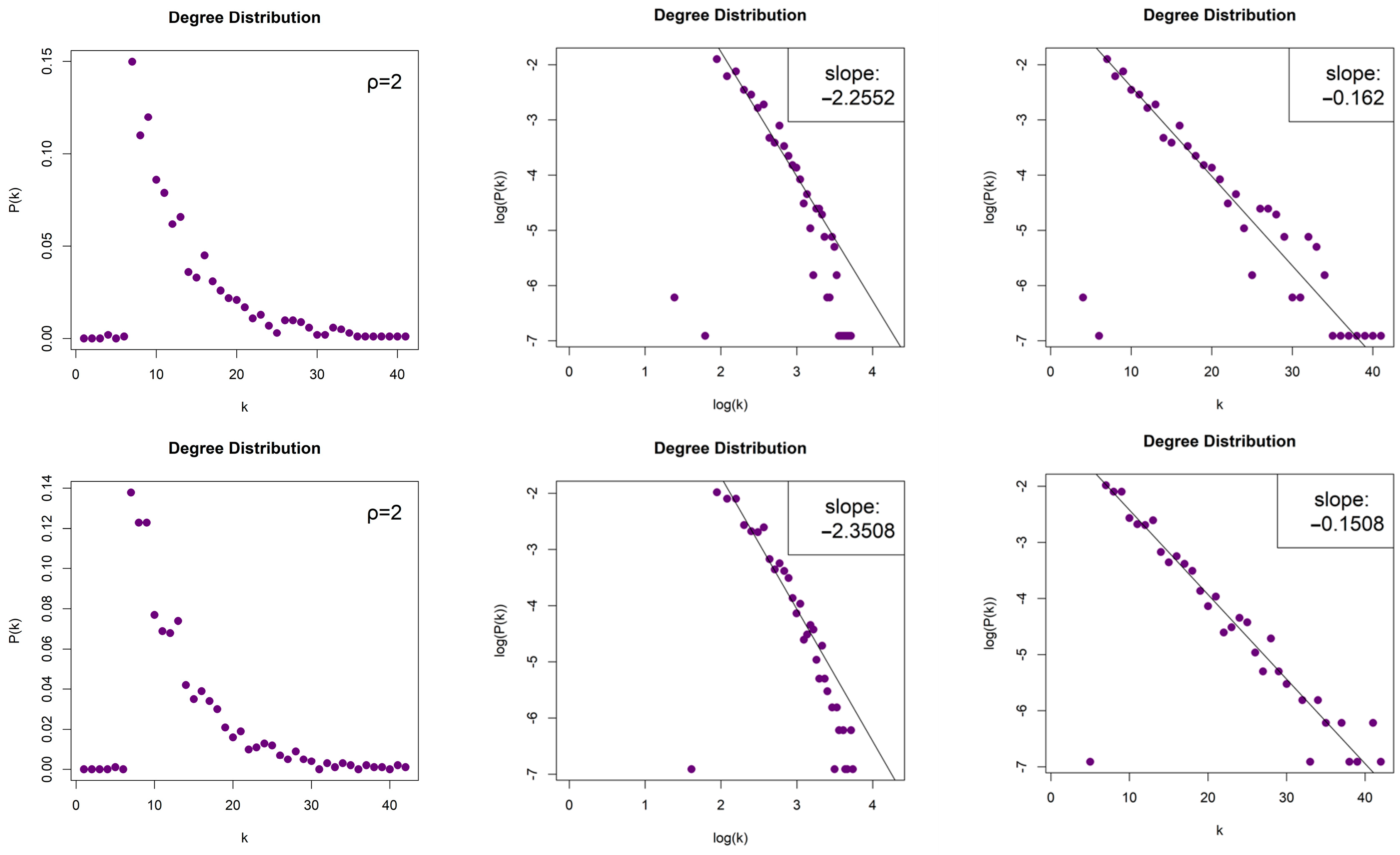
| Time Series Source | NVG Power|Exp log–log|lin–log | HVG Power|Exp log–log|lin–log | LPHVG (ρ = 1) Power|Exp log–log|lin–log | LPHVG (ρ = 2) Power|Exp log–log|lin–log |
|---|---|---|---|---|
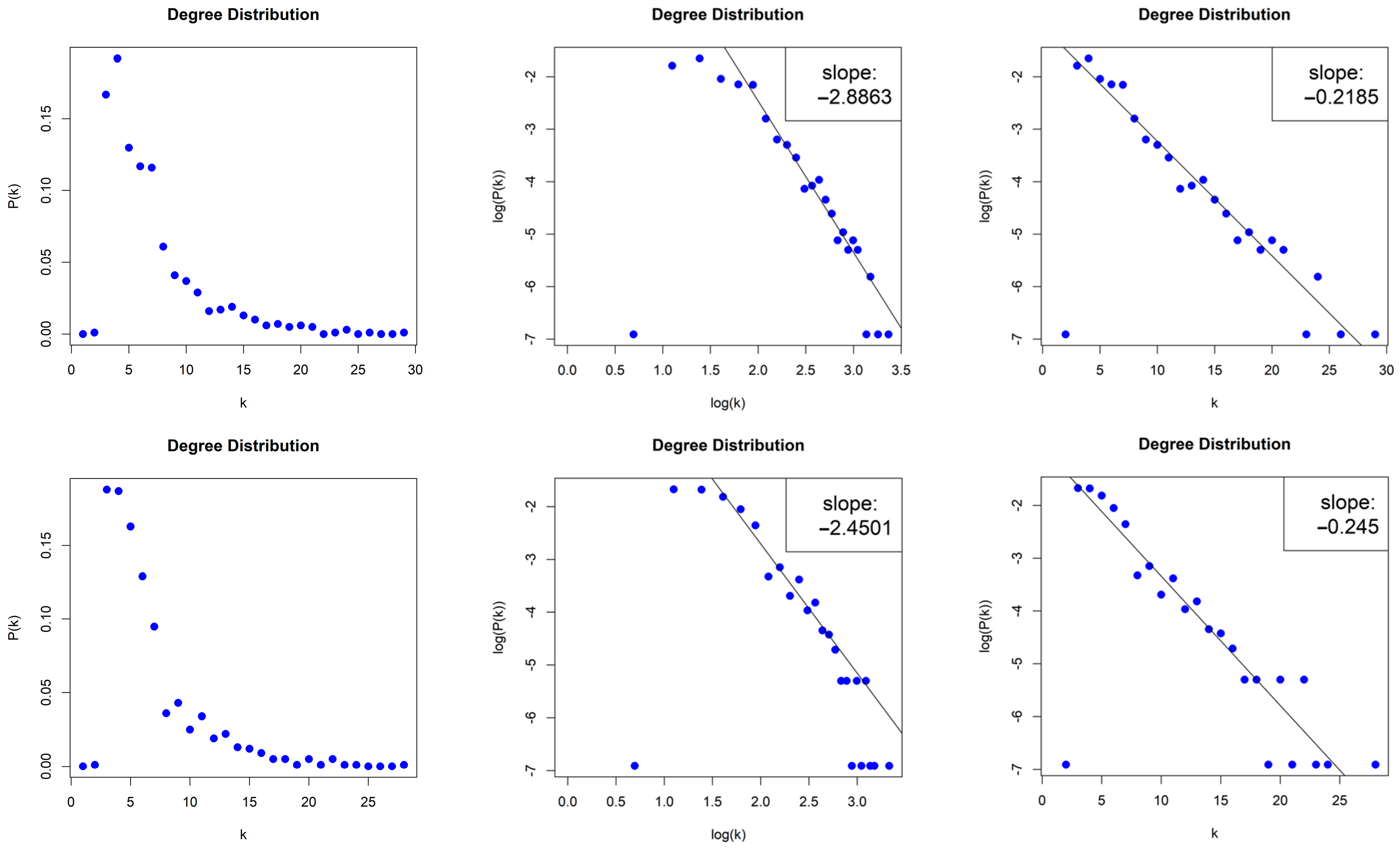
| −2.8863|−0.2185 | −3.0502|−0.3865 | −2.5282|−0.2260 | −2.2552|−0.1620 | |
| −2.4501|−0.2450 | −3.2561|−0.4113 | −2.4627|−0.2141 | −2.3508|−0.1508 | |
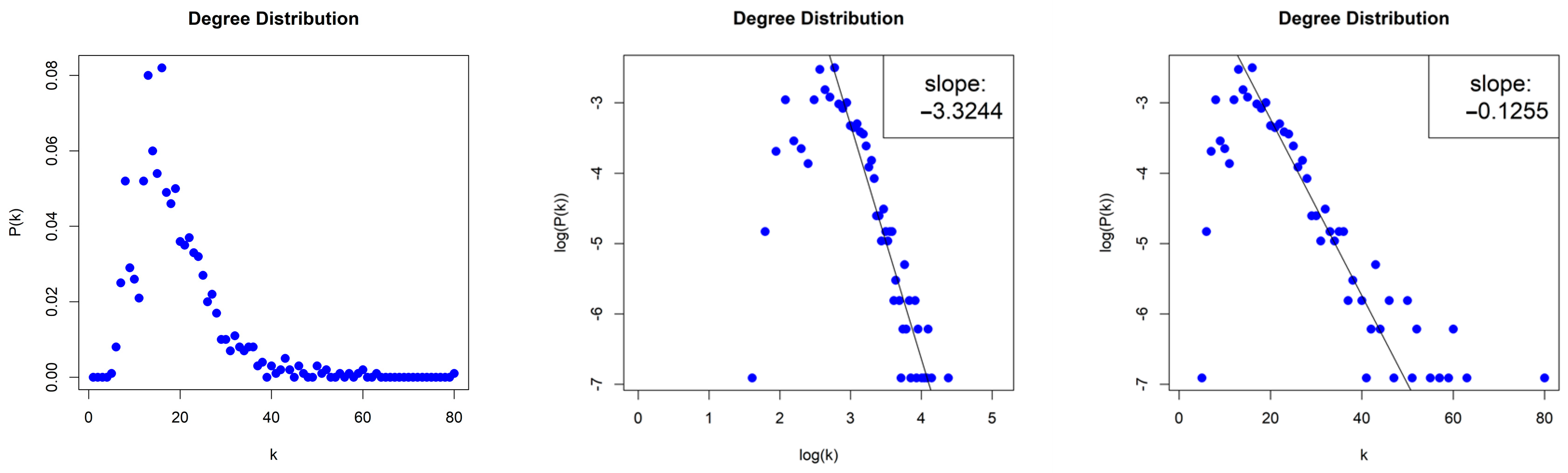
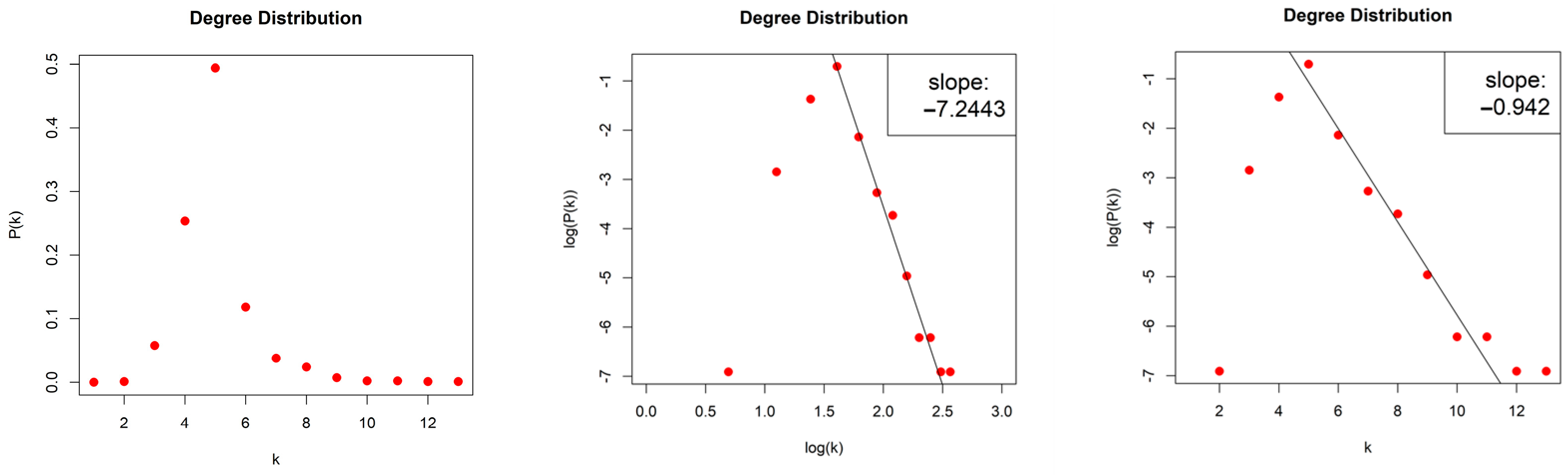
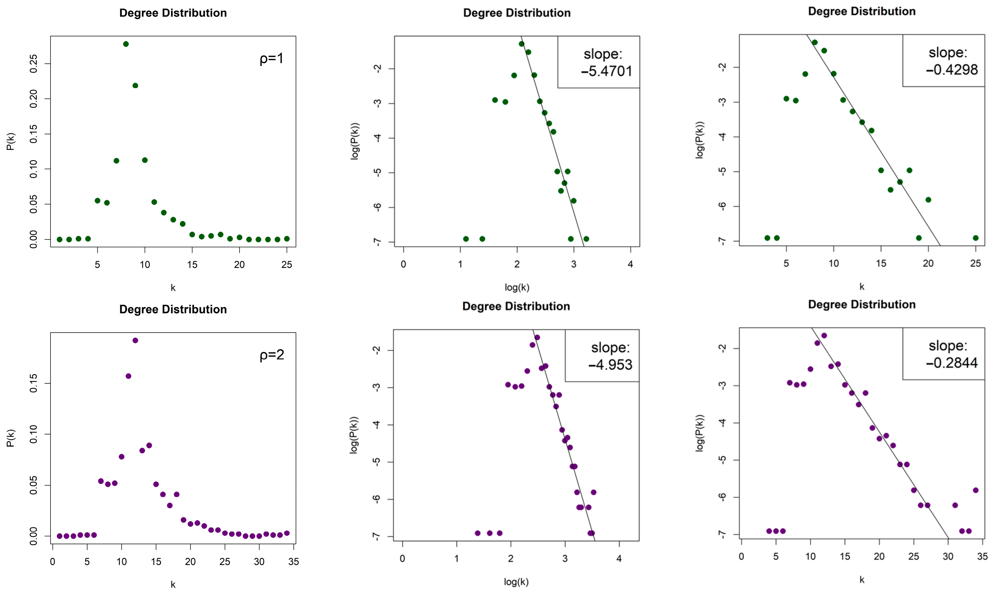
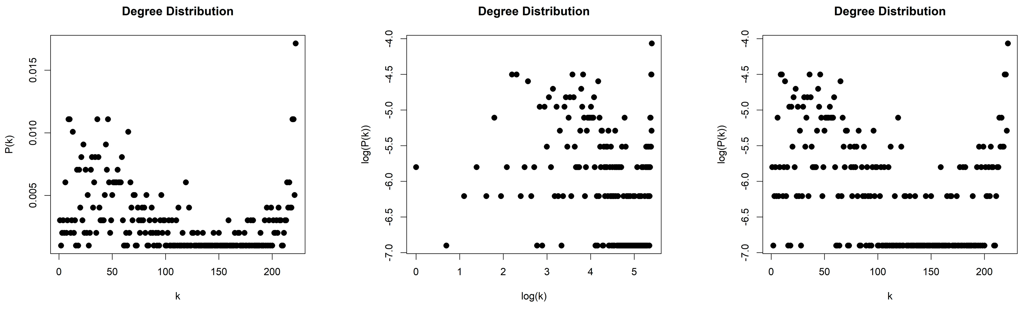
| Lorenz System | −3.3244|−0.1255 | −7.2443|−0.9420 | −5.4701|−0.4298 | −4.9530|−0.2844 |
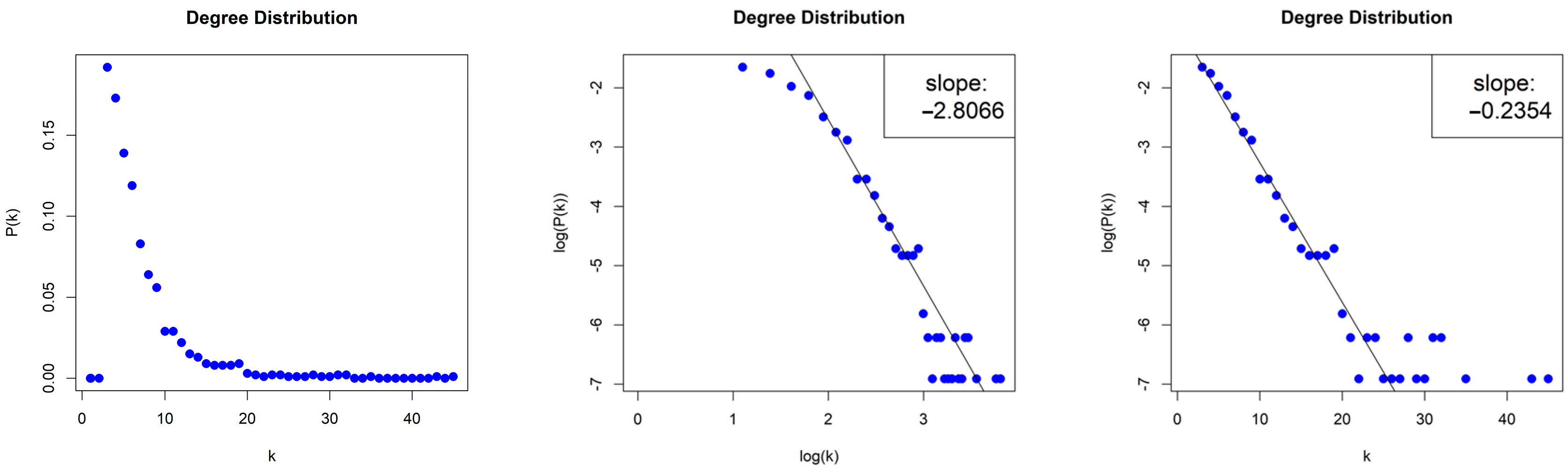
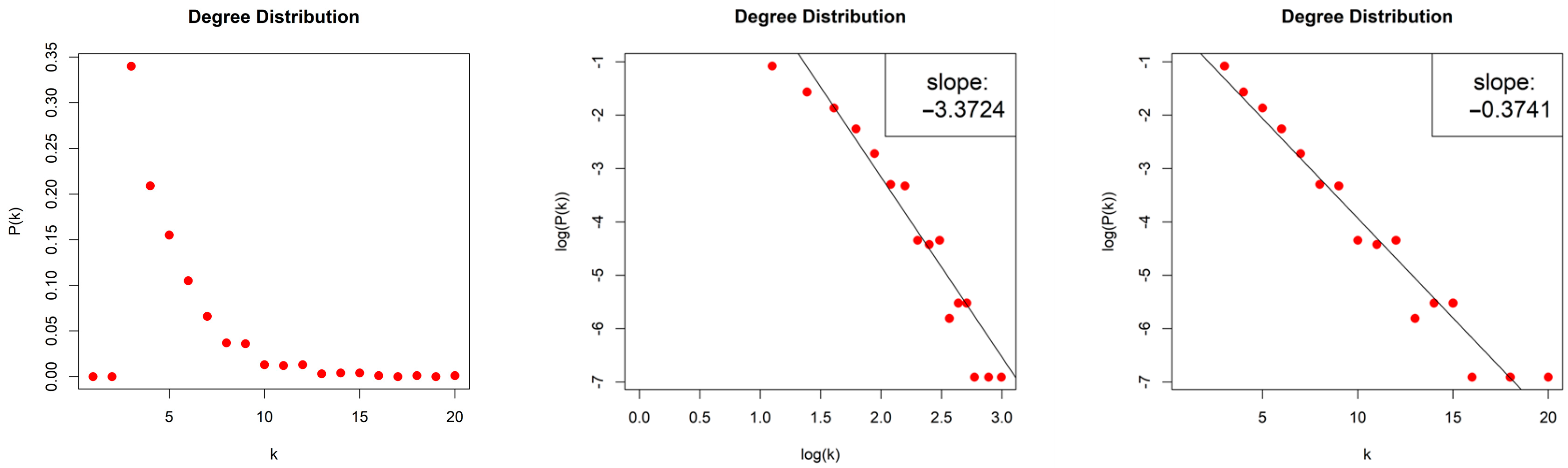
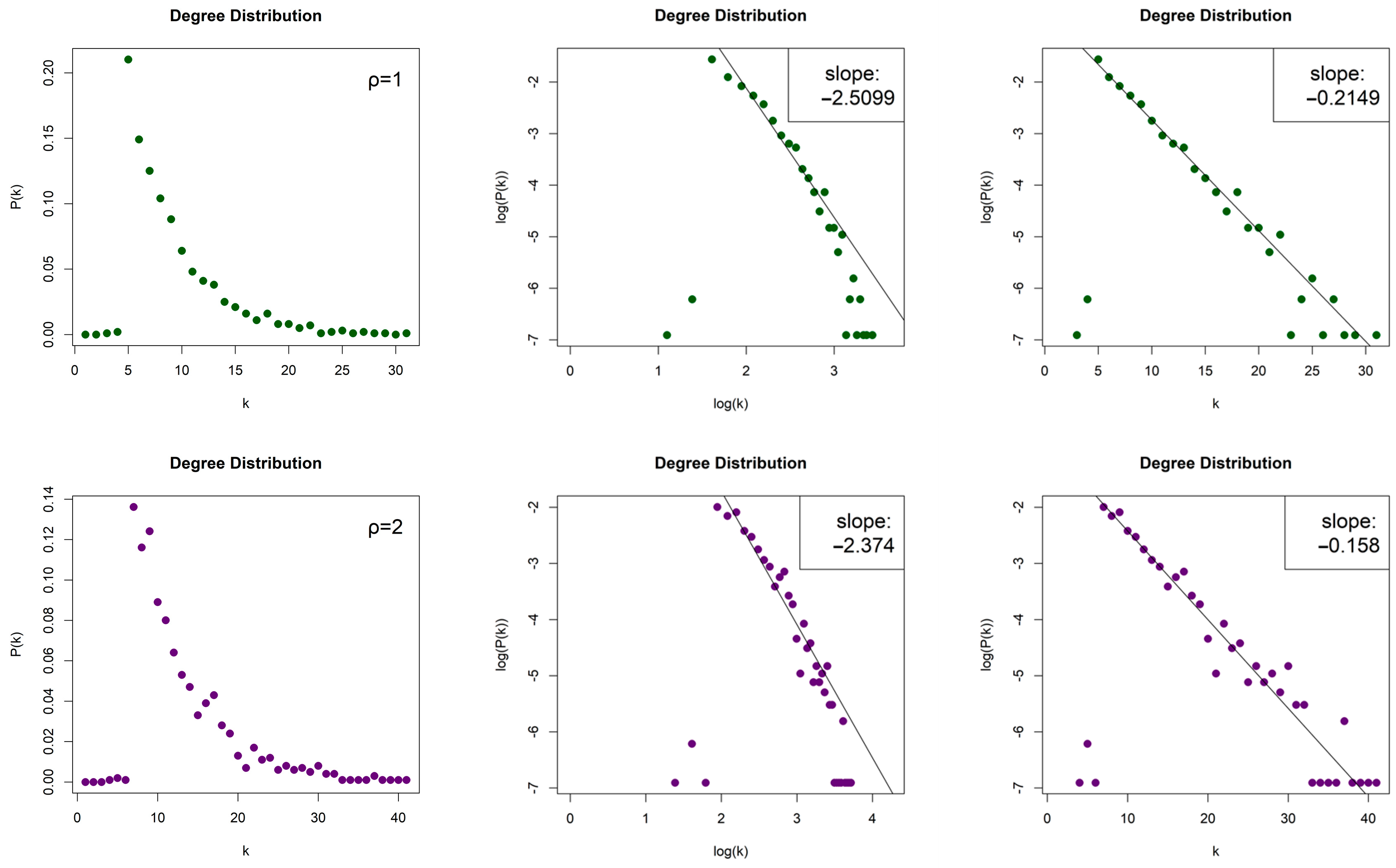
| Random Sequence | −2.8066|−0.2354 | −3.3724|−0.3741 | −2.5099|−0.2149 | −2.3740|−0.1580 |
Disclaimer/Publisher’s Note: The statements, opinions and data contained in all publications are solely those of the individual author(s) and contributor(s) and not of MDPI and/or the editor(s). MDPI and/or the editor(s) disclaim responsibility for any injury to people or property resulting from any ideas, methods, instructions or products referred to in the content. |
© 2024 by the authors. Licensee MDPI, Basel, Switzerland. This article is an open access article distributed under the terms and conditions of the Creative Commons Attribution (CC BY) license (https://creativecommons.org/licenses/by/4.0/).
Share and Cite
Angelidis, A.K.; Goulas, K.; Bratsas, C.; Makris, G.C.; Hanias, M.P.; Stavrinides, S.G.; Antoniou, I.E. Distinction of Chaos from Randomness Is Not Possible from the Degree Distribution of the Visibility and Phase Space Reconstruction Graphs. Entropy 2024, 26, 341. https://doi.org/10.3390/e26040341
Angelidis AK, Goulas K, Bratsas C, Makris GC, Hanias MP, Stavrinides SG, Antoniou IE. Distinction of Chaos from Randomness Is Not Possible from the Degree Distribution of the Visibility and Phase Space Reconstruction Graphs. Entropy. 2024; 26(4):341. https://doi.org/10.3390/e26040341
Chicago/Turabian StyleAngelidis, Alexandros K., Konstantinos Goulas, Charalampos Bratsas, Georgios C. Makris, Michael P. Hanias, Stavros G. Stavrinides, and Ioannis E. Antoniou. 2024. "Distinction of Chaos from Randomness Is Not Possible from the Degree Distribution of the Visibility and Phase Space Reconstruction Graphs" Entropy 26, no. 4: 341. https://doi.org/10.3390/e26040341
APA StyleAngelidis, A. K., Goulas, K., Bratsas, C., Makris, G. C., Hanias, M. P., Stavrinides, S. G., & Antoniou, I. E. (2024). Distinction of Chaos from Randomness Is Not Possible from the Degree Distribution of the Visibility and Phase Space Reconstruction Graphs. Entropy, 26(4), 341. https://doi.org/10.3390/e26040341