
Rise and Fall of Anderson Localization by Lattice Vibrations: A Time-Dependent Machine Learning Approach


Abstract
1. Introduction
2. Theory and Methods
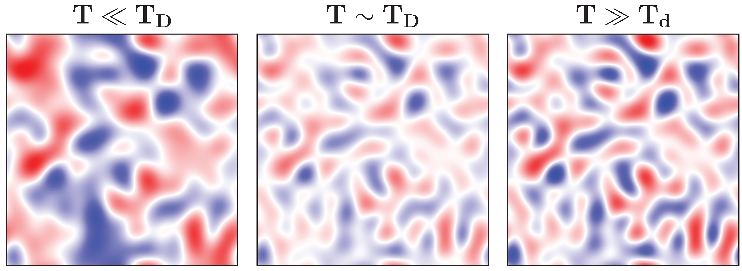
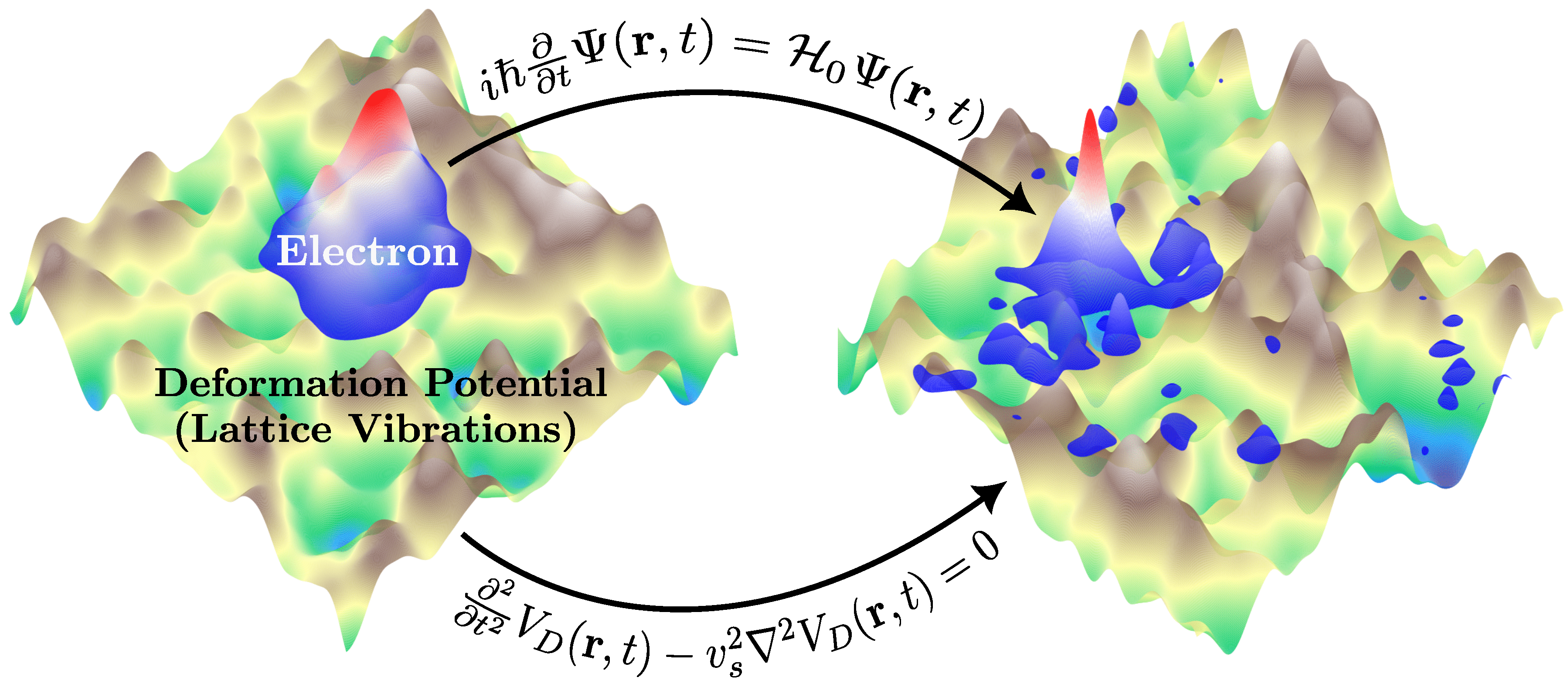
2.1. Deformation Potential
2.2. Electron Dynamics
2.3. Clustering
3. Results
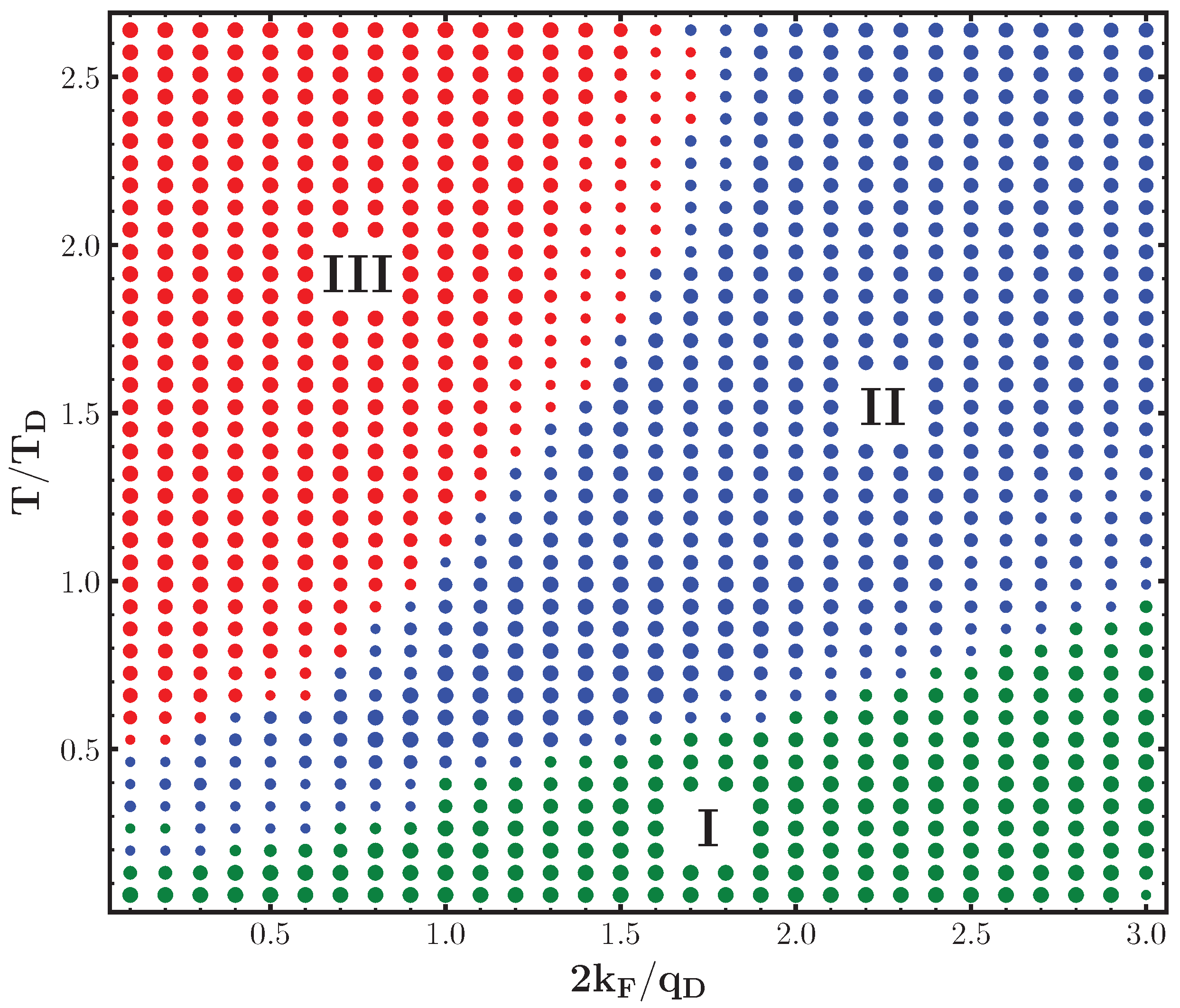
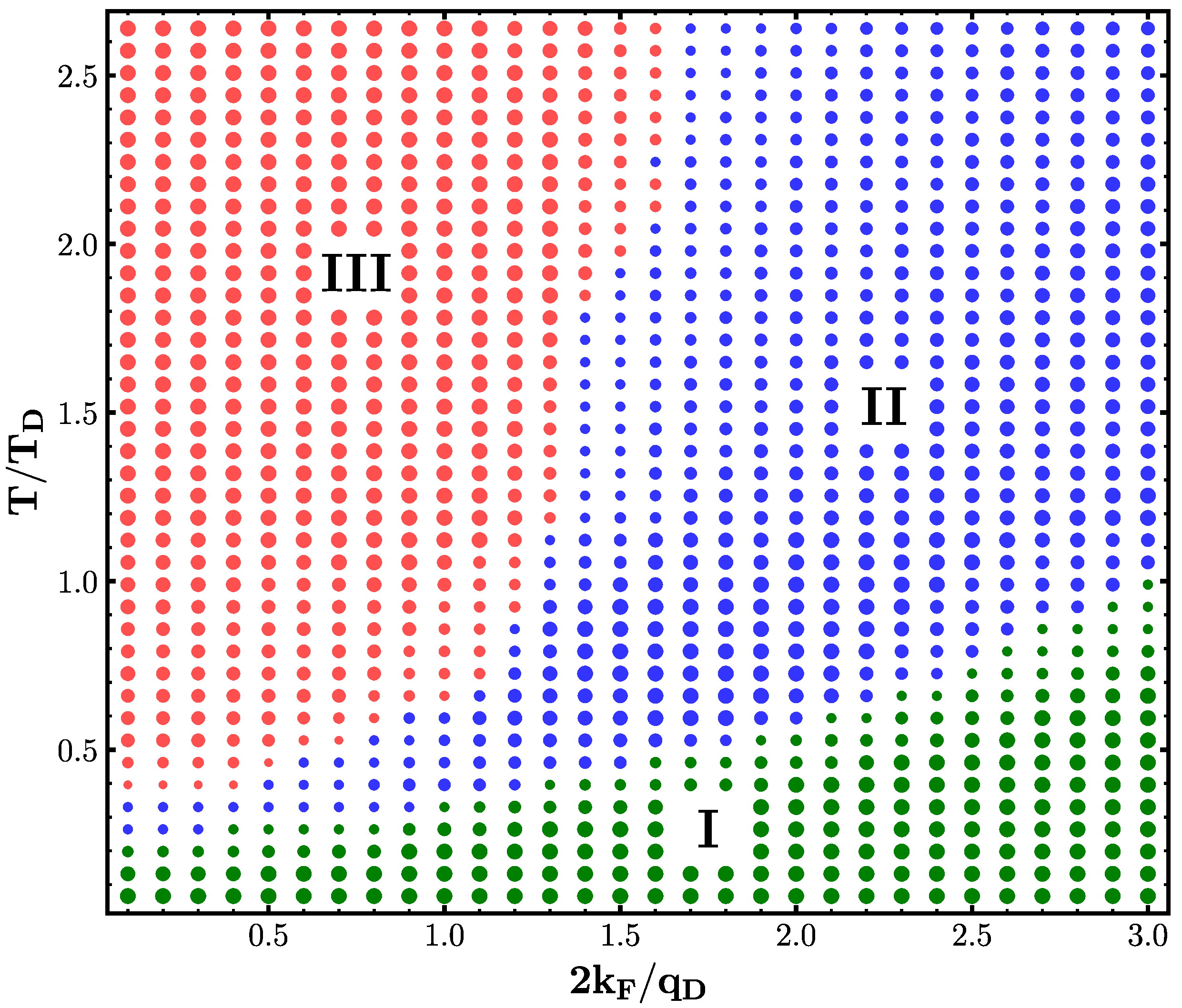
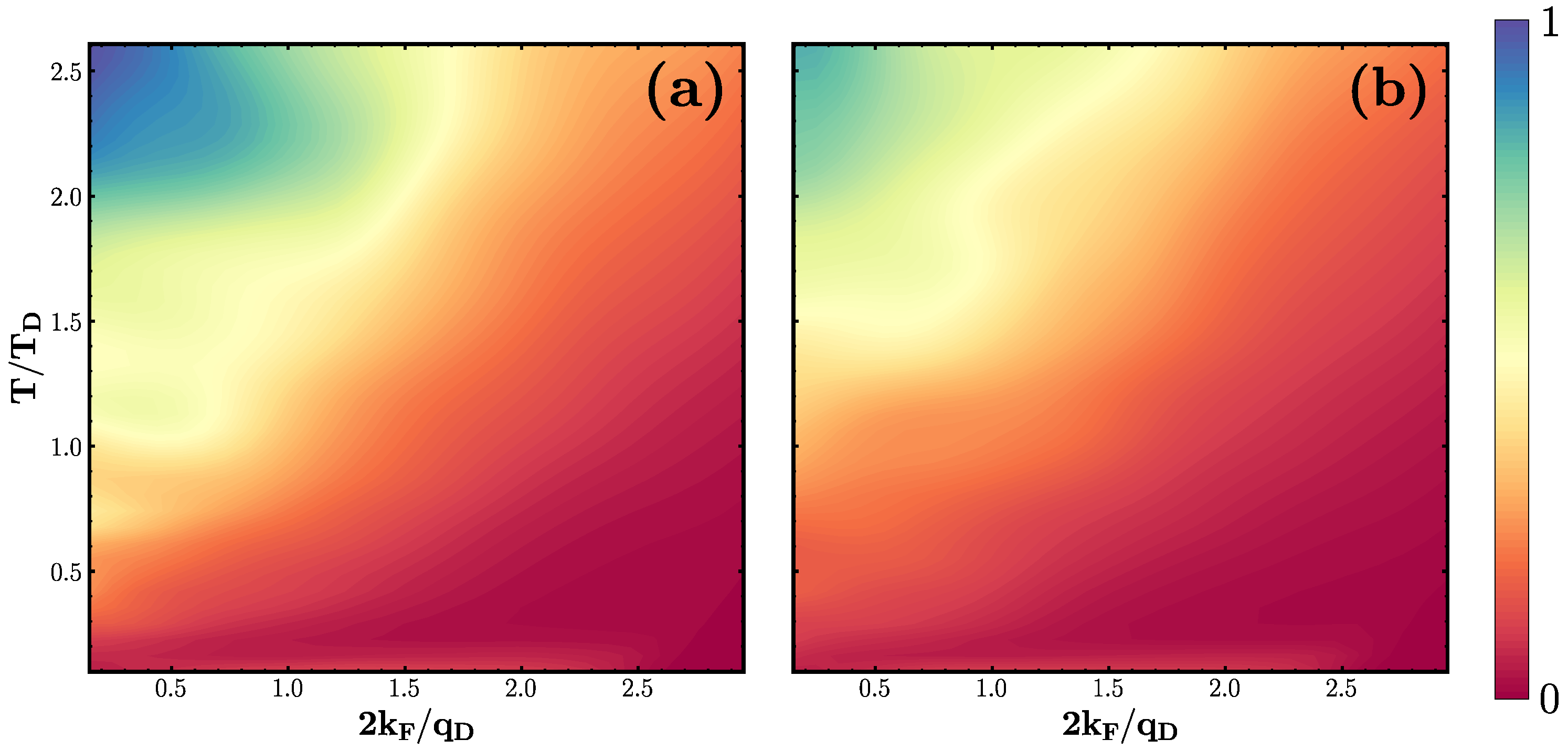
3.1. Phase Diagram
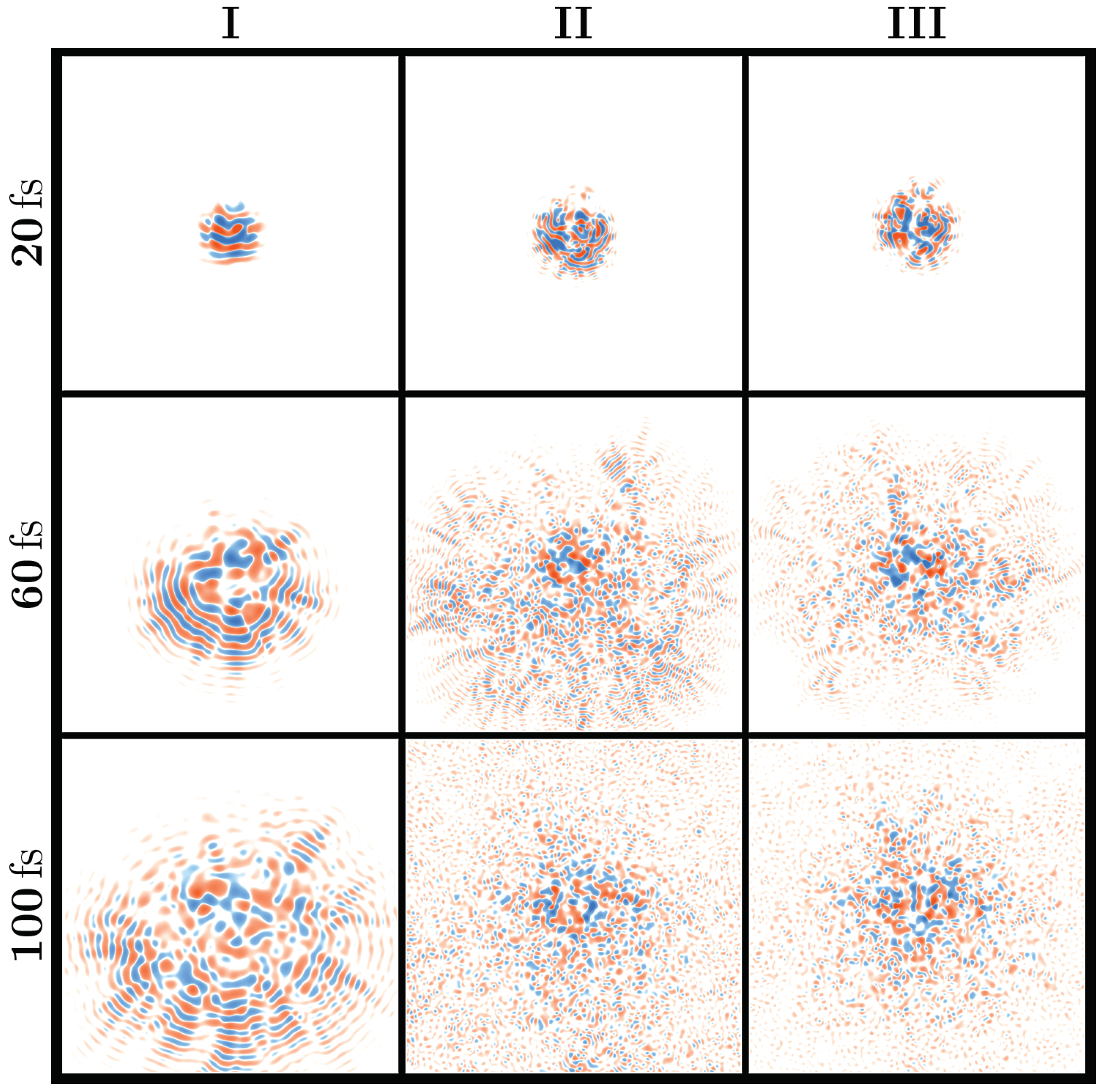
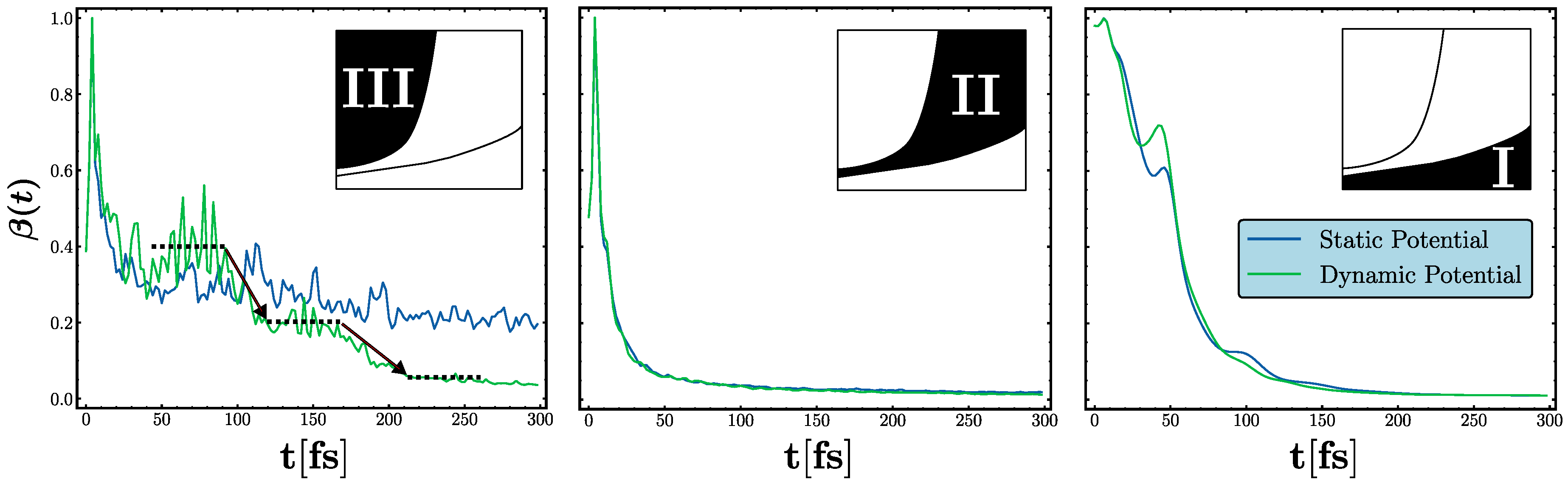
3.2. Transient Localization
4. Conclusion and Future Directions
Author Contributions
Funding
Institutional Review Board Statement
Data Availability Statement
Acknowledgments
Conflicts of Interest
Appendix A. Clustering Analysis
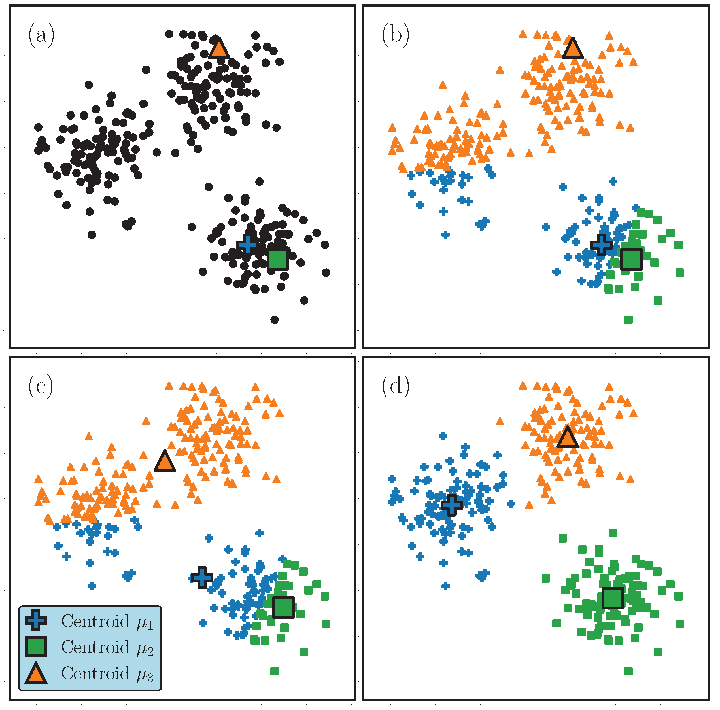
Appendix A.1. k-Means
- Assignment Step: Assign all to their closest centroid, as measured by the squared Euclidean distance. This defines the cluster memberships .
- Update Step: Update the centroids using according to Equation (A2).
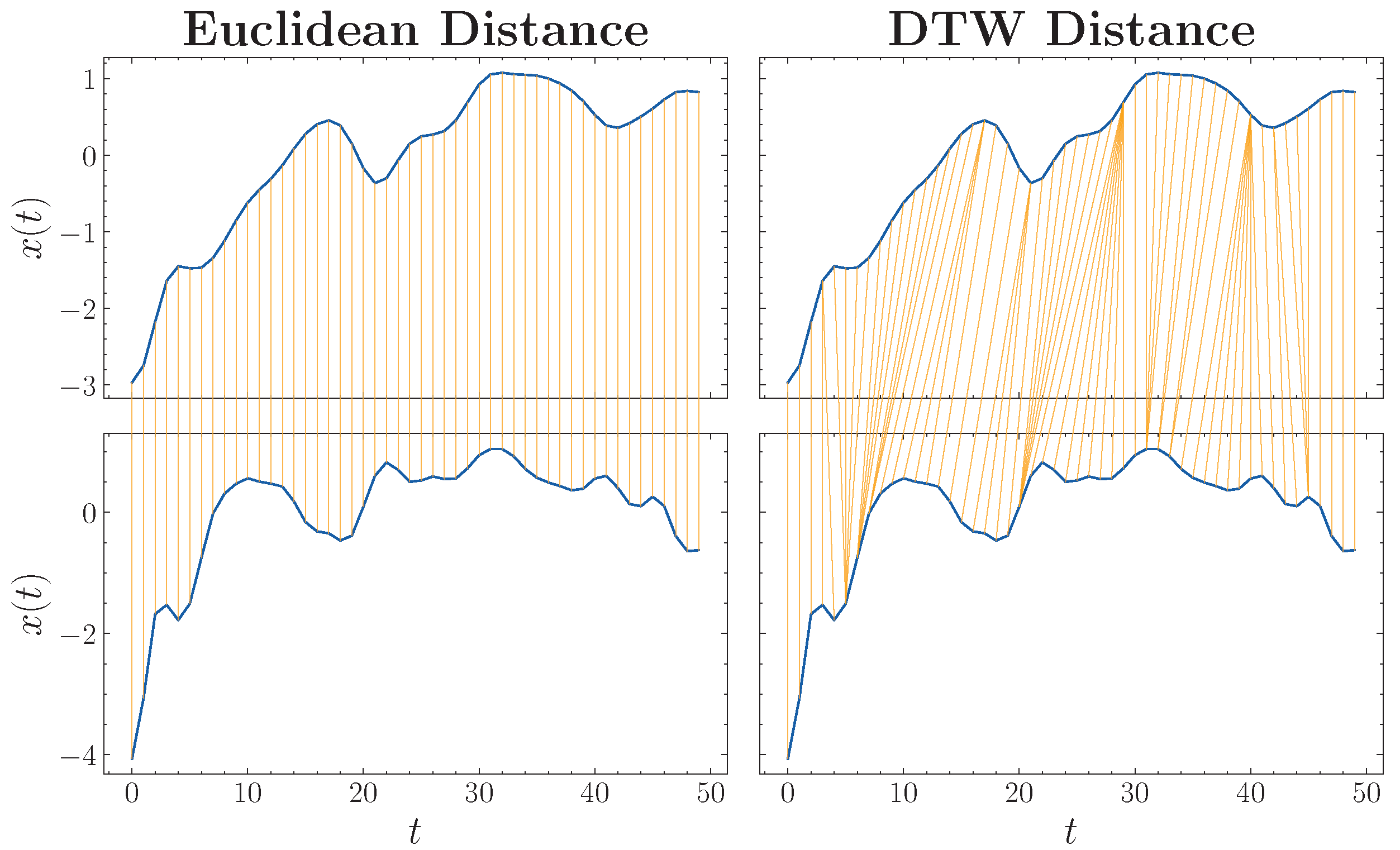
Appendix A.2. Dynamic Time Warping
Appendix A.3. Feature Scaling
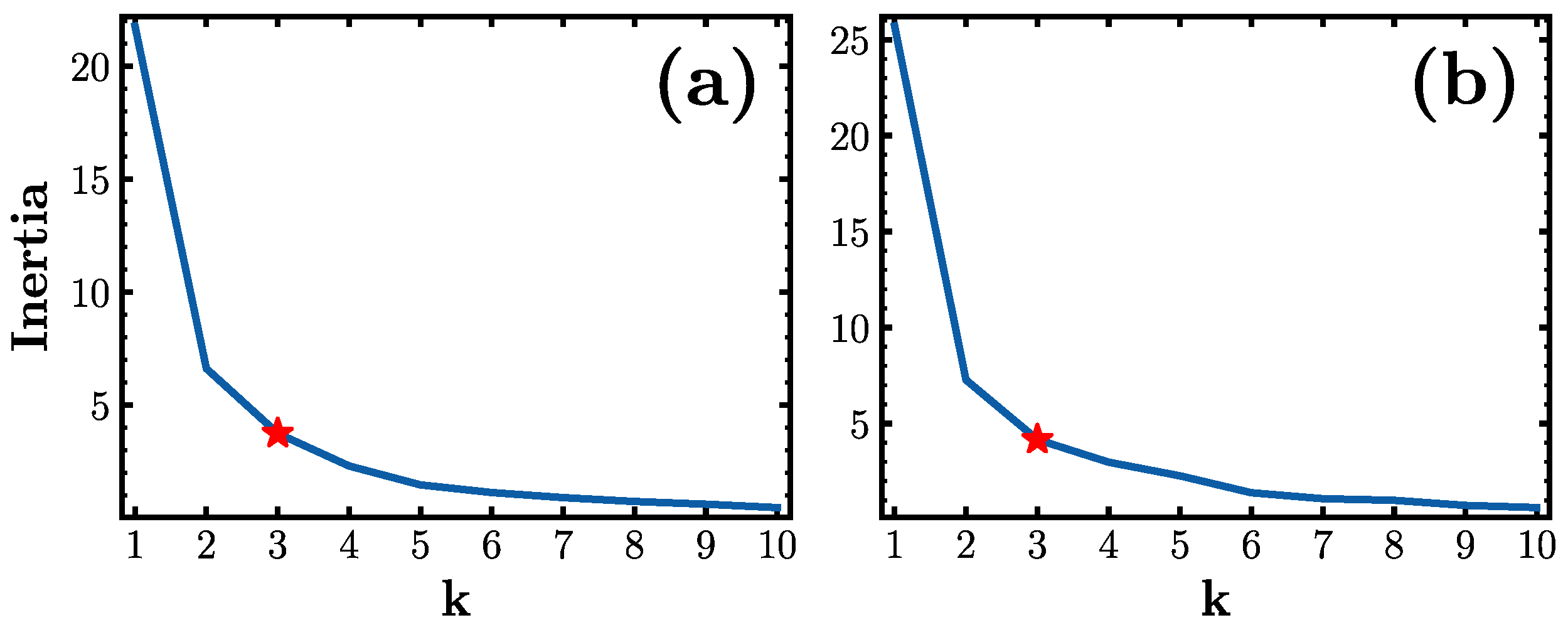
Appendix A.4. Choosing k
Appendix A.5. Ensemble Averaging
Appendix B. Clustering in the Frozen Approximation
References
- Abrahams, E. 50 Years of Anderson Localization; World Scientific: Singapore, 2010; Volume 24. [Google Scholar] [CrossRef]
- Thouless, D.J. Maximum Metallic Resistance in Thin Wires. Phys. Rev. Lett. 1977, 39, 1167–1169. [Google Scholar] [CrossRef]
- Abrahams, E.; Anderson, P.W.; Licciardello, D.C.; Ramakrishnan, T.V. Scaling Theory of Localization: Absence of Quantum Diffusion in Two Dimensions. Phys. Rev. Lett. 1979, 42, 673–676. [Google Scholar] [CrossRef]
- Tarquini, E.; Biroli, G.; Tarzia, M. Critical properties of the Anderson localization transition and the high-dimensional limit. Phys. Rev. B 2017, 95, 094204. [Google Scholar] [CrossRef]
- Gornyi, I.V.; Mirlin, A.D.; Polyakov, D.G. Interacting Electrons in Disordered Wires: Anderson Localization and Low-T Transport. Phys. Rev. Lett. 2005, 95, 206603. [Google Scholar] [CrossRef] [PubMed]
- Fleishman, L.; Anderson, P.W. Interactions and the Anderson transition. Phys. Rev. B 1980, 21, 2366–2377. [Google Scholar] [CrossRef]
- Fleishman, L.; Licciardello, D.C.; Anderson, P.W. Elementary Excitations in the Fermi Glass. Phys. Rev. Lett. 1978, 40, 1340–1343. [Google Scholar] [CrossRef]
- Sacha, K.; Delande, D. Anderson localization in the time domain. Phys. Rev. A 2016, 94, 023633. [Google Scholar] [CrossRef]
- Di Sante, D.; Fratini, S.; Dobrosavljević, V.; Ciuchi, S. Disorder-Driven Metal-Insulator Transitions in Deformable Lattices. Phys. Rev. Lett. 2017, 118, 036602. [Google Scholar] [CrossRef]
- Gogolin, A.; Mel’Nikov, V.; Rashba, E. Conductivity in a disordered one-dimensional system induced by electron-phonon interaction. Sov. J. Exp. Theor. Phys. 1975, 42, 168. [Google Scholar]
- Rashba, E.; Gogolin, A.; Mel’nikov, V. Organic Conductors and Semiconductors; Lecture Notes in Physics; Springer: Berlin/Heidelberg, Germany, 1977; Volume 65. [Google Scholar]
- Anderson, P.W. Absence of Diffusion in Certain Random Lattices. Phys. Rev. 1958, 109, 1492–1505. [Google Scholar] [CrossRef]
- Fratini, S.; Mayou, D.; Ciuchi, S. The transient localization scenario for charge transport in crystalline organic materials. Adv. Funct. Mater. 2016, 26, 2292–2315. [Google Scholar] [CrossRef]
- Troisi, A.; Orlandi, G. Charge-Transport Regime of Crystalline Organic Semiconductors: Diffusion Limited by Thermal Off-Diagonal Electronic Disorder. Phys. Rev. Lett. 2006, 96, 086601. [Google Scholar] [CrossRef]
- Lacroix, A.; de Laissardière, G.T.; Quémerais, P.; Julien, J.P.; Mayou, D. Modeling of Electronic Mobilities in Halide Perovskites: Adiabatic Quantum Localization Scenario. Phys. Rev. Lett. 2020, 124, 196601. [Google Scholar] [CrossRef]
- Kim, D.; Aydin, A.; Daza, A.; Avanaki, K.N.; Keski-Rahkonen, J.; Heller, E.J. Coherent charge carrier dynamics in the presence of thermal lattice vibrations. Phys. Rev. B 2022, 106, 054311. [Google Scholar] [CrossRef]
- Walls, D.; Milburn, G. Quantum Optics; Springer: Berlin/Heidelberg, Germany, 2007. [Google Scholar] [CrossRef]
- Scully, M.; Zubairy, M. Quantum Optics; Cambridge University Press: Cambridge, UK, 1997. [Google Scholar] [CrossRef]
- Grynberg, G.; Aspect, A.; Fabre, C.; Cohen-Tannoudji, C. Introduction to Quantum Optics: From the Semi-Classical Approach to Quantized Light; Cambridge University Press: Cambridge, UK, 2010. [Google Scholar]
- Gerry, C.; Knight, P.; Knight, P. Introductory Quantum Optics; Cambridge University Press: Cambridge, UK, 2005. [Google Scholar]
- Glauber, R.J. Coherent and Incoherent States of the Radiation Field. Phys. Rev. 1963, 131, 2766–2788. [Google Scholar] [CrossRef]
- Shockley, W.; Bardeen, J. Energy Bands and Mobilities in Monatomic Semiconductors. Phys. Rev. 1950, 77, 407–408. [Google Scholar] [CrossRef]
- Bardeen, J.; Shockley, W. Deformation Potentials and Mobilities in Non-Polar Crystals. Phys. Rev. 1950, 80, 72–80. [Google Scholar] [CrossRef]
- Aydin, A.; Keski-Rahkonen, J.; Heller, E.J. Quantum acoustics spawns Planckian resistivity. arXiv 2023, arXiv:2303.06077. [Google Scholar]
- Keski-Rahkonen, J.; Ouyang, X.; Yuan, S.; Graf, A.M.; Aydin, A.; Heller, E.J. Quantum-Acoustical Drude Peak Shift. Phys. Rev. Lett. 2024, 132, 186303. [Google Scholar] [CrossRef] [PubMed]
- Bishop, C.M. Pattern Recognition and Machine Learning; Springer: New York, NY, USA, 2006. [Google Scholar] [CrossRef]
- James, G.; Witten, D.; Hastie, T.; Tibshirani, R. An Introduction to Statistical Learning; Springer: New York, NY, USA, 2013; Volume 112. [Google Scholar] [CrossRef]
- Carleo, G.; Cirac, I.; Cranmer, K.; Daudet, L.; Schuld, M.; Tishby, N.; Vogt-Maranto, L.; Zdeborová, L. Machine learning and the physical sciences. Rev. Mod. Phys. 2019, 91, 045002. [Google Scholar] [CrossRef]
- Zhang, W.; Wang, L.; Wang, Z. Interpretable machine learning study of the many-body localization transition in disordered quantum Ising spin chains. Phys. Rev. B 2019, 99, 054208. [Google Scholar] [CrossRef]
- Van Nieuwenburg, E.P.; Liu, Y.H.; Huber, S.D. Learning phase transitions by confusion. Nat. Phys. 2017, 13, 435–439. [Google Scholar] [CrossRef]
- Carrasquilla, J.; Melko, R.G. Machine learning phases of matter. Nat. Phys. 2017, 13, 431–434. [Google Scholar] [CrossRef]
- Castro, G.A.D.; Gutiérrez, R.P. Artificial neural network for the single-particle localization problem in quasiperiodic one-dimensional lattices. Rev. Mex. Física 2023, 69, 020502-1. [Google Scholar] [CrossRef]
- Wang, L. Discovering phase transitions with unsupervised learning. Phys. Rev. B 2016, 94, 195105. [Google Scholar] [CrossRef]
- Heller, E.J.; Kim, D. Schrödinger Correspondence Applied to Crystals. J. Phys. Chem. A 2019, 123, 4379–4388. [Google Scholar] [CrossRef] [PubMed]
- Kim, D.; Heller, E.J. Bragg Scattering from a Random Potential. Phys. Rev. Lett. 2022, 128, 200402. [Google Scholar] [CrossRef] [PubMed]
- Berry, M.V. Regular and irregular semiclassical wavefunctions. J. Phys. A 1977, 10, 2083. [Google Scholar] [CrossRef]
- Brown, R.H.; Twiss, R.Q. Interferometry of the Intensity Fluctuations in Light. I. Basic Theory: The Correlation between Photons in Coherent Beams of Radiation. Proc. R. Soc. A 1957, 242, 300–324. [Google Scholar] [CrossRef]
- Heller, E.J. The Semiclassical Way to Dynamics and Spectroscopy; Princeton University Press: Princeton, NJ, USA, 2018. [Google Scholar] [CrossRef]
- Tannor, D. Introduction to Quantum Mechanics; University Science Books: Sausalito, CA, USA, 2007. [Google Scholar]
- Keski-Rahkonen, J.; Ruhanen, A.; Heller, E.; Räsänen, E. Quantum Lissajous scars. Phys. Rev. Lett. 2019, 123, 214101. [Google Scholar] [CrossRef]
- Keski-Rahkonen, J.; Luukko, P.J.J.; Kaplan, L.; Heller, E.J.; Räsänen, E. Controllable quantum scars in semiconductor quantum dots. Phys. Rev. B 2017, 96, 094204. [Google Scholar] [CrossRef]
- Keski-Rahkonen, J.; Graf, A.; Heller, E. Antiscarring in Chaotic Quantum Wells. arXiv 2024, arXiv:2403.18081. [Google Scholar]
- Heller, E.J.; Fleischmann, R.; Kramer, T. Branched flow. Phys. Today 2021, 74, 44–51. [Google Scholar] [CrossRef]
- Daza, A.; Heller, E.J.; Graf, A.M.; Räsänen, E. Propagation of waves in high Brillouin zones: Chaotic branched flow and stable superwires. Proc. Natl. Acad. Sci. USA 2021, 118, e2110285118. [Google Scholar] [CrossRef]
- Graf, A.M.; Lin, K.; Kim, M.; Keski-Rahkonen, J.; Daza, A.; Heller, E.J. Chaos-Assisted Dynamical Tunneling in Flat Band Superwires. Entropy 2024, 26, 492. [Google Scholar] [CrossRef]
- Bandrauk, A.D.; Shen, H. Higher order exponential split operator method for solving time-dependent Schrödinger equations. Can. J. Chem. 1992, 70, 555–559. [Google Scholar] [CrossRef]
- Feit, M.; Fleck, J.; Steiger, A. Solution of the Schrödinger equation by a spectral method. J. Comput. Phys 1982, 47, 412–433. [Google Scholar] [CrossRef]
- Kim, D.; Halperin, B.I. Low-energy tail of the spectral density for a particle interacting with a quantum phonon bath. Phys. Rev. B 2023, 107, 224311. [Google Scholar] [CrossRef]
- Thouless, D. Electrons in disordered systems and the theory of localization. Phys. Rep. 1974, 13, 93–142. [Google Scholar] [CrossRef]
- Lloyd, S. Least squares quantization in PCM. IEEE Trans. Inf. Theory 1982, 28, 129–137. [Google Scholar] [CrossRef]
- Sakoe, H.; Chiba, S. Dynamic programming algorithm optimization for spoken word recognition. IEEE Trans. Acoust. Speech Signal Process. 1978, 26, 43–49. [Google Scholar] [CrossRef]
- Varma, C.M. Colloquium: Linear in temperature resistivity and associated mysteries including high temperature superconductivity. Rev. Mod. Phys. 2020, 92, 031001. [Google Scholar] [CrossRef]
- Bednorz, J.G.; Müller, K.A. Possible high Tc superconductivity in the Ba–La–Cu–O system. Z. Phys. B Condens. Matter 1986, 64, 189–193. [Google Scholar] [CrossRef]
- Radaelli, P.; Hinks, D.; Mitchell, A.; Hunter, B.; Wagner, J.; Dabrowski, B.; Vandervoort, K.; Viswanathan, H.; Jorgensen, J. Structural and superconducting properties of La2−xSrxCuO4 as a function of Sr content. Phys. Rev. B 1994, 49, 4163. [Google Scholar] [CrossRef] [PubMed]
- Padilla, W.J.; Lee, Y.S.; Dumm, M.; Blumberg, G.; Ono, S.; Segawa, K.; Komiya, S.; Ando, Y.; Basov, D.N. Constant effective mass across the phase diagram of high-Tc cuprates. Phys. Rev. B 2005, 72, 060511. [Google Scholar] [CrossRef]
- Walsh, C.; Charlebois, M.; Sémon, P.; Sordi, G.; Tremblay, A.M.S. Prediction of anomalies in the velocity of sound for the pseudogap of hole-doped cuprates. Phys. Rev. B 2022, 106, 235134. [Google Scholar] [CrossRef]
- Bozovic, I.; Logvenov, G.; Belca, I.; Narimbetov, B.; Sveklo, I. Epitaxial Strain and Superconductivity in La2−xSrxCuO4 Thin Films. Phys. Rev. Lett. 2002, 89, 107001. [Google Scholar] [CrossRef] [PubMed]
- Legros, A.; Benhabib, S.; Tabis, W.; Laliberté, F.; Dion, M.; Lizaire, M.; Vignolle, B.; Vignolles, D.; Raffy, H.; Li, Z.; et al. Universal T-linear resistivity and Planckian dissipation in overdoped cuprates. Nat. Phys. 2019, 15, 142–147. [Google Scholar] [CrossRef]
- Fang, Y.; Grissonnanche, G.; Legros, A.; Verret, S.; Laliberté, F.; Collignon, C.; Ataei, A.; Dion, M.; Zhou, J.; Graf, D.; et al. Fermi surface transformation at the pseudogap critical point of a cuprate superconductor. Nat. Phys. 2022, 18, 558–564. [Google Scholar] [CrossRef]
- Topinka, M.; LeRoy, B.J.; Westervelt, R.; Shaw, S.; Fleischmann, R.; Heller, E.; Maranowski, K.; Gossard, A. Coherent branched flow in a two-dimensional electron gas. Nature 2001, 410, 183–186. [Google Scholar] [CrossRef]
- Tavenard, R.; Faouzi, J.; Vandewiele, G.; Divo, F.; Androz, G.; Holtz, C.; Payne, M.; Yurchak, R.; Rußwurm, M.; Kolar, K.; et al. Tslearn, A Machine Learning Toolkit for Time Series Data. J. Mach. Learn. Res. 2020, 21, 1–6. [Google Scholar]
- Arthur, D.; Vassilvitskii, S. k-means++: The advantages of careful seeding. In Proceedings of the the Eighteenth Annual ACM-SIAM Symposium on Discrete Algorithms, SODA ’07, New Orleans, LA, USA, 7–9 January 2007; pp. 1027–1035. [Google Scholar]
- Berndt, D.J.; Clifford, J. Using dynamic time warping to find patterns in time series. In Proceedings of the 3rd International Conference on Knowledge Discovery And Data Mining, Seattle, WA, USA, 31 July–1 August 1994; pp. 359–370. [Google Scholar]
- Müller, M. Dynamic Time Warping. In Information Retrieval for Music and Motion; Springer: Berlin/Heidelberg, Germany, 2007; pp. 69–84. [Google Scholar] [CrossRef]
- Brüning, F.; Driemel, A.; Ergür, A.; Röglin, H. On the number of iterations of the DBA algorithm. In Proceedings of the 2024 SIAM International Conference on Data Mining (SDM), Houston, HI, USA, 18–20 April 2024; SIAM: Philadelphia, PA, USA, 2024; pp. 172–180. [Google Scholar] [CrossRef]
- Petitjean, F.; Ketterlin, A.; Gançarski, P. A global averaging method for dynamic time warping, with applications to clustering. Pattern Recognit. 2011, 44, 678–693. [Google Scholar] [CrossRef]

| Parameter | n | a | ||||||
| [Å] | ||||||||
| LSCO | 7.8 | 9.8 | 6000 | 20 | 3.6 | 0.12 | 3.8 | 379 |
Disclaimer/Publisher’s Note: The statements, opinions and data contained in all publications are solely those of the individual author(s) and contributor(s) and not of MDPI and/or the editor(s). MDPI and/or the editor(s) disclaim responsibility for any injury to people or property resulting from any ideas, methods, instructions or products referred to in the content. |
© 2024 by the authors. Licensee MDPI, Basel, Switzerland. This article is an open access article distributed under the terms and conditions of the Creative Commons Attribution (CC BY) license (https://creativecommons.org/licenses/by/4.0/).
Share and Cite
Zimmermann, Y.; Keski-Rahkonen, J.; Graf, A.M.; Heller, E.J. Rise and Fall of Anderson Localization by Lattice Vibrations: A Time-Dependent Machine Learning Approach. Entropy 2024, 26, 552. https://doi.org/10.3390/e26070552
Zimmermann Y, Keski-Rahkonen J, Graf AM, Heller EJ. Rise and Fall of Anderson Localization by Lattice Vibrations: A Time-Dependent Machine Learning Approach. Entropy. 2024; 26(7):552. https://doi.org/10.3390/e26070552
Chicago/Turabian StyleZimmermann, Yoel, Joonas Keski-Rahkonen, Anton M. Graf, and Eric J. Heller. 2024. "Rise and Fall of Anderson Localization by Lattice Vibrations: A Time-Dependent Machine Learning Approach" Entropy 26, no. 7: 552. https://doi.org/10.3390/e26070552
APA StyleZimmermann, Y., Keski-Rahkonen, J., Graf, A. M., & Heller, E. J. (2024). Rise and Fall of Anderson Localization by Lattice Vibrations: A Time-Dependent Machine Learning Approach. Entropy, 26(7), 552. https://doi.org/10.3390/e26070552