Abstract
To meet the challenges of energy sustainability, the integrated energy system (IES) has become a key component in promoting the development of innovative energy systems. Accurate and reliable multivariate load prediction is a prerequisite for IES optimal scheduling and steady running, but the uncertainty of load fluctuation and many influencing factors increase the difficulty of forecasting. Therefore, this article puts forward a multi-energy load prediction approach of the IES, which combines the fennec fox optimization algorithm (FFA) and hybrid kernel extreme learning machine. Firstly, the comprehensive weight method is used to combine the entropy weight method and Pearson correlation coefficient, fully considering the information content and correlation, selecting the key factors affecting the prediction, and ensuring that the input features can effectively modify the prediction results. Secondly, the coupling relationship between the multi-energy load is learned and predicted using the hybrid kernel extreme learning machine. At the same time, the FFA is used for parameter optimization, which reduces the randomness of parameter setting. Finally, the approach is utilized for the measured data at Arizona State University to verify its effectiveness in multi-energy load forecasting. The results indicate that the mean absolute error (MAE) of the proposed method is 0.0959, 0.3103 and 0.0443, respectively. The root mean square error (RMSE) is 0.1378, 0.3848 and 0.0578, respectively. The weighted mean absolute percentage error (WMAPE) is only 1.915%. Compared to other models, this model has a higher accuracy, with the maximum reductions on MAE, RMSE and WMAPE of 0.3833, 0.491 and 2.8138%, respectively.
1. Introduction
Energy is a key factor in promoting economic growth, providing the foundation for the development of human society, and plays an extremely important role in human society [1]. However, fossil energy sources are facing a growing shortage. At the same time, the problems of inefficiency, energy waste and environmental pollution of traditional thermal power generation are becoming more and more prominent. Therefore, there is an urgent need for the energy system to accelerate its transformation [2]. Traditional energy system construction has largely been an extension in depth within single systems. There is minimal physical interconnection and information interaction between these systems, which hinders the complementary and mutually advantageous use of diverse energy sources. In order to cope with these shortcomings and promote the development of renewable energy sources, the integrated energy system is born at the right moment [3,4].
The IES reduces the use of conventional energy sources and increases the proportion of renewable energy sources to meet the targets of carbon peaking and carbon neutrality [5]. It has an efficient and flexible energy supply mode, coupling various modalities of energy, for instance, electricity, cooling and heating loads. Through the interconnection and optimized scheduling of energy, the efficient use and sustainable development of energy in the whole system are greatly realized [6]. In this intelligent energy system, accurate short-term forecasting of the user-side multi-energy load is extremely important for maintaining the balance between energy supply and demand, optimizing energy dispatch, and ensuring the safe and stable operation of the system [7]. This need has prompted it to become a significant area in current academic research.
It has an important practical value to carry on an accurate multi-energy load prediction. In recent years, many scholars have focused on tackling the issues of accuracy and reliability in IES multi-energy load prediction, proposing numerous load predictive methodologies. As a result, the field has seen a gradual enrichment of research outcomes. Current load forecasting methods mainly include two categories [8,9,10]. The former are traditional linear prediction methods, such as the exponential smoothing method [11], linear regression method [12], time series method [13], Kalman filter algorithm [14], etc. Such methods often fail to effectively explore the inherent characteristics of power load data, and it is difficult to achieve the increasing accuracy of load prediction. The latter are advanced machine learning ways, for instance, fuzzy theory [15], support vector machine [16], artificial neural network [17,18,19], deep neural network [20,21,22,23], etc. These methods are highly capable and adaptive to learn the intrinsic correlation between data efficiently and have been widely used in the domain of IES multi-energy load prediction. In reference [24], the convolutional neural network (CNN) is first applied to fetch hidden features, and the features are taken as inputs. A bidirectional gated recurrent unit (BIGRU) network is used to forecast IES electricity, cooling and heating loads, and three attention mechanism modules are combined to enhance the impact generated by the important information. In reference [25], a multi-task learning architecture with homoscedasticity uncertainty and a multiple load prediction model integrating multiple gated cyclic unit neural network (GRU) strategies was constructed, which could realize the sharing of different network results according to the volatility degree in different loads. Nevertheless, the forecasting accuracy is not high due to the failure to consider weather and other related factors. Meteorological factors, as important input features for load forecasting, to some extent affect users’ energy demand, which in turn affects load power. In reference [26], correlation analysis between multiple loads and between multiple loads and meteorological elements is carried out and then a long short-term memory network (LSTM) is applied to subsequent forecasting work. However, deep neural networks increase the complexity and difficulty of the training process. There are many hyperparameters to be tuned [27], which leads to a high training time and computational cost when processing large-scale data, and takes a long time to converge and achieve the best performance. The extreme learning machine (ELM) is trained in the manner of random initialization without complex iterative optimization process, and the training speed is very fast [28,29]. Moreover, there is no need to adjust a quantity of hyperparameters, simplifying the design and realization for the model. The kernel extreme learning machine is an improvement based on ELM, which introduces kernel function mapping to replace the random mapping relationship between the input and output of the hidden layer. While retaining the good predictive performance of ELM, it avoids the problem of large randomness in training results caused by manually setting the number of nodes, and has better robustness [30]. However, a single kernel function has the disadvantage that it is hard to completely adjust to various data features. In references [31,32,33], a hybrid kernel extreme learning machine (HKELM) was obtained by combining the advantages of different kernel functions and weighting. It has the performance of efficiently dealing with intricate nonlinear characteristics, and can readily strengthen the final forecasting effect. However, the HKELM model is highly sensitive to the selection of kernel parameters and penalty coefficients [34,35,36]. The difficulty of visually identifying the best parameter combinations may lead to a loss of accuracy in the prediction results.
Aiming at the problems of numerous meteorological factors that affect load forecasting and the strong randomness of manually selecting HKELM kernel parameters and penalty coefficients, this paper proposes an IES multi-energy load forecasting method using the FFA-HKELM model. Firstly, the comprehensive weight method integrates the entropy weight method with Pearson correlation coefficients to evaluate the relevance and information content of the features concurrently. This approach reduces the dependence on a single feature selection criterion. The influential factors that are highly related to the three types of loads are selected as model features and input into the HKELM weighted by two kernel functions for training. Then, the key parameters for the model are optimized employing a novel FFA method to obtain the FFA-HKELM model with optimal parameter combinations. Eventually, the model is adopted in the actual integrated energy system of the Tempe area in the United States, and the electrical, heating and cooling loads are forecast in the short term. Comparing the results with other forecasting methods, it is verified that this method can better realize the accurate prediction of future multiple load values through the analysis of multiple evaluation indexes.
This article is arranged as follows. Section 2 describes the theory of the combined weights approach and the analysis of the relevant factors in the IES. Section 3 introduces the FFA algorithm, HKELM and the process of establishing the FFA-HKELM prediction model. Meanwhile, the optimization effect of the FFA algorithm is compared with other algorithms. Section 4 analyzes the predictive performance of this model and other comparative models. Section 5 is the summary of this paper and the future research plan.
2. Analysis of IES Structure and Feature Variable Screening
2.1. IES Structure
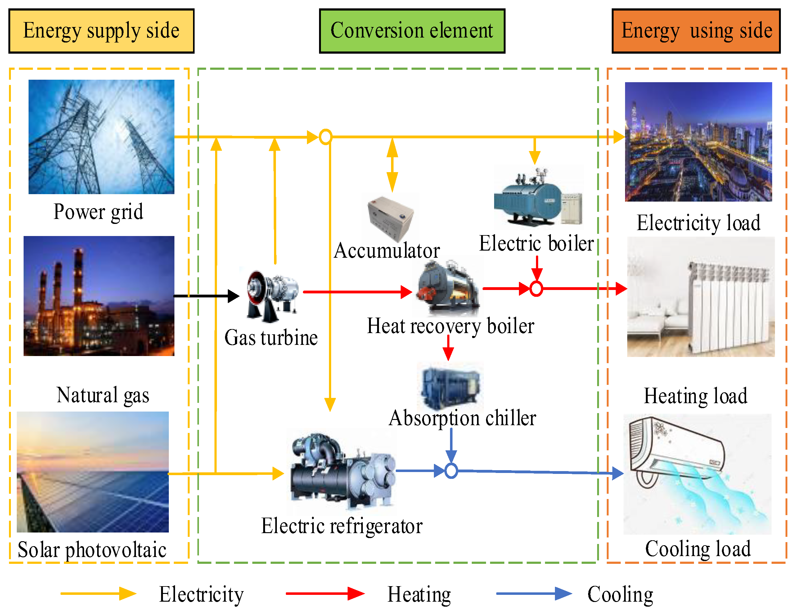
IES, as a new type of energy system, optimizes the whole process of energy production, transmission, storage and use. It can efficiently harness renewable energy sources, ensuring their optimal use. Additionally, it achieves gradient utilization of non-renewable energy sources, promoting the synergistic operation of various energy types. This approach enhances the overall energy utilization efficiency [37]. The schematic diagram of the system is shown in Figure 1. The electrical loads are provided by gas turbines, storage batteries, photovoltaic devices and external grids. The cooling load is provided by electric chillers and absorption chillers. The heating load is mainly provided by electric boilers and waste heat boilers.
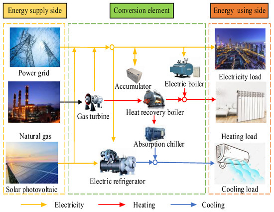
Figure 1.
Schematic diagram of IES structure.
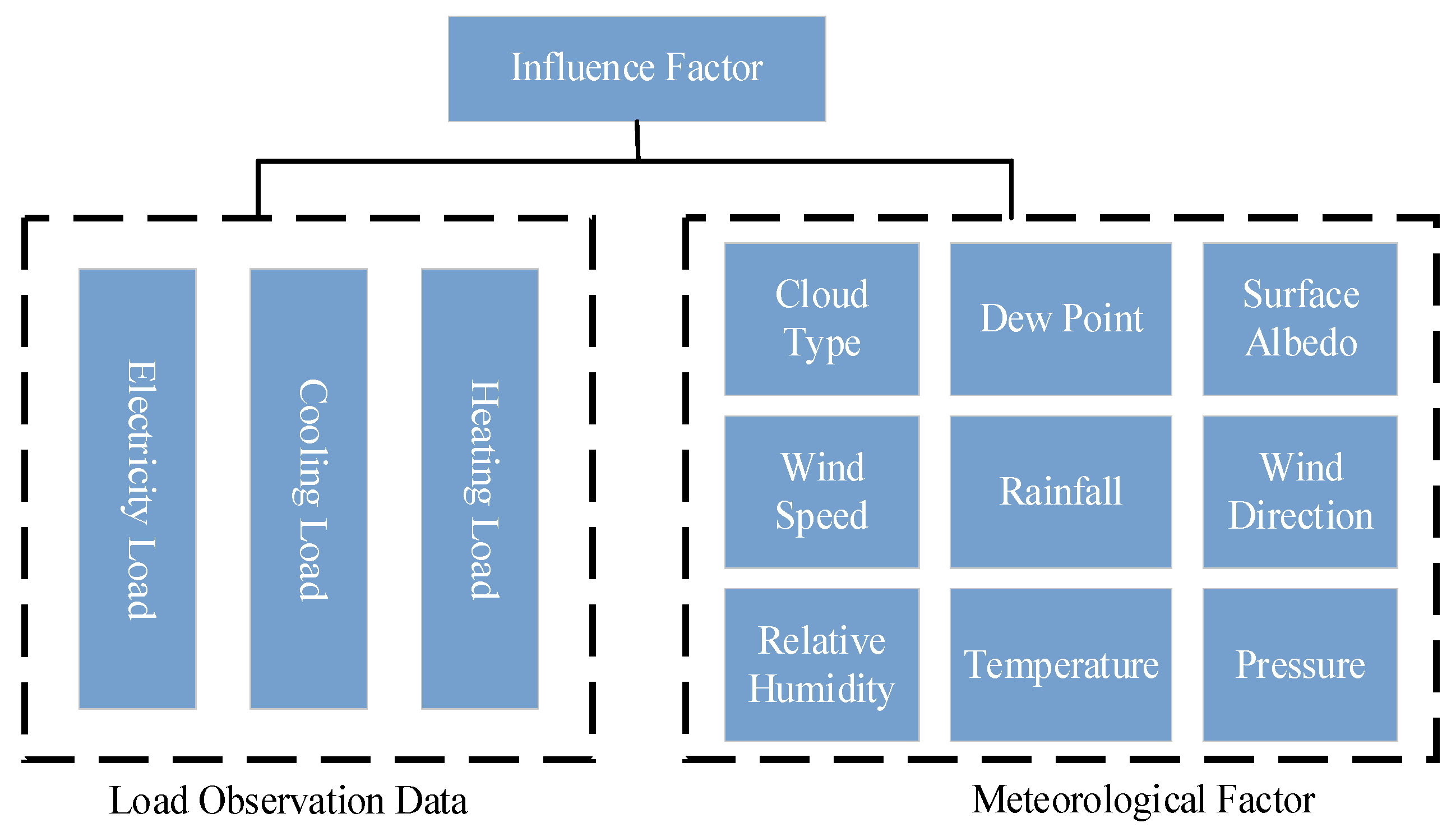
During the energy conversion process, the consumption by various types of loads necessitates the collaborative functioning of multiple energy subsystems. This means that different energy subsystems interact with each other. Therefore, there is a certain degree of close relationship between electrical, heating and cooling loads in the IES. In addition, terminal users have uncertainties when using different loads, which are readily impacted by meteorological elements, for instance, rainfall and temperature. Climate change directly affects user demand for workload. When selecting input characteristics, external meteorological factors should be taken into account, all of which are shown in Figure 2.
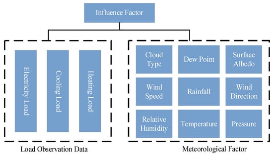
Figure 2.
Multi-energy load influencing factors.
2.2. Entropy Weight Method
Entropy weighting is an objective weighting method, which can fully explore the inherent laws and information of the original data, and the final weights will not be affected by the subjective experience or preference of the decision maker.
In information theory, entropy is a measure of uncertainty, and the degree of randomness and disorder can be determined by calculating the entropy value. A smaller information entropy value for an indicator signifies a higher degree of variability, implying that it offers more information. Consequently, this indicator assumes a more significant role in comprehensive evaluation, which is reflected in its greater weight. On the contrary, the greater the information entropy of an indicator, the lower the variability of the indicator and the less information it provides. Therefore, the smaller the role it can play in the comprehensive evaluation, the lower the corresponding weight. The detailed calculation process is as follows:
- Construct a standardized matrix of indicator data: The index data of the initial data matrix are normalized.
- Computational information entropy: The output entropy of each index is calculated from the normalized standard matrix. The entropy value can be calculated as follows:where represents the information entropy of the index; indicates the number of all indicators; represents the normalized value of the indicator.
- Determine index weight: The information entropy of each index is used to determine its weight. The weight is calculated as follows:where represents the weight of an indicator.
The information weight is a key measure of the information content of an indicator. A high weight means that the indicator has a significant impact on the decision-making outcome. Using the calculation of information entropy and weights, it is possible to set a weight distribution for decision-making tasks. This helps decision makers to make informed decisions among different indicators and enhances the accuracy and reliability of decision making. However, information weighting mainly focuses on the diversity and uncertainty of indicators without fully considering the interactions between them. Therefore, in practical applications, it is essential to fully consider the combined impact of indicators in conjunction with other assessment methods and expertise.
As can be seen from Table 1, the weight value of Cloud Type is as high as 0.423, indicating that the dispersion of data distribution of this indicator is enhanced, and thus contains more abundant information. The weights of Cooling, Heating, Surface Albedo, Relative Humidity, Rain, Wind Speed, Wind Direction, Temperature and Electricity are 0.1017, 0.0746, 0.0740, 0.0740, 0.0684, 0.0528, 0.0401, 0.0313 and 0.0278, respectively. The weights of Dew Point and Pressure are 0.0165 and 0.0158, respectively, indicating a low degree of variability in these two indicators.

Table 1.
The index weight results are obtained by entropy weight method.
2.3. Pearson Correlation Coefficient Method
However, considering the comprehensiveness of the influencing factors and using all elements as potential input features will bring too much noise during the feature selection process for IES multi-energy load forecasting. It leads to some extraneous elements being added to the model, which often brings negative impacts and instead reduces the computational efficiency and prediction accuracy [38]. Therefore, so as to quantitatively analyze the influence level with internal and external factors and efficiently screen out the key influence indexes, this paper adopts the Pearson correlation coefficient to analyze the degree of relevance between electricity, cooling, heating loads and external meteorological factors. Assuming that there are two sample sequences and , the specific expression of this coefficient is as follows:
where is the amount of data for each group of samples. and refer to the mean value of sequences , , severally. The value of ranges from −1 to 1.
The Pearson correlation coefficients between the electrical, heating, cooling loads and the meteorological data of the IES in the Tempe area are obtained by calculations and the consequences of the correlations are presented in Table 2.
Table 2.
Pearson correlation among all factors.
As shown in Table 2, the correlation between electrical and heating loads of the IES in the Tempe area is extremely strong. The strong degree of relevance between heating and cooling loads as well as between heating and electrical loads indicates that any two loads interact with each other. At the same time, there is a strong degree of relevance between electric, heating, cooling loads and dew point, rainfall, temperature and pressure, and a weak correlation with cloud type, surface albedo, wind direction, humidity and wind speed. Among them, the absolute value of the obtained Pearson correlation coefficients for temperature and precipitation, as key indicators directly related to the production and life of the users, is more than 0.55, illustrating that the impact of these two factors on the changes in load is particularly prominent. The positive correlation between pressure and cooling load is high, indicating that pressure positively affects users’ cooling habits.
2.4. Comprehensive Weight Method Analysis of Multi-Energy Load Relevant Factors
The composite weight method is a variable screening technique that incorporates the entropy weight method and the Pearson correlation coefficient. This method is designed to assess and select characteristic variables by integrating the Pearson correlation coefficient with the information weight of each variable. It determines their combined weights through this integrated evaluation, providing a comprehensive measure of their significance. The Pearson correlation coefficient of each characteristic variable is multiplied with its entropy weight to arrive at its composite weight value. The calculation of the composite weights is based on the following formula:
where represents comprehensive weight, represents information weight, and represents the Pearson correlation coefficient. The higher the value of the variable, the more critical the role it plays in predicting the target variable, and the stronger the correlation.
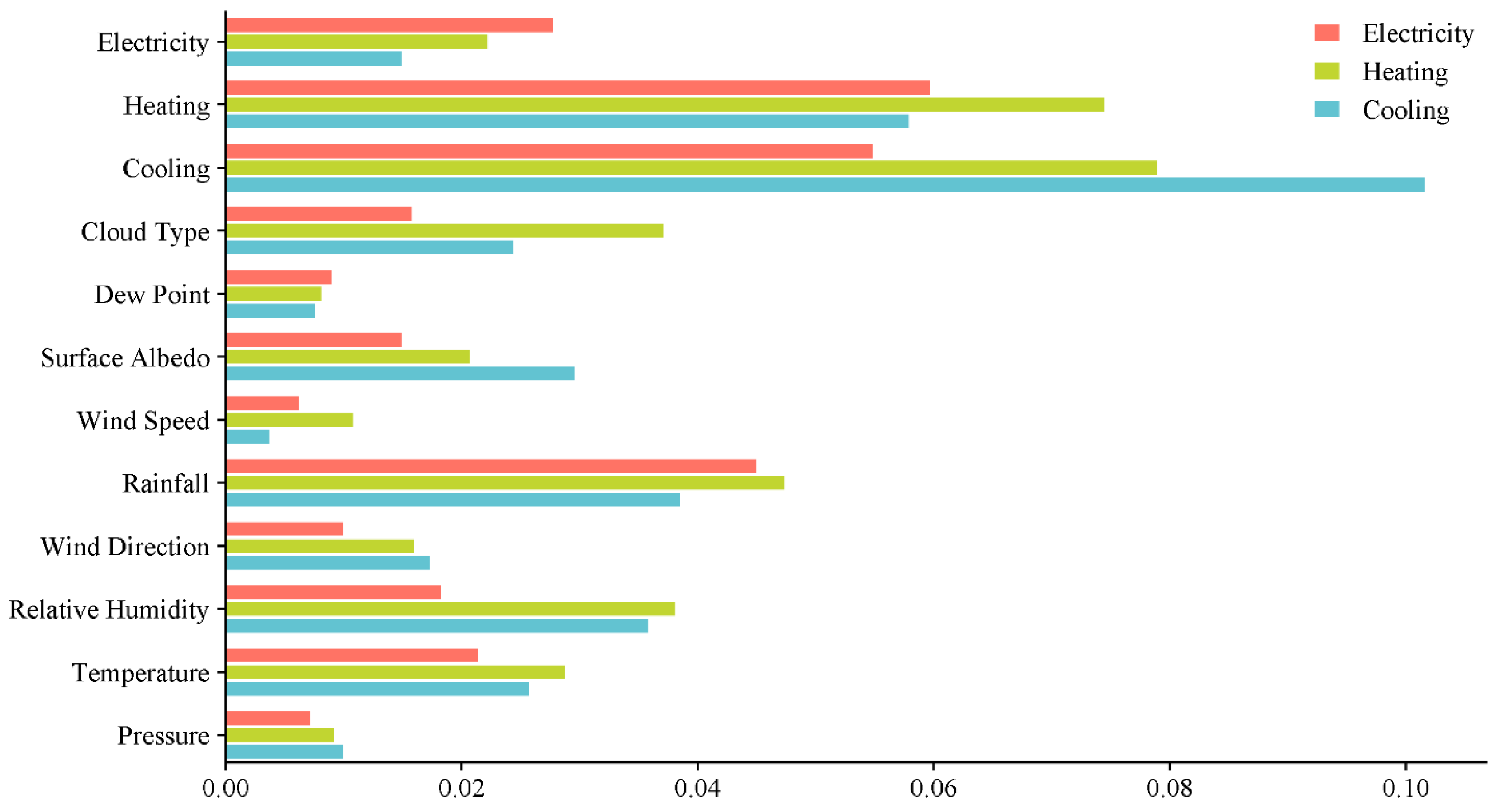
The advantage of the comprehensive weighting method is that it not only covers the consideration of linear relationships, but also includes the analysis of key factors, providing a more comprehensive evaluation and screening framework for characteristic variables. This method enhances the accuracy and reliability of feature selection. Based on the results of the combined weight calculations presented in Table 3 and Figure 3, the following input variables were selected to predict the different target variables:
Table 3.
The comprehensive weight value of each target variable.

Figure 3.
The comprehensive weight of each characteristic variable.
- Electricity prediction: Electricity, Heating, Cooling, Cloud Type, Surface Albedo, Rainfall, Wind Direction, Relative Humidity, Temperature;
- Heating prediction: Electricity, Heating, Cooling, Cloud Type, Surface Albedo, Wind Speed, Rainfall, Wind Direction, Relative Humidity, Temperature;
- Cooling prediction: Electricity, Heating, Cooling, Cloud Type, Surface Albedo, Rainfall, Wind Direction, Relative Humidity, Temperature, Pressure.
These input variables are selected based on their combined weights, taking into account the Pearson correlation coefficient and information weights. The integration of these variables into the forecasting model is expected to increase the accuracy and stability of electrical, heating and cooling loads forecasting.
3. Multi-Energy Load Prediction Model Using FFA-HKELM
3.1. Fennec Fox Optimization Algorithm
The fennec fox optimization algorithm is an innovative heuristic algorithm suggested by Trojovsky [39] in 2022, which simulates the predation behavior of fennec foxes in nature for calculation. Comparing the effects with the conventional optimization algorithm, it can achieve convergence at a faster rate and find a better plan in a shorter time. And in high-dimensional spaces, it can effectively avoid a slide into local optimal solutions. The key strategy for the FFA algorithm is divided into two phases: development and exploration, specifically, the natural behavior of the fennec foxes in digging up the sand in search of prey and avoiding predator attacks.
Firstly, the fennec fox population is randomly initialized according to the boundary of this question, and the concrete procedure is the following:
where refers to the control variable. refers to the number of all fennec foxes. is the quantity of control variables. The interval of random digit is [0, 1]. and refer to the upper and lower boundaries of the control variable, severally.
After initializing the population, the individual position of the population is updated in the search space according to the two stages of the fennec fox’s natural behavior. The specific process is as follows:
The first stage is development. At night, fennec foxes hunt alone, using their large ears to detect potential prey under the sand. Once they find their target, they burrow with their feet, leaving prey exposed for easy capture. This hunting behavior can be regarded as a local search, and simulating this behavior can help to improve the problem-solving ability and thus increase the possibility of obtaining a globally optimal solution. Assume a neighborhood of radius R centered on the actual position of the fennec fox. The fennec fox searches locally in this area to obtain the optimal solution, and its position update formula is shown below.
where refers to the new location of the fennec fox after updating for the development phase. refers to the present iteration amount. is the constant 0.2. refers to the maximum iteration amount. refers to the radius of the neighborhood of .
If the objective function deserves to be improved, then the location of the fennec fox will also change. The concrete procedure is the following:
where refers to the outcome of the objective function in this development phase. refers to the new position of the fennec fox in the first phase.
The second stage is exploration. Fennec foxes may be prey for feral predators, for instance, caracals and hyenas. Despite this, they are able to successfully evade these predators with their incredible speed of movement. This evasion strategy becomes the basis of the global search, and simulating this strategy helps to avert a slide into local optimal solutions. Then, for the second stage, the locations of fennec foxes are updated according to Formulas (8) and (9).
where refers to the location of the fennec fox’s escape target. refers to the fennec fox after the update of the exploration phase. refers to the outcome of the objective function. The interval of the random number is [1,2].
If the objective function value becomes better at this location, the process of updating the location of the fennec fox is the following:
where is the new position of the fennec fox in the second stage. is the value of the objective function in the exploration stage.
3.2. FFA Performance Evaluation
The pseudo-code of the specific implementation steps of the FFA algorithm is in Algorithm 1. So as to investigate the effectiveness of the FFA algorithm, this article compares the optimization results of this algorithm with the grey wolf optimizer algorithm (GWO) [40], whale optimization algorithm (WOA) [41] and sparrow search algorithm (SSA) [42], severally. The download address is https://seyedalimirjalili.com/projects (accessed on 15 January 2024). The quantity of populations and the maximum quantity of iterations for whole algorithms are considered as 30 and 500. The experiments are performed in MATLAB R2021a software using a 64-bit Core i5 processor with 2.50 GHz and 16 GB main memory in Windows 11.
| Algorithm 1 Pseudo-code of the FFA algorithm |
| Start FFA. |
|
|
|
|
|
|
|
|
|
|
|
| End FFA. |
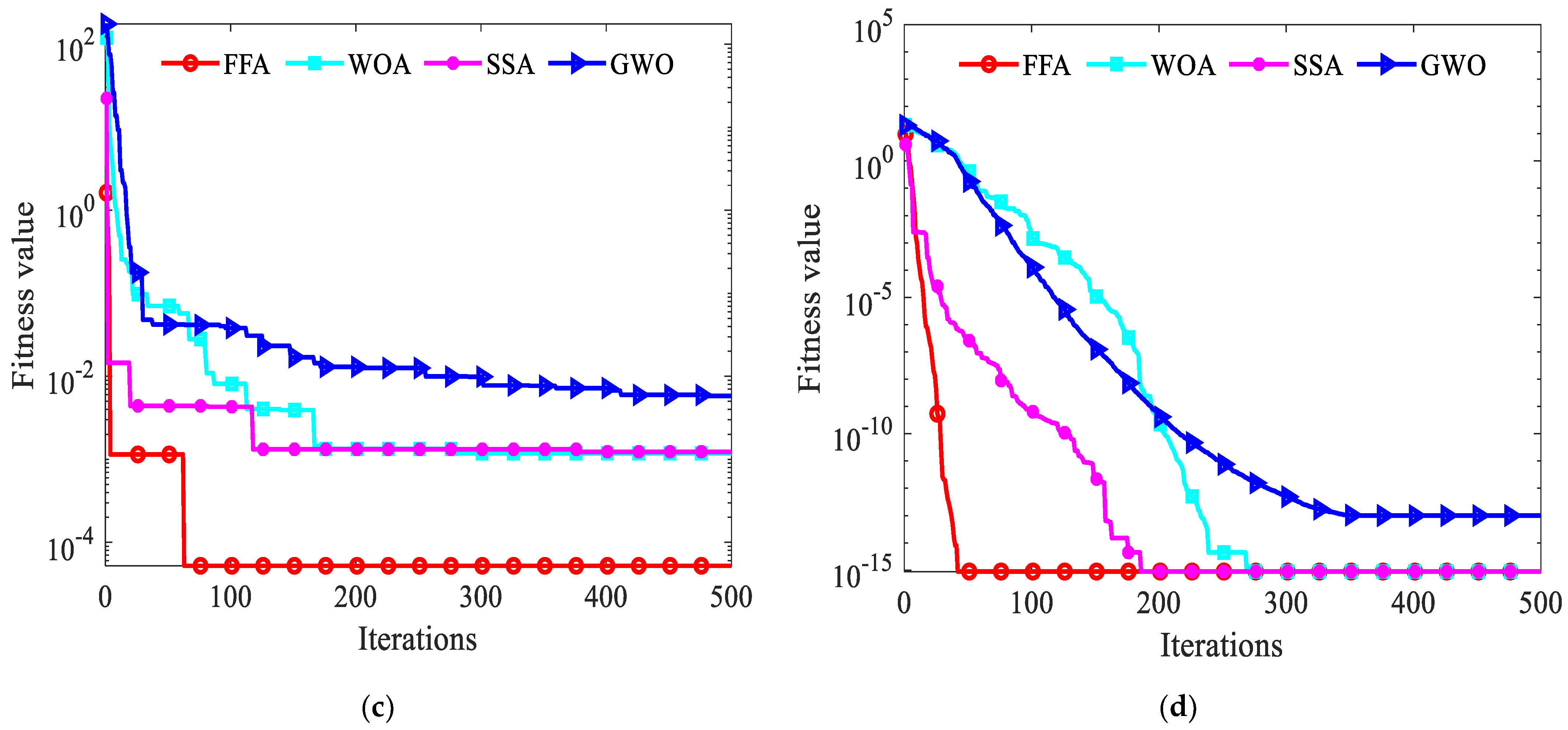
Different benchmarking functions are also selected so as to comprehensively verify the reliability of the optimization algorithms. Four distinct algorithms are independently executed 30 times each. The average of these results is taken as the final outcome. This approach effectively negates the influence of random factors, thereby enhancing the credibility and persuasiveness of the experimental findings. The convergence curves of all algorithms are illustrated in Figure 4.
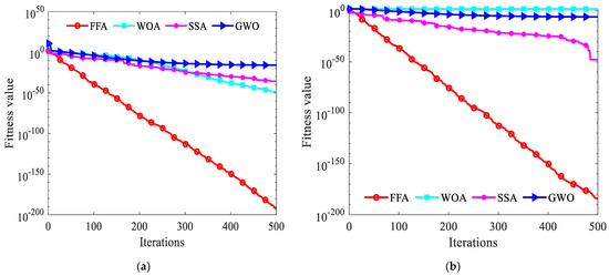
Figure 4.
(a) The first benchmarking function; (b) the second benchmarking function; (c) the third benchmarking function; (d) the fourth benchmarking function.
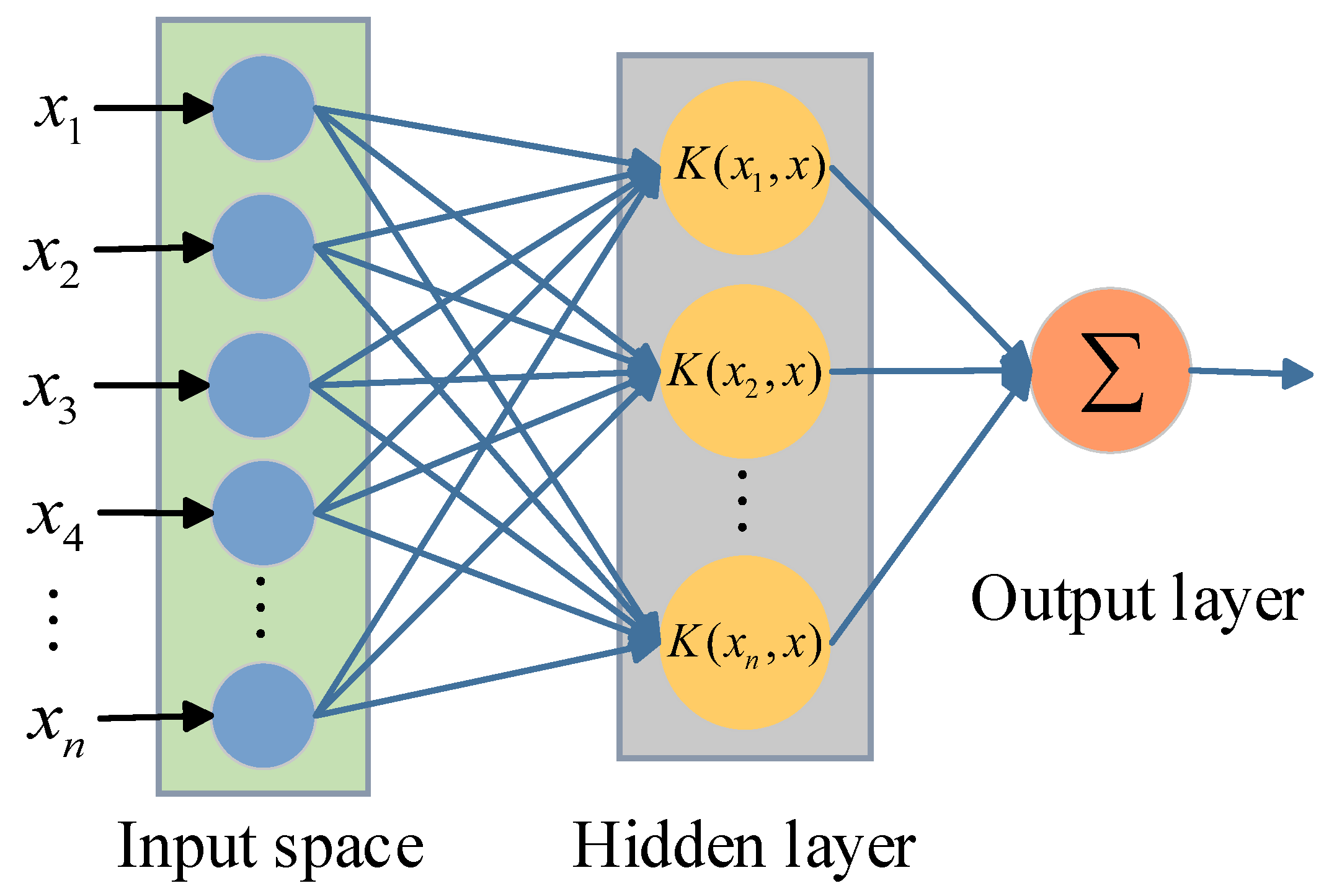
3.3. HKELM Algorithm
ELM is a feedforward neural network based on a single layer that creates weights and thresholds at random. During the training process, a unique and optimal solution can be obtained by adjusting only the number of hidden layer neurons without making any other adjustments. Therefore, ELM has better convergence speed and efficiency. However, when there are multiple unknown datasets in the model, the accuracy of ELM is relatively low. The kernel extreme learning machine (KELM) is an improved algorithm developed by combining ELM and kernel function. It not only fully retains the original advantages of ELM, but also improves the prediction performance and stability of the model. Its network framework is as illustrated in Figure 5, where K is the kernel function matrix.

Figure 5.
KELM network structure diagram.
The expression for the KELM output model is shown below.
where is network output. and are mapping matrices. refers to the penalty coefficient. refers to the aim vector. refers to the unit matrix.
The kernel function in this model can be defined by the following Equation (12).
The input data are transformed into feature vectors in a high-dimensional space by mapping the kernel function, which is thus obtained:
Radial basis kernel function and polynomial kernel function are two common kernel functions; the specific expressions are shown below.
where and are the kernel parameters of the polynomial kernel function, respectively. is the nuclear parameter of the radial basis kernel function.
The selection of appropriate kernel functions has a significant impact on the performance of the KELM model; therefore, finding a suitable kernel function is crucial for the KELM model. So as to comprehensively heighten the generalization and learning ability of KELM, this article combines the radial basis kernel function and polynomial kernel function as the kernel function of the KELM model by linear combination, and combines the benefits of these two kernel functions to obtain a new HKELM model, whose expression is as follows:
where is the weight coefficient of HKELM.
3.4. Establishment of FFA-HKELM Prediction Model
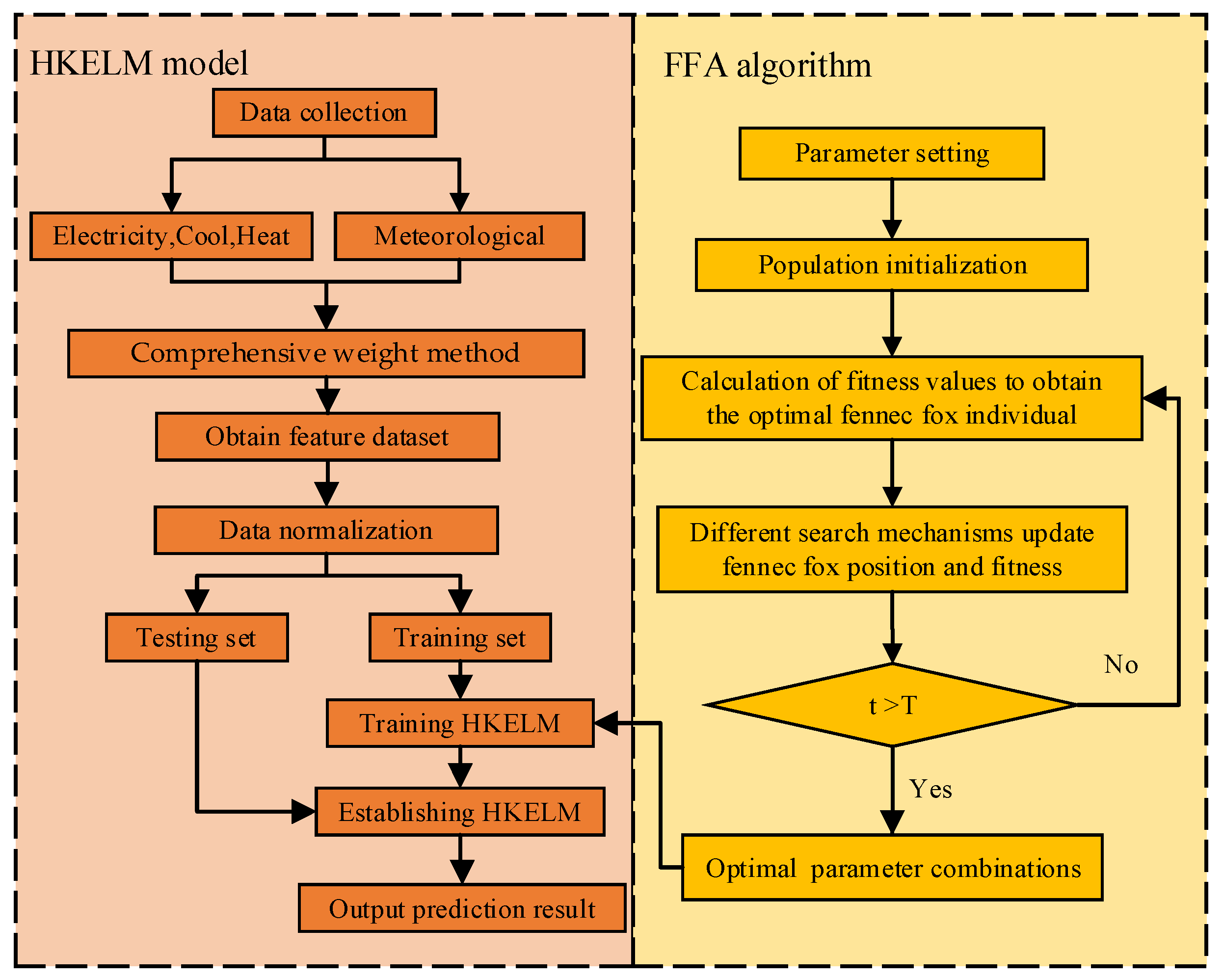
The precision of prediction for the HKELM model is determined by the mixed kernel parameters and penalty parameters , so it is particularly important to optimize these key parameters. Here, the FFA method is used for optimization, and the FFA-HKELM model is established to achieve the prediction of the electric cooling and heating loads. The whole framework procedure is as illustrated in Figure 6, and the specific process is the following.
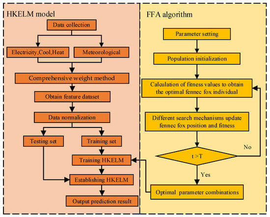
Figure 6.
Frame structure diagram of FFA-HKELM model.
(1) The comprehensive weighting method is applied to combine the entropy weight method and Pearson correlation coefficient, fully considering the correlation and information of each feature, in order to select appropriate input features to build a multivariate time series for IES load forecasting.
(2) The dataset is divided and normalized, and the resulting training set is input into the FFA-HKELM model to seek out the optimal parameter combinations by means of the FFA algorithm.
(3) Set the parameters of the FFA algorithm, namely, population quantity , the quantity of iterations , variable dimension , and upper and lower limits .
(4) Initialize the population by combining all the mixed core parameters and punishment parameters as the position of each fennec fox, and initialize the position of individual fennec foxes by Formula (5).
(5) Calculate and sort the fitness values of individual fennec foxes, find out the lowest fitness value as the optimal fennec fox individual, and the mean square error is considered as the fitness function.
(6) Update the location and fitness of the fennec fox population. The numerical value of fitness for the current iteration optimal fennec fox is in comparison with the value of the last iteration optimal fennec fox. If the result is better than the previous generation, it is updated; otherwise, it is unchanged.
(7) Determine if the quantity of iterations has been reached. In case the quantity is reached, the process ends. Input the optimal mixed kernel parameters and penalty parameters combination into the HKELM model; otherwise, go to Step 5.
(8) The numerical value of the corresponding features in the test set is input into the constructed FFA-HKELM model for the forecasting of electric heating and cooling loads in the IES.
4. Experimental Simulation Analysis
4.1. Experimental Data
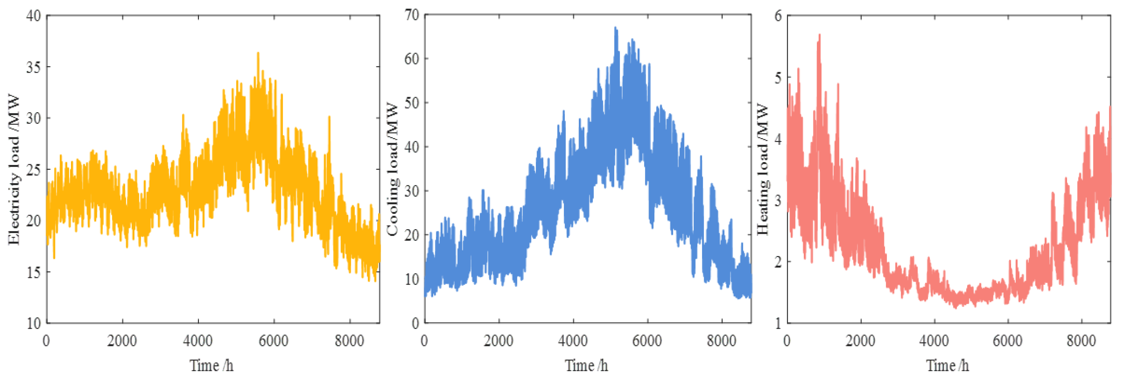
In the article, the measured values of the integrated energy system provided by the Tempe regional network platform of Arizona State University from 1 January to 31 December 2020 are used for the experiment [43]. The sampling period of the data is 1 h and contains a total of 8784 sample points, and the measured numerical values from 1 January to 26 December 2020 are trained to forecast electrical, heating and cooling loads from 27 December to 31 December 2020. The measured electrical, heating and cooling loads are different in dimensions, and these three loads need to be converted into a unified unit MW, where the unit relationship between different loads is 1 MW = 284 Ton = 3.4 MMBtu/h. Figure 7 shows the variations for the processed loads.
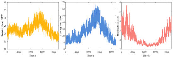
Figure 7.
The electricity, cooling and heating loads change curves.
4.2. Model Performance Evaluation Index
So as to comprehensively and quantitatively measure the predictive performance of the model, this paper adopts three commonly used error evaluating indexes, namely mean absolute error (MAE), root mean square error (RMSE) and mean absolute percentage error (MAPE), through intuitive error analysis. The smaller the error evaluation index value, the smaller the whole error between predicted and observed values, the better the prediction performance of the model. The weighted mean absolute percentage error (WMAPE) is applied to measure the overall predictive performance of the model. The four indexes were calculated as follows:
where represents the load category. denotes the actual value of load type in the IES. denotes the predicted value of load type in the IES. denotes the quantity of test samples. denotes the weighting coefficient of the load in category . Due to the hot climate in the Tempe area of the United States, the demand for electricity and cooling loads is well above that for the heating load. Here, the weight coefficients are set as 0.4, 0.4 and 0.2, severally, on the basis of the importance of electric cooling and heating loads.
4.3. Determination of Key Parameters for the Model
In this article, HKELM is utilized for forecasting the electric cooling and heating loads in IES, while the FFA algorithm is employed to find the optimal solution of parameters in HKELM to improve prediction accuracy. Firstly, the comprehensive weight method is employed to select and determine appropriate input variables. Then, the mean square error between the fitting values from the training set and the actual values is used to construct the fitness function for optimization. The FFA algorithm is used to optimize the five parameters in HKELM. By determining the optimal individual based on the maximum number of iterations, the best five parameters in HKELM are obtained. During each iteration of the FFA algorithm, the parameters within HKELM are automatically trained and optimized. The experiments are conducted on the MATLAB R2021a platform. So as to better verify the prediction performance of the proposed FFA-HKELM model, the forecasting value accuracy of this model is in comparison with the KELM, HKELM, GWO-HKELM, WOA-HKELM and SSA-HKELM models, respectively, for three different load datasets. The numerical range of the weight coefficient is between 0 and 1. The lower bound of the remaining parameters is and the upper bound is . The parameter results of HKELM optimization by various optimization algorithms are shown in Table 4, where subscripts 1, 2 and 3, respectively, represent the optimization of electrical, cooling and heating loads.
Table 4.
HKELM parameter optimization results.
4.4. Analysis of Forecasting Results of Diverse Models
The FFA-HKELM model developed in this article is used to forecast the electricity, cooling and heating loads, severally. The prediction accuracy of this model is compared with the other five models through three error evaluating indexes, and the values of diverse index as illustrated in Table 5.
Table 5.
Prediction error results of MAE, RMSE and WMAPE.
From Table 5, it can be found that the predicted results of the proposed FFA-HKELM model are of the highest precision, and the three evaluation indicators MAE and RMSE are all smaller than those of the other prediction models. Then, the prediction performance of each model is compared and analyzed from different angles. Compared with the result of single kernel function, the prediction precision of the model is effectively promoted by using the mixed kernel function form. The MAE of the HKELM model is reduced by 0.0342 MW, 0.0996 MW and 0.0053 MW, respectively, compared with the prediction results of the electrical, cooling and heating loads of the KELM model. RMSE is reduced by 0.052 MW, 0.1215 MW and 0.0139 MW, respectively.
At the same time, using the optimization algorithm to optimize the key parameters of the HKELM model can significantly promote the overall predictive performance of the model. After the parameters are optimized by the FFA algorithm, the MAE of the model is reduced by 0.2772 MW, 0.2837 MW and 0.0532 MW, respectively, compared with the predicted results of the HKELM model. RMSE is reduced by 0.3335 MW, 0.3695 MW and 0.0669 MW, respectively.
Compared with the predicted results of different optimization algorithms, the MAE and RMSE of the FFA-HKELM model for electric load reductions range from 0.1147 MW to 0.1603 MW and 0.1455 MW to 0.1918 MW. For the cooling loads, the MAE and RMSE reductions in the FFA-HKELM model range from 0.1047 MW to 0.1336 MW and 0.1461 MW to 0.1707 MW. For the heating load, the MAE and RMSE reductions in the FFA-HKELM model range from 0.0247 MW to 0.0282 MW and 0.0335 MW to 0.03995 MW. It can be seen that the FFA algorithm has the best optimization-seeking effect for the HKELM, which can readily optimize the key parameters and significantly promote the predictive performance of this model. It can be found that the proposed FFA-HKELM model has the best overall prediction effect and the smallest WMAPE value. Compared with the predicted results of other models, the WMAPE reduction in FFA-HKELM model ranges from 0.9262 MW to 2.8138 MW. The predictions of these models are shown in Figure 8.
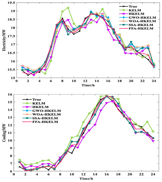
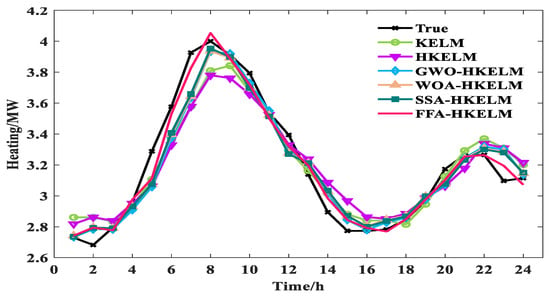
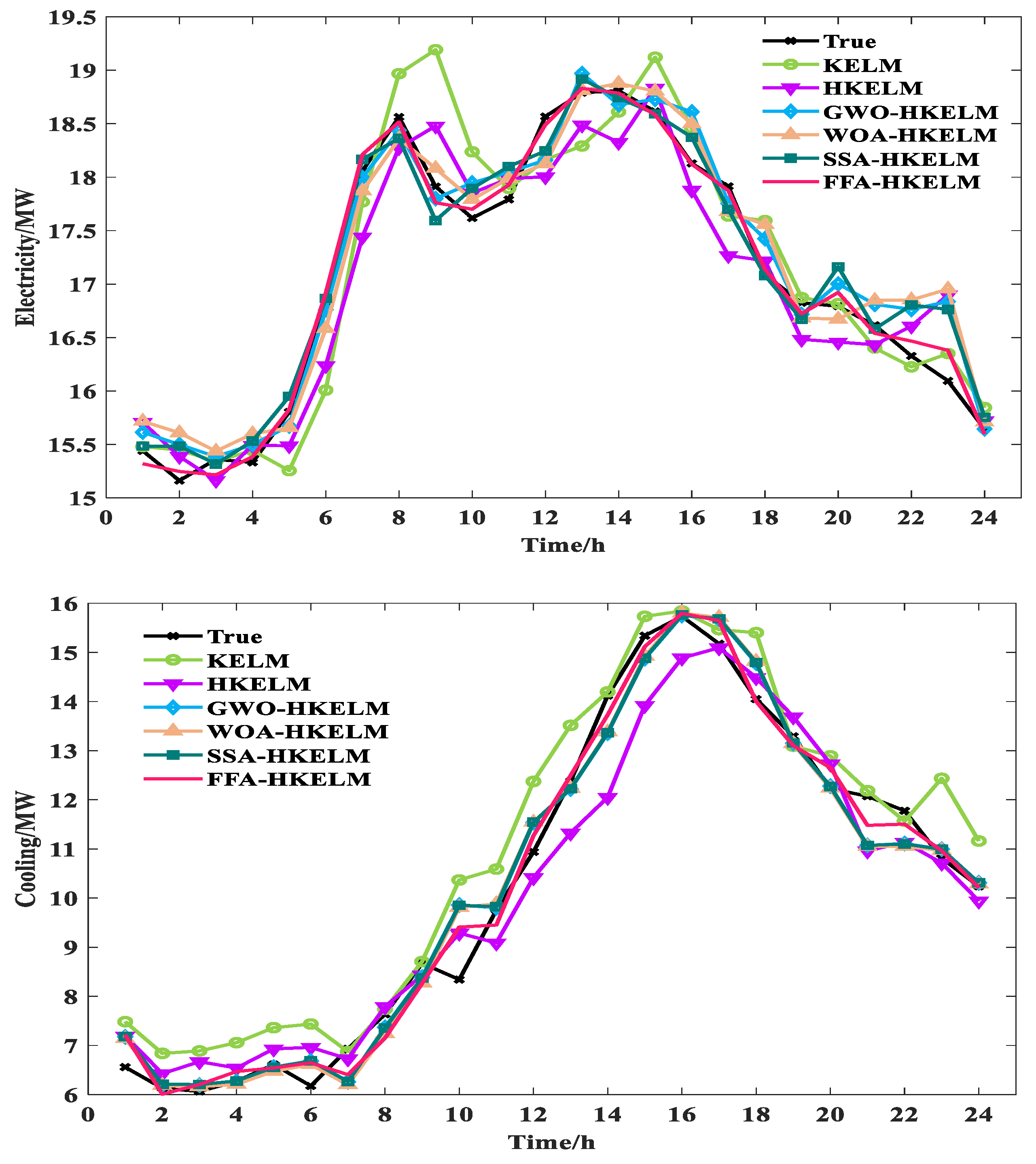
Figure 8.
Model prediction result curves of electrical, cooling and heating loads.
From Figure 8, it can be found that for electric, heating and cooling loads, the predicted values of the proposed model are more consistent with the real values and have the best prediction precision in comparison with the other models.
Here, the FFA-HKELM model proposed in this paper is compared with the results of three traditional models, and the error indicator histograms of the results of electric, heating and cooling loads are shown in Figure 9. It can be observed that this model has the best predictive effect for electric heating and cooling loads, and obtains the smallest RMSE and MAPE value.
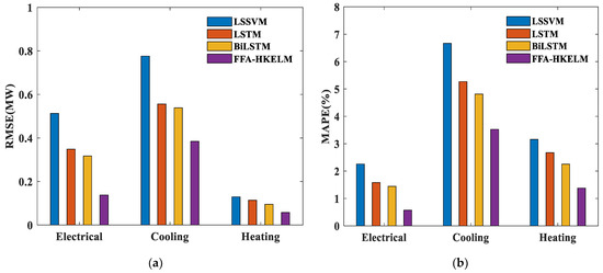
Figure 9.
(a) RMSE of the FFA-HKELM model and three traditional models; (b) MAPE of the FFA-HKELM model and three traditional models.
4.5. Analysis of Application Scale
The model in this article mainly uses historical load data and local meteorological data for prediction, which has a certain universality. In different application scenarios, anyone with the above data can use this model for prediction. In order to investigate the prediction performance of the model at different scales, this study also selected an industrial park and a residential area as two representative scenarios for prediction. The results of the IES multi-energy load forecasting for these three different application scales are shown in Table 6, in which the scale of the residential area is the smallest.
Table 6.
Prediction error results of different scales.
It can be seen from Table 6 that the model has good prediction accuracy when applied to three different scales of prediction. The model has the smallest error in IES multi-energy load forecasting for the residential area. This means that the smaller the scale of the application of the method, the better its prediction performance and exhibits higher accuracy.
5. Conclusions
This article presents a multivariate load forecasting method that employs the FFA-HKELM model to address the challenges of predicting electric, cooling and heating loads in an IES. It integrates the impact of various meteorological factors, enhancing the accuracy and reliability of the forecasting process. The actual operating data of energy stations in the Tempe area of the USA are utilized for application analysis. Different comparative experiments fully validate its effectiveness in multivariate load forecasting. Firstly, the comprehensive weight method combined with the entropy weight method and Pearson correlation coefficient is used to make the feature selection more effective and interpretable. This method can comprehensively measure the contribution degree and importance of features, and reduce the influence of subjective judgment and uncertainty. The model selects features that have a stronger correlation and higher information content by comprehensively considering various factors. This approach enhances the accuracy and reliability of the feature selection, thereby improving the model’s overall predictive performance. The mixed kernel function of this model not only improves the local search capability, but also enhances the global search capability indirectly through the linearly weighted Ploy kernel function and RBF kernel function. At the same time, the FFA algorithm can optimize the key penalty parameters and kernel parameters, and increase the precision of multiple load prediction. Finally, for the predicted values of electric, heating and cooling loads, the MAPE of the model is 24%~46%, 45%~74%, 43%~64% of the comparison model, severally. And under the same conditions, the MAE and RMSE of the proposed FFA-HKELM model are lower than the other models.
However, due to the limitations of data acquisition, different types of characteristic elements are not fully taken into consideration. Therefore, future studies can further consider other potential influencing factors, such as electricity demand response, prices of different energy sources and local economic material conditions, and add them to the overall forecast analysis. By measuring the degree of relevance between these factors and loads, the richness of the input features can be increased to achieve further improvements in the precision of IES multi-energy load forecasting in pursuit of broader applicability. The method presented in this paper has excellent prediction accuracy for time-varying loads such as electricity, cooling and heating. In the following research, more effective prediction methods can be proposed for random loads with temporal and spatial characteristics such as electric vehicles. This article provides a new research framework for IES multi-energy load prediction. However, due to limitations in data availability and the choice of research scenarios, this study does not consider the impact of random fluctuations from electric vehicles and distributed energy resources on the performance of load forecasting. Future work will further explore methods to enhance the performance of IES multi-energy load forecasting under conditions of multiple uncertainties.
Author Contributions
Software, Y.S.; Conceptualization, Y.S.; Writing—original draft, Y.S.; Visualization, D.L.; Data curation, D.L.; Supervision, W.W.; Writing—review and editing, W.W. All authors have read and agreed to the published version of the manuscript.
Funding
This work was supported by “the 14th Five Year Plan” Hubei Provincial advantaged characteristic disciplines (groups) project of Wuhan University of Science and Technology (2023C0204).
Institutional Review Board Statement
Not applicable.
Data Availability Statement
The data presented in this study are available on request from the corresponding author.
Conflicts of Interest
The authors declare no conflicts of interest.
References
- Mazzoni, S.; Ooi, S.; Nastasi, B.; Romagnoli, A. Energy storage technologies as techno-economic parameters for master-planning and optimal dispatch in smart multi energy systems. Appl. Energy 2019, 254, 113682. [Google Scholar] [CrossRef]
- Bartolini, A.; Mazzoni, S.; Comodi, G.; Romagnoli, A. Impact of carbon pricing on distributed energy systems planning. Appl. Energy 2021, 301, 117324. [Google Scholar] [CrossRef]
- Nastasi, B.; Mazzoni, S.; Groppi, D.; Romagnoli, A.; Garcia, D.A. Optimized integration of Hydrogen technologies in Island energy systems. Renew. Energy 2021, 174, 850–864. [Google Scholar] [CrossRef]
- Wang, Y.; Wang, Y.; Huang, Y.; Li, F.; Zeng, M.; Li, J.; Wang, X.; Zhang, F. Planning and operation method of the regional integrated energy system considering economy and environment. Energy 2019, 171, 731–750. [Google Scholar] [CrossRef]
- Wang, S.; Wang, S.; Chen, H.; Gu, Q. Multi-energy load forecasting for regional integrated energy systems considering temporal dynamic and coupling characteristics. Energy 2020, 195, 116964. [Google Scholar] [CrossRef]
- Jahanbin, A.; Abdolmaleki, L.; Berardi, U. Techno-economic feasibility of integrating hybrid-battery hydrogen energy storage in academic buildings. Energy Convers. Manag. 2024, 309, 118445. [Google Scholar] [CrossRef]
- Zhou, X.; Feng, C. The impact of environmental regulation on fossil energy consumption in China: Direct and indirect effects. J. Clean. Prod. 2017, 142, 3174–3183. [Google Scholar] [CrossRef]
- Jahani, A.; Zare, K.; Khanli, L.M. Short-term load forecasting for microgrid energy management system using hybrid SPM-LSTM. Sustain. Cities Soc. 2023, 98, 104775. [Google Scholar] [CrossRef]
- Zulfiqar, M.; Kamran, M.; Rasheed, M.B.; Alquthami, T.; Milyani, A.H. A hybrid framework for short term load forecasting with a navel feature engineering and adaptive grasshopper optimization in smart grid. Appl. Energy 2023, 338, 120829. [Google Scholar] [CrossRef]
- Liu, Z.; Cui, Y.; Wang, J.; Yue, C.; Agbodjan, Y.S.; Yang, Y. Multi-objective optimization of multi-energy complementary integrated energy systems considering load prediction and renewable energy production uncertainties. Energy 2022, 254, 124399. [Google Scholar] [CrossRef]
- Song, K.B.; Kwon, O.S.; Park, J.D. Optimal coefficient selection of exponential smoothing model in short term load forecasting on weekdays. Trans. Korean Inst. Electr. Eng. 2013, 62, 149–154. [Google Scholar] [CrossRef]
- Nigitz, T.; Gölles, M. A generally applicable, simple and adaptive forecasting method for the short-term heat load of consumers. Appl. Energy 2019, 241, 73–81. [Google Scholar] [CrossRef]
- Amini, M.H.; Kargarian, A.; Karabasoglu, O. ARIMA-based decoupled time series forecasting of electric vehicle charging demand for stochastic power system operation. Electr. Power Syst. Res. 2016, 140, 378–390. [Google Scholar] [CrossRef]
- Takeda, H.; Tamura, Y.; Sato, S. Using the ensemble Kalman filter for electricity load forecasting and analysis. Energy 2016, 104, 184–198. [Google Scholar] [CrossRef]
- Ali, M.; Adnan, M.; Tariq, M.; Poor, H.V. Load forecasting through estimated parametrized based fuzzy inference system in smart grids. IEEE Trans. Fuzzy Syst. 2020, 29, 156–165. [Google Scholar] [CrossRef]
- Li, Y.; Wen, Z.; Cao, Y.; Tan, Y.; Sidorov, D.; Panasetsky, D. A combined forecasting approach with model self-adjustment for renewable generations and energy loads in smart community. Energy 2017, 129, 216–227. [Google Scholar] [CrossRef]
- Heydari, A.; Nezhad, M.M.; Pirshayan, E.; Garcia, D.A.; Keynia, F.; De Santoli, L. Short-term electricity price and load forecasting in isolated power grids based on composite neural network and gravitational search optimization algorithm. Appl. Energy 2020, 277, 115503. [Google Scholar] [CrossRef]
- Eskandari, H.; Imani, M.; Moghaddam, M.P. Convolutional and recurrent neural network based model for short-term load forecasting. Electr. Power Syst. Res. 2021, 195, 107173. [Google Scholar] [CrossRef]
- Kim, J.; Moon, J.; Hwang, E.; Kang, P. Recurrent inception convolution neural network for multi short-term load forecasting. Energy Build. 2019, 194, 328–341. [Google Scholar] [CrossRef]
- Wang, F.; Xuan, Z.; Zhen, Z.; Li, K.; Wang, T.; Shi, M. A day-ahead PV power forecasting method based on LSTM-RNN model and time correlation modification under partial daily pattern prediction framework. Energy Convers. Manag. 2020, 212, 112766. [Google Scholar] [CrossRef]
- Sekhar, C.; Dahiya, R. Robust framework based on hybrid deep learning approach for short term load forecasting of building electricity demand. Energy 2023, 268, 126660. [Google Scholar] [CrossRef]
- Sun, Q.; Wang, X.; Zhang, Y.; Zhang, F.; Zhang, P.; Gao, W. Multiple load prediction of integrated energy system based on long short-term memory and multi-task learning. Autom. Electr. Power Syst. 2021, 45, 63–70. [Google Scholar]
- Zhang, G.; Bai, X.; Wang, Y. Short-time multi-energy load forecasting method based on CNN-Seq2Seq model with attention mechanism. Mach. Learn. Appl. 2021, 5, 100064. [Google Scholar] [CrossRef]
- Niu, D.; Yu, M.; Sun, L.; Gao, T.; Wang, K. Short-term multi-energy load forecasting for integrated energy systems based on CNN-BiGRU optimized by attention mechanism. Appl. Energy 2022, 313, 118801. [Google Scholar] [CrossRef]
- Wang, X.; Wang, S.; Zhao, Q.; Wang, S.; Fu, L. A multi-energy load prediction model based on deep multi-task learning and ensemble approach for regional integrated energy systems. Int. J. Electr. Power Energy Syst. 2021, 126, 106583. [Google Scholar]
- Zhu, R.; Guo, W.; Gong, X. Short-term load forecasting for CCHP systems considering the correlation between heating, gas and electrical loads based on deep learning. Energies 2019, 12, 3308. [Google Scholar] [CrossRef]
- Casanova, R.H.; Conde, A. Enhancement of LSTM models based on data pre-processing and optimization of Bayesian hyperparameters for day-ahead photovoltaic generation prediction. Comput. Electr. Eng. 2024, 116, 109162. [Google Scholar] [CrossRef]
- Jeddi, S.; Sharifian, S. A hybrid wavelet decomposer and GMDH-ELM ensemble model for Network function virtualization workload forecasting in cloud computing. Appl. Soft Comput. 2020, 88, 105940. [Google Scholar] [CrossRef]
- Loizidis, S.; Kyprianou, A.; George, G.E. Electricity market price forecasting using ELM and Bootstrap analysis: A case study of the German and Finnish Day-Ahead markets. Appl. Energy 2024, 363, 123058. [Google Scholar] [CrossRef]
- Gaspar, A.; Oliva, D.; Hinojosa, S.; Aranguren, I.; Zaldivar, D. An optimized Kernel Extreme Learning Machine for the classification of the autism spectrum disorder by using gaze tracking images. Appl. Soft Comput. 2022, 120, 108654. [Google Scholar] [CrossRef]
- Leng, J.; Incecik, A.; Wang, M.; Feng, S.; Li, Y.; Yang, C.; Li, Z. Damage detection of offshore jacket structures using structural vibration measurements: Application of a new hybrid machine learning method. Ocean. Eng. 2023, 288, 116078. [Google Scholar] [CrossRef]
- Cheng, M.; Jiao, L.; Yan, P.; Li, S.; Dai, Z.; Qiu, T.; Wang, X. Prediction and evaluation of surface roughness with hybrid kernel extreme learning machine and monitored tool wear. J. Manuf. Process. 2022, 84, 1541–1556. [Google Scholar] [CrossRef]
- Wang, S.; Liu, Z.; Jia, Z.; Li, Z. Incipient fault diagnosis of analog circuit with ensemble HKELM based on fused multi-channel and multi-scale features. Eng. Appl. Artif. Intell. 2023, 117, 105633. [Google Scholar] [CrossRef]
- Bai, L.; Liu, Z.; Wang, J. Novel hybrid extreme learning machine and multi-objective optimization algorithm for air pollution prediction. Appl. Math. Model. 2022, 106, 177–198. [Google Scholar] [CrossRef]
- Xu, X.; Zhang, T.; Qiu, Z.; Gao, H.; Zhu, S. A Method Based on NGO-HKELM for the Autonomous Diagnosis of Semiconductor Power Switch Open-Circuit Faults in Three-Phase Grid-Connected Photovoltaic Inverters. Sustainability 2023, 15, 9588. [Google Scholar] [CrossRef]
- Fan, J.; Wang, X.; Xu, H. Prediction method of tectonic coal thickness based on particle swarm optimized hybrid kernel extreme learning machine. J. Comput. Appl. 2018, 38, 1820. [Google Scholar]
- Arsene, C.; Parisio, A. Deep convolutional neural networks for short-term multi-energy demand prediction of integrated energy systems. Int. J. Electr. Power Energy Syst. 2024, 160, 110111. [Google Scholar] [CrossRef]
- Liu, H.; Tang, Y.; Pu, Y.; Mei, F.; Sidorov, D. Short-term load forecasting of multi-energy in integrated energy system based on multivariate phase space reconstruction and support vector regression mode. Electr. Power Syst. Res. 2022, 210, 108066. [Google Scholar] [CrossRef]
- Trojovská, E.; Dehghani, M.; Trojovský, P. Fennec fox optimization: A new nature-inspired optimization algorithm. IEEE Access 2022, 10, 84417–84443. [Google Scholar] [CrossRef]
- Mirjalili, S.; Mirjalili, S.M.; Lewis, A. Grey wolf optimizer. Adv. Eng. Softw. 2014, 69, 46–61. [Google Scholar] [CrossRef]
- Mirjalili, S.; Lewis, A. The whale optimization algorithm. Adv. Eng. Softw. 2016, 95, 51–67. [Google Scholar] [CrossRef]
- Xue, J.; Shen, B. A novel swarm intelligence optimization approach: Sparrow search algorithm. Syst. Sci. Control. Eng. 2020, 8, 22–34. [Google Scholar] [CrossRef]
- AUS Campus Metabolism. Available online: https://cm.asu.edu/ (accessed on 12 November 2023).


Disclaimer/Publisher’s Note: The statements, opinions and data contained in all publications are solely those of the individual author(s) and contributor(s) and not of MDPI and/or the editor(s). MDPI and/or the editor(s) disclaim responsibility for any injury to people or property resulting from any ideas, methods, instructions or products referred to in the content. |
© 2024 by the authors. Licensee MDPI, Basel, Switzerland. This article is an open access article distributed under the terms and conditions of the Creative Commons Attribution (CC BY) license (https://creativecommons.org/licenses/by/4.0/).