
Prognostic Properties of Instantaneous Amplitudes Maxima of Earth Surface Tremor

Abstract
1. Introduction
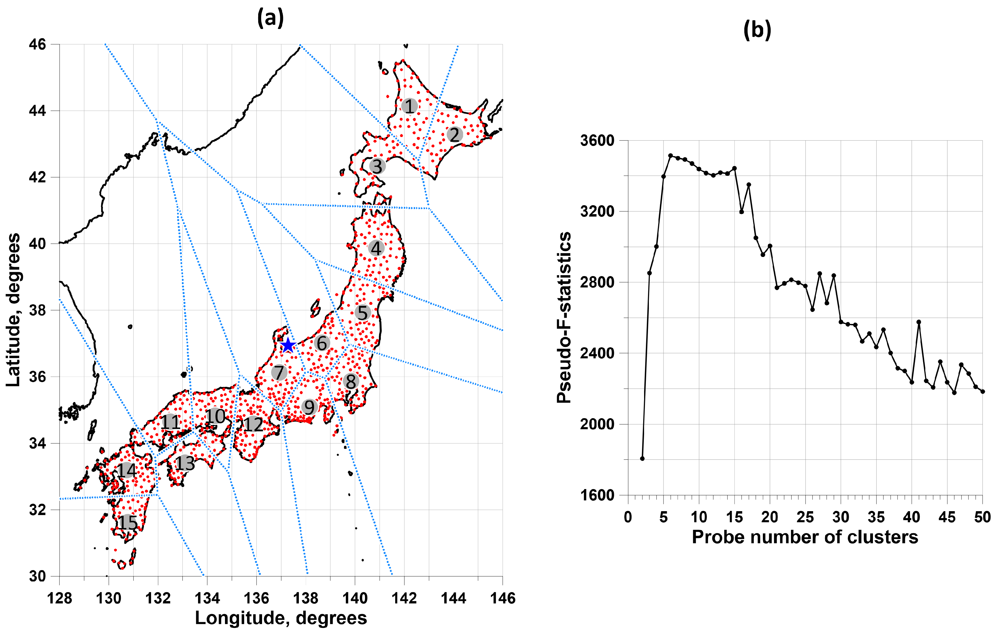
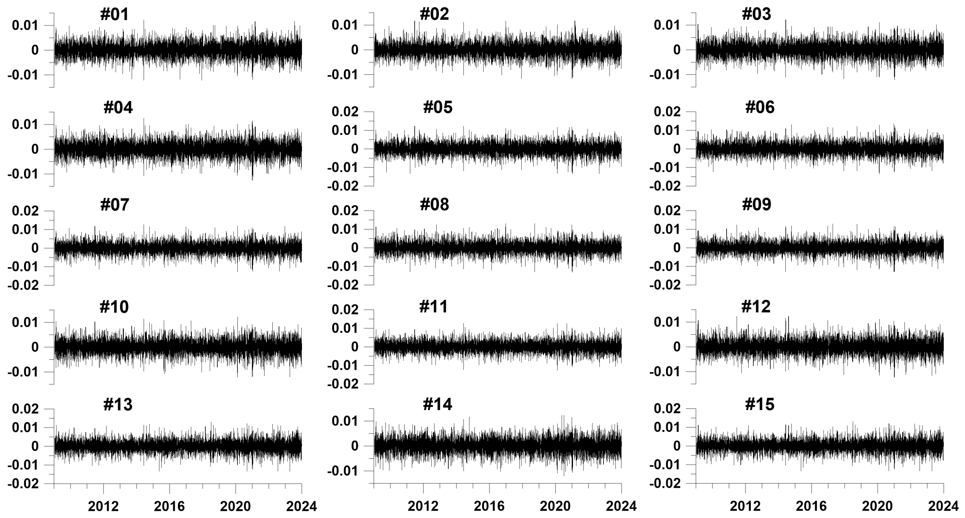
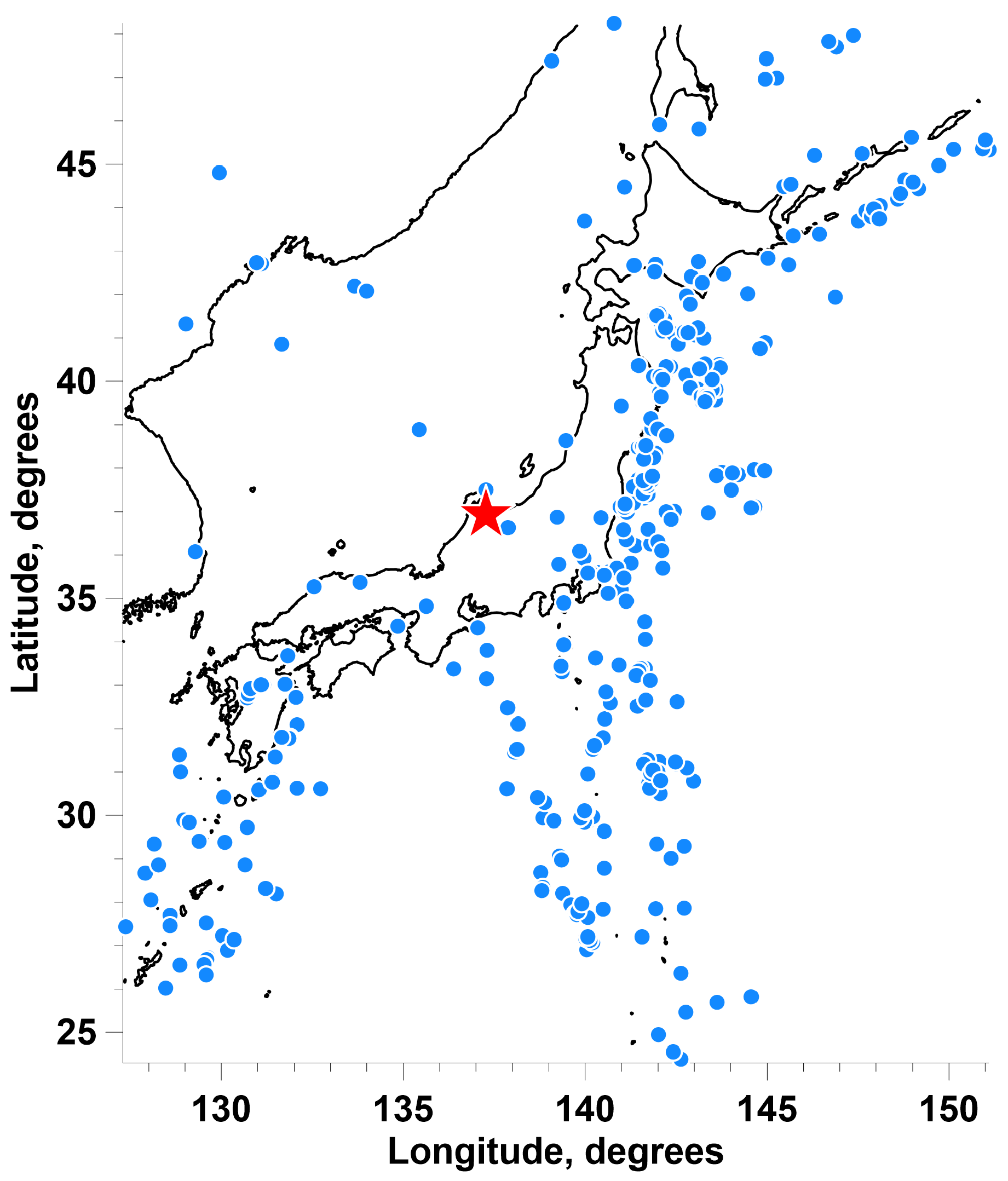
2. Data
3. Principal Components of Increments in a Moving Time Window
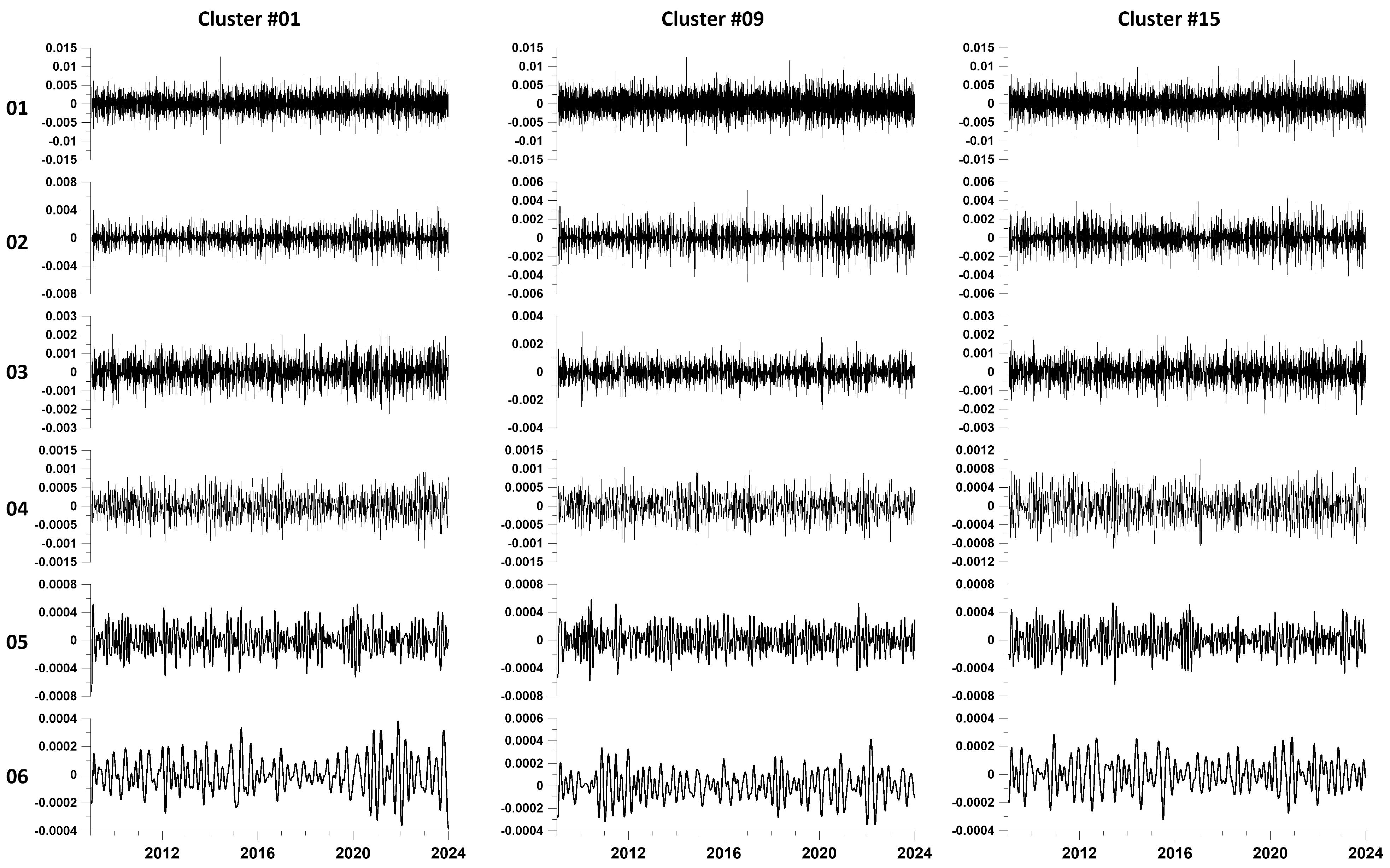
4. Empirical Mode Decomposition
5. Ensemble Empirical Mode Decomposition
- Add a white noise implementation to the original data.
- Decomposition of data with the addition of white noise into empirical modes.
- Repeat steps 1 and 2 quite a large number of times with different implementations of white noise.
- Obtain the ensemble average for the corresponding empirical modes.
6. Hilbert Transform
7. Influence Matrix
- (1)
- a sequence of moments in time corresponding to the largest local maxima of the amplitudes of the envelopes at certain levels of the EEMD Huang decomposition
- (2)
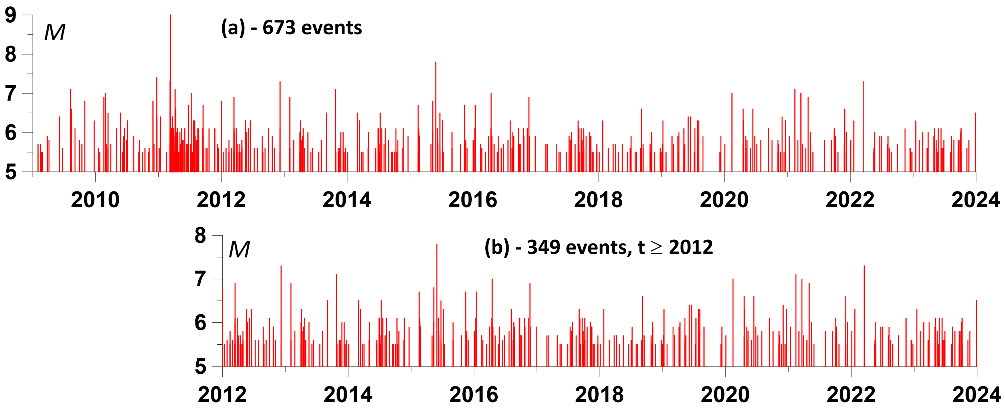
- a sequence of times of seismic events with a magnitude not less than a given value.
8. Estimation of Connections between the Times of Local Amplitude Maxima and Seismic Events
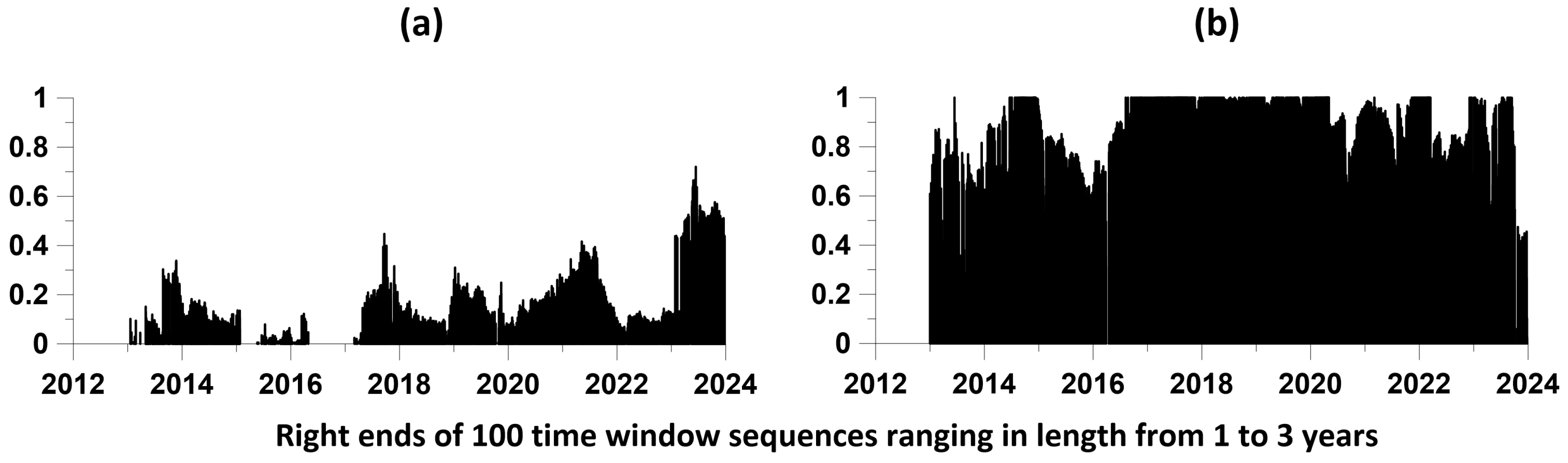
- The minimum and maximum lengths of time windows and —the number of lengths of time windows in this interval are selected. Thus, the lengths of the time windows took on the values , , . In our calculations, we took as equal to 1 year, and —3 years, .
- Each time window of length was shifted from left to right along the time axis with some offset . Let us denote by , the sequence of moments in time of the positions of the right windows with length . The number of time windows in length is determined by their time offset . We used a time window offset of 0.01 year.
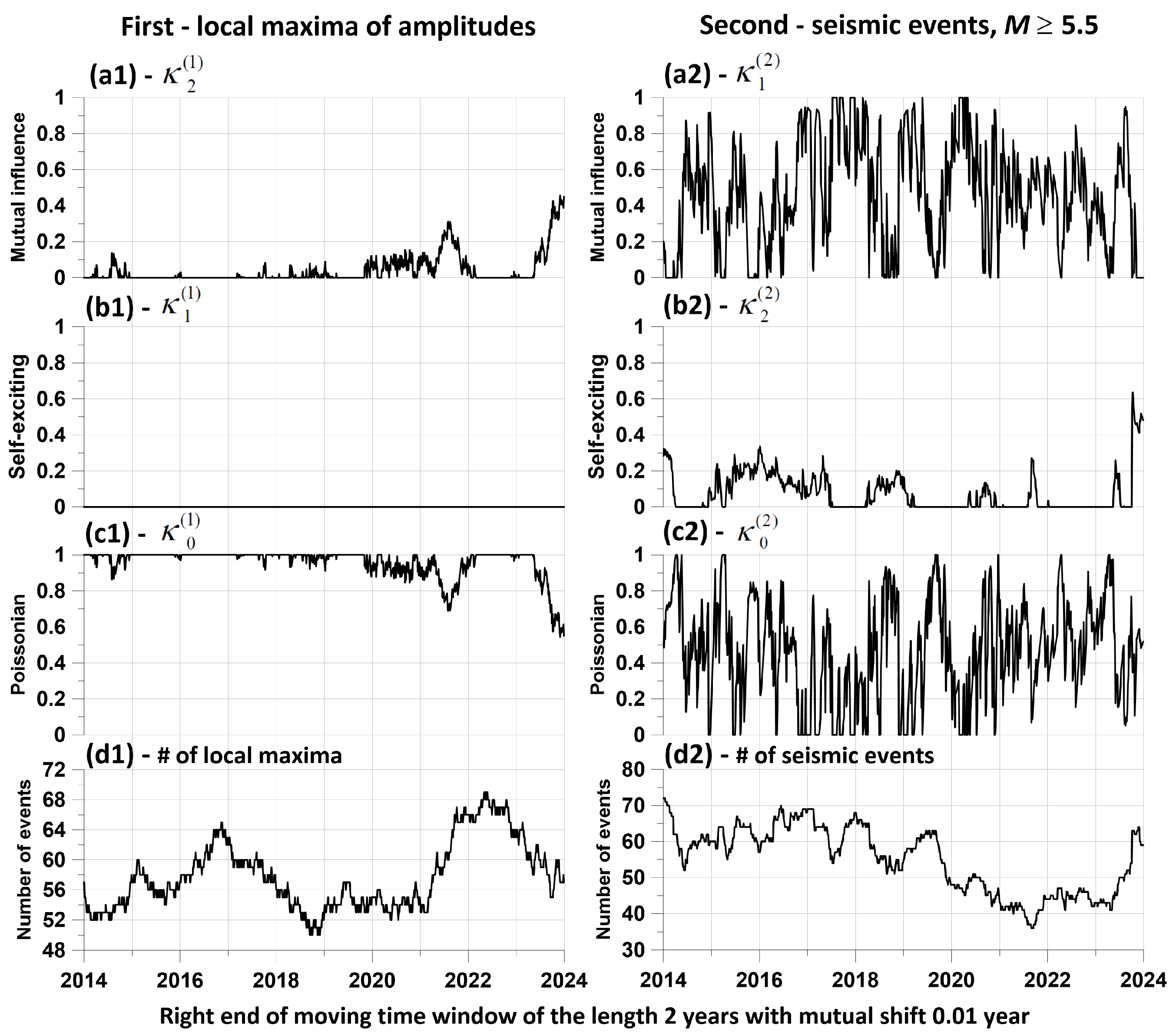
- For each position of a time window of length , the elements of the influence matrix (35) are estimated for a given relaxation time of the model (26–27), corresponding to the mutual influence of the two processes being analyzed. We took a value equal to 0.1 year. For definiteness, we will consider one influence, for example, of the first process on the second. As a result of such estimates, we obtain their values in the form , where is the corresponding element of the influence matrix for a position with a time window number of length .
- In the sequence , we select elements corresponding to local maxima of values , that is, from the condition . Let us present each element as a vertical segment of length located at a time point . The combination of such vertical graphic elements for all , visualizes the “strength” of the mutual influence of processes on each other.
9. Conclusions
Author Contributions
Funding
Institutional Review Board Statement
Data Availability Statement
Acknowledgments
Conflicts of Interest
References
- Lyubushin, A. Identification of Areas of Anomalous Tremor of the Earth’s Surface on the Japanese Islands According to GPS Data. Appl. Sci. 2022, 12, 7297. [Google Scholar] [CrossRef]
- Lyubushin, A. Singular Points of the Tremor of the Earth’s Surface. Appl. Sci. 2023, 13, 10060. [Google Scholar] [CrossRef]
- Lyubushin, A. Entropy of GPS-measured Earth tremor. In Revolutionizing Earth Observation—New Technologies and Insights; Abdalla, R.M., Ed.; IntechOpen: Rijeka, Croatia, 2024. [Google Scholar] [CrossRef]
- Lyubushin, A. Global coherence of GPS-measured high-frequency surface tremor motions. GPS Solut. 2018, 22, 116. [Google Scholar] [CrossRef]
- Lyubushin, A. Field of coherence of GPS-measured earth tremors. GPS Solut. 2019, 23, 120. [Google Scholar] [CrossRef]
- Filatov, D.M.; Lyubushin, A.A. Fractal analysis of GPS time series for early detection of disastrous seismic events. Phys. A Stat. Mech. Its Appl. 2017, 469, 718–730. [Google Scholar] [CrossRef]
- Filatov, D.M.; Lyubushin, A.A. Precursory Analysis of GPS Time Series for Seismic Hazard Assessment. Pure Appl. Geophys. 2019, 177, 509–530. [Google Scholar] [CrossRef]
- Huang, N.E.; Shen, Z.; Long, S.R.; Wu, V.C.; Shih, H.H.; Zheng, Q.; Yen, N.C.; Tung, C.C.; Liv, H.H. The empirical mode decomposition and the Hilbert spectrum for nonlinear and non-stationary time series analysis. Proc. R. Soc. Lond. Ser. A 1998, 454, 903–995. [Google Scholar] [CrossRef]
- Huang, N.E.; Wu, Z. A review on Hilbert-Huang transform: Method and its applications to geophysical studies. Rev. Geophys. 2008, 46, RG2006. [Google Scholar] [CrossRef]
- Pan, Y.; Shen, W.-B.; Ding, H.; Hwang, C.; Li, J.; Zhang, T. The Quasi-Biennial Vertical Oscillations at Ghlobal GPS Stations: Identification by Ensemble Empirical Mode Decomposition. Sensors 2015, 15, 26096–26114. [Google Scholar] [CrossRef]
- Li, W.; Guo, J. Extraction of periodic signals in Global Navigation Satellite System (GNSS) vertical coordinate time series using the adaptive ensemble empirical modal decomposition method. Nonlin. Process. Geophys. 2024, 31, 99–113. [Google Scholar] [CrossRef]
- Huang, Y.; Schmitt, F.G.; Lu, Z.; Liu, Y. Analysis of daily river flow fluctuations using empirical mode decomposition and arbitrary order Hilbert spectral analysis. J. Hydrol. 2009, 373, 103–111. [Google Scholar] [CrossRef]
- Huang, N.E.; Wu, M.; Qu, W.; Long, S.R.; Shen, S.S.P. Applications of Hilbert–Huang transform to non-stationary financial time series analysis. Appl. Stoch. Models Bus. Ind. 2003, 19, 245–268. [Google Scholar] [CrossRef]
- Li, H.; Kwong, S.; Yang, L.; Huang, D.; Xiao, D. Hilbert-Huang Transform for Analysis of Heart Rate Variability in Cardiac Health. IEEE/ACM Trans. Comput. Biol. Bioinform. 2011, 8, 1557–1567. [Google Scholar] [CrossRef]
- Wei, H.-C.; Xiao, M.-X.; Chen, H.-Y.; Li, Y.-Q.; Wu, H.-T.; Sun, C.-K. Instantaneous frequency from Hilbert-Huang transformation of digital volume pulse as indicator of diabetes and arterial stiffness in upper-middle-aged subjects. Sci. Rep. 2018, 8, 15771. [Google Scholar] [CrossRef] [PubMed]
- Sarlis, N.V.; Skordas, E.S.; Mintzelas, A.; Papadopoulou, K.A. Micro-scale, mid-scale, and macro-scale in global seismicity identified by empirical mode decomposition and their multifractal characteristics. Sci. Rep. 2018, 8, 9206. [Google Scholar] [CrossRef]
- Beavan, J. Noise properties of continuous GPS data from concrete pillar geodetic monuments in New Zealand and comparison with data from U.S. deep drilled braced monuments. J. Geophys. Res. 2005, 110, B08. [Google Scholar] [CrossRef]
- Langbein, J. Noise in GPS displacement measurements from Southern California and Southern Nevada. J. Geophys. Res. 2008, 113, B05405. [Google Scholar] [CrossRef]
- Blewitt, G.; Lavallee, D. Effects of annual signal on geodetic velocity. J. Geophys. Res. 2002, 107, 2145. [Google Scholar] [CrossRef]
- Bos, M.S.; Fernandes, R.M.S.; Williams, S.D.P.; Bastos, L. Fast error analysis of continuous GPS observations. J. Geod. 2008, 82, 157–166. [Google Scholar] [CrossRef]
- Liu, B.; Xing, X.; Tan, J.; Xia, Q. Modeling Seasonal Variations in Vertical GPS Coordinate Time Series Using Independent Component Analysis and Varying Coefficient Regression. Sensors 2020, 20, 5627. [Google Scholar] [CrossRef]
- Liu, B.; Dai, W.; Liu, N. Extracting seasonal deformations of the Nepal Himalaya region from vertical GPS position time series using Independent Component Analysis. Adv. Space Res. 2017, 60, 2910–2917. [Google Scholar] [CrossRef]
- Tesmer, V.; Steigenberger, P.; van Dam, T.; Mayer-Gurr, T. Vertical deformations from homogeneously processed GRACE and global GPS long-term series. J. Geod. 2011, 85, 291–310. [Google Scholar] [CrossRef]
- Yan, J.; Dong, D.; Burgmann, R.; Materna, K.; Tan, W.; Peng, Y.; Chen, J. Separation of Sources of Seasonal Uplift in China Using Independent Component Analysis of GNSS Time Series. J. Geophys. Res. Solid Earth 2019, 124, 11951–11971. [Google Scholar] [CrossRef]
- Santamaría-Gómez, A.; Memin, A. Geodetic secular velocity errors due to interannual surface loading deformation. Geophys. J. Int. 2015, 202, 763–767. [Google Scholar] [CrossRef]
- Fu, Y.; Argus, D.F.; Freymueller, J.T.; Heflin, M.B. Horizontal motion in elastic response to seasonal loading of rain water in the Amazon Basin and monsoon water in Southeast Asia observed by GPS and inferred from GRACE. Geophys. Res. Lett. 2013, 40, 6048–6053. [Google Scholar] [CrossRef]
- Chanard, K.; Avouac, J.P.; Ramillien, G.; Genrich, J. Modeling deformation induced by seasonal variations of continental water in the Himalaya region: Sensitivity to Earth elastic structure. J. Geophys. Res. Solid Earth 2014, 119, 5097–5113. [Google Scholar] [CrossRef]
- He, X.; Montillet, J.P.; Fernandes, R.; Bos, M.; Yu, K.; Hua, X.; Jiang, W. Review of current GPS methodologies for producing accurate time series and their error sources. J. Geodyn. 2017, 106, 12–29. [Google Scholar] [CrossRef]
- Ray, J.; Altamimi, Z.; Collilieux, X.; van Dam, T. Anomalous harmonics in the spectra of GPS position estimates. GPS Solut. 2008, 12, 55–64. [Google Scholar] [CrossRef]
- Roncagliolo, P.A.; García, J.G.; Mercader, P.I.; Fuhrmann, D.R.; Muravchik, C.H. Maximum-likelihood attitude estimation using GPS signals. Digit. Signal Process. 2007, 17, 1089–1100. [Google Scholar] [CrossRef]
- Wang, F.; Li, H.; Lu, M. GNSS Spoofing Detection and Mitigation Based on Maximum Likelihood Estimation. Sensors 2017, 17, 1532. [Google Scholar] [CrossRef]
- Parkinson, B.W. Global Positioning System: Theory and Applications; AIAA: Reston, VA, USA, 1996; p. 781. [Google Scholar]
- Xu, J.; He, J.; Zhang, Y.; Xu, F.; Cai, F. A Distance-Based Maximum Likelihood Estimation Method for Sensor Localization in Wireless Sensor Networks. Int. J. Distrib. Sens. Netw. 2016, 12, 2080536. [Google Scholar] [CrossRef]
- Langbein, J.; Johnson, H. Correlated errors in geodetic time series, Implications for time-dependent deformation. J. Geophys. Res. 1997, 102, 591–603. [Google Scholar] [CrossRef]
- Williams, S.D.P.; Bock, Y.; Fang, P.; Jamason, P.; Nikolaidis, R.M.; Prawirodirdjo, L.; Miller, M.; Johnson, D.J. Error analysis of continuous GPS time series. J. Geophys. Res. 2004, 109, B03412. [Google Scholar] [CrossRef]
- Wang, W.; Zhao, B.; Wang, Q.; Yang, S. Noise analysis of continuous GPS coordinate time series for CMONOC. Adv. Space Res. 2012, 49, 943–956. [Google Scholar] [CrossRef]
- Agnew, D. The time domain behavior of power law noises. Geophys. Res. Lett. 1992, 19, 333–336. [Google Scholar] [CrossRef]
- Amiri-Simkooei, A.R.; Tiberius, C.C.J.M.; Teunissen, P.J.G. Teunissen Assessment of noise in GPS coordinate time series: Methodology and results. J. Geophys. Res. 2007, 112, B07413. [Google Scholar] [CrossRef]
- Caporali, A. Average strain rate in the Italian crust inferred from a permanent GPS network—I. Statistical analysis of the time-series of permanent GPS stations. Geophys. J. Int. 2003, 155, 241–253. [Google Scholar] [CrossRef]
- Zhang, J.; Bock, Y.; Johnson, H.; Fang, P.; Williams, S.; Genrich, J.; Wdowinski, S.; Behr, J. Southern California permanent GPS geodetic array: Error analysis of daily position estimates and site velocities. J. Geophys. Res. 1997, 102, 18035–18055. [Google Scholar] [CrossRef]
- Li, J.; Miyashita, K.; Kato, T.; Miyazaki, S. GPS time series modeling by autoregressive moving average method, Application to the crustal deformation in central Japan. Earth Planets Space 2000, 52, 155–162. [Google Scholar] [CrossRef]
- Kermarrec, G.; Schon, S. On modelling GPS phase correlations: A parametric model. Acta Geod. Geophys. 2018, 53, 139–156. [Google Scholar] [CrossRef]
- Teferle, F.N.; Williams, S.D.P.; Kierulf, H.P.; Bingley, R.M.; Plag, H.P. A continuous GPS coordinate time series analysis strategy for high-accuracy vertical land movements. Phys. Chem. Earth Parts A/B/C 2008, 33, 205–216. [Google Scholar] [CrossRef]
- Chen, Q.; van Dam, T.; Sneeuw, N.; Collilieux, X.; Weigelt, M.; Rebischung, P. Singular spectrum analysis for modeling seasonal signals from GPS time series. J. Geodyn. 2013, 72, 25–35. [Google Scholar] [CrossRef]
- Bock, Y.; Melgar, D.; Crowell, B.W. Real-Time Strong-Motion Broadband Displacements from Collocated GPS and Accelerometers. Bull. Seismol. Soc. Am. 2011, 101, 2904–2925. [Google Scholar] [CrossRef]
- Goudarzi, M.A.; Cocard, M.; Santerre, R.; Woldai, T. GPS interactive time series analysis software. GPS Solut. 2013, 17, 595–603. [Google Scholar] [CrossRef]
- Hackl, M.; Malservisi, R.; Hugentobler, U.; Jiang, Y. Velocity covariance in the presence of anisotropic time correlated noise and transient events in GPS time series. J. Geodyn. 2013, 72, 36–45. [Google Scholar] [CrossRef]
- Khelif, S.; Kahlouche, S.; Belbachir, M.F. Analysis of position time series of GPS-DORIS co-located stations. Int. J. Appl. Earth Observ. Geoinf. 2013, 20, 67–76. [Google Scholar] [CrossRef]
- Blewitt, G.; Hammond, W.C.; Kreemer, C. Harnessing the GPS data explosion for interdisciplinary science. Eos 2018, 99, 485. [Google Scholar] [CrossRef]
- Duda, R.O.; Hart, P.E.; Stork, D.G. Pattern Classification; Wiley: Hoboken, NJ, USA, 2000. [Google Scholar]
- Vogel, M.A.; Wong, A.K.C. PFS clustering method. IEEE Trans. Pattern Anal. Mach. Intell. 1979, 1, 237–245. [Google Scholar] [CrossRef] [PubMed]
- Jolliffe, I.T. Principal Component Analysis; Springer: Berlin/Heidelberg, Germany, 1986. [Google Scholar]
- Huber, P.J. Robust Statistics; Wiley: Toronto, ON, Canada; Chichester, UK; New York, NY, USA, 1981. [Google Scholar]
- Bendat, J.S.; Piersol, A.G. Random Data. Analysis and Measurement Procedures, 4th ed.; Wiley & Sons: Hoboken, NJ, USA, 2010. [Google Scholar]
- Lyubushin, A. Investigation of the Global Seismic Noise Properties in Connection to Strong Earthquakes. Front. Earth Sci. 2022, 10, 905663. [Google Scholar] [CrossRef]
- Lyubushin, A. Seismic Hazard Indicators in Japan based on Seismic Noise Properties. J. Earth Environ. Sci. Res. 2023, 5, 1–8. [Google Scholar] [CrossRef]
- Lyubushin, A.; Rodionov, E. Wavelet-based correlations of the global magnetic field in connection to strongest earthquakes. Adv. Space Res. 2024. [Google Scholar] [CrossRef]
- Cox, D.R.; Lewis, P.A.W. The Statistical Analysis of Series of Events; Methuen: London, UK, 1966. [Google Scholar]
- Varotsos, P.A.; Sarlis, N.V.; Skordas, E.S.; Toshiyasu, N.; Masashi, K. The unusual case of the ultra-deep 2015 Ogasawara earthquake (Mw7.9): Natural time analysis. EPL 2021, 135, 49002. [Google Scholar] [CrossRef]


| Clust#. | 1 | 2 | 3 | 4 | 5 | 6 | 7 | 8 | 9 | 10 | 11 | 12 | 13 | 14 | 15 |
| Nsta | 57 | 56 | 54 | 83 | 69 | 61 | 78 | 77 | 91 | 76 | 57 | 95 | 48 | 88 | 57 |
Disclaimer/Publisher’s Note: The statements, opinions and data contained in all publications are solely those of the individual author(s) and contributor(s) and not of MDPI and/or the editor(s). MDPI and/or the editor(s) disclaim responsibility for any injury to people or property resulting from any ideas, methods, instructions or products referred to in the content. |
© 2024 by the authors. Licensee MDPI, Basel, Switzerland. This article is an open access article distributed under the terms and conditions of the Creative Commons Attribution (CC BY) license (https://creativecommons.org/licenses/by/4.0/).
Share and Cite
Lyubushin, A.; Rodionov, E. Prognostic Properties of Instantaneous Amplitudes Maxima of Earth Surface Tremor. Entropy 2024, 26, 710. https://doi.org/10.3390/e26080710
Lyubushin A, Rodionov E. Prognostic Properties of Instantaneous Amplitudes Maxima of Earth Surface Tremor. Entropy. 2024; 26(8):710. https://doi.org/10.3390/e26080710
Chicago/Turabian StyleLyubushin, Alexey, and Eugeny Rodionov. 2024. "Prognostic Properties of Instantaneous Amplitudes Maxima of Earth Surface Tremor" Entropy 26, no. 8: 710. https://doi.org/10.3390/e26080710
APA StyleLyubushin, A., & Rodionov, E. (2024). Prognostic Properties of Instantaneous Amplitudes Maxima of Earth Surface Tremor. Entropy, 26(8), 710. https://doi.org/10.3390/e26080710