On the Tripped Rollovers and Lateral Skid in Three-Wheeled Vehicles and Their Mitigation

Abstract

Active safety systems for three-wheeled vehicles seem to be in premature development; in particular, delta types, also known as tuk-tuks or sidecars, are sold with minimal protection against accidents. Unfortunately, the risk of wheel lifting and lateral and/or longitudinal vehicle roll is high. For instance, a tripped rollover occurs when a vehicle slides sideways, digging its tires into soft soil or striking an object. Unfortunately, research is mostly aimed at un-tripped rollovers while most of the rollovers are tripped. In this paper, models for lateral skid tripped and un-tripped rollover risks are presented. Later, independent braking and accelerating control actions are used to develop a dynamic stability control (DSC) to assist the driver in mitigating such risks, including holes/bumps road-scenarios. A common Lyapunov function and an LMI problem resolution ensure robust stability while optimization allows tuning the controller. Numerical and HIL tests are presented. Implementation on a three-wheeled vehicle requires an inertial measurement unit, and independent ABS and propulsion control as main components.

1. Introduction

A delta three-wheeled vehicle (in the following denoted as TWV), either with electric or combustion propulsion/traction, is cheaper for its simplicity than a tadpole-type. A TWV has two rear wheels and one at the front; tadpole-type vehicles have two front wheels and a rear-wheel, but, usually, a TWV has a simple suspension system with fixed camber and caster; tadpole configurations include costly suspension systems with variable camber/caster [1]. Unfortunately, TWVs are more prone to accidents related to their dynamic stability [2,3,4]; for instance, a TWV is more prone to suffer a tripped/un-tripped rollover (see [5] for a definition) from a sharp turn than a tadpole. Even worse, variable loading conditions have to be considered since they have a significant effect on the center of gravity position, and hence in the rollover risk.

Some studies aimed to design of the TWVs to reduce the motion-related risks [6,7,8,9,10]. However, few studies are related to the research on tripped rollovers and skids (see for instance [11,12]) and to the knowledge of the author, there are no studies that include the effects of skidding, potholes, speed bumps or exogenous vertical forces that induce various types of accidents (tripped rollovers). Furthermore, most of the related literature is geared towards internal combustion engine vehicles without a suspension system [13] and they focus solely on lateral stability (property of the TWV to impose forces to maintain the desired position) to avoid an un-tripped rollover (induced only by a steering action). High pitch angles (wheelie or stoppie), skidding risk (by low friction coefficient), bumps/holes on the road and load and tire variations, among other uncertain parameters, are ignored. Even worse, new electric in-wheel traction/propulsion systems allows improved acceleration levels increasing the risks.

In [14] static and dynamic models were developed to gain lateral rollover stability conditions that were validated experimentally on a commercial TWV; they also suggested increasing the track width and lowering the seat heights of the TWV to minimize the risk of lateral rollover (un-tripped rollover). The authors in [15] found that the TWV is more unstable (laterally) with two or more occupants, in comparison with a single one; this was attributed to the center of gravity ($CoG$) shift. They recommended enhancing the Nigerian normative to require manufacturers to comply with stricter standards before marketing these types of vehicles.

In the PhD thesis [16] and the related article [12], sliding mode controllers were presented to mitigate un-tripped rollovers by active front steering. The model developed there considers a suspension system and, in closed-loop for nominal parameters, the un-tripped rollover was mitigated for a fish-hook maneuver. Later, the rear braking was included as a control action to mitigate such rollover more effectively. Unfortunately, active steering control in a TWV is not an easy implementation task and tripped rollovers were not considered; no experimental or semi-experimental tests were shown, neither the effect of braking nor accelerating with the front wheel.

The authors of [17] proposed the calculation of the desired yaw rate, and a full-state feedback control system for the tadpole and delta TWVs; also, they compared the under-steer with the path-following behavior. However, in addition to the same disadvantages of the previously described article, it is not mentioned how the yaw moment that serves as the control input should be generated.

In [18], a re-configurable traction/braking control is developed, in addition to handling improvement, lateral stability and rollover prevention for the delta and tadpole TWVs; the control action includes the differential braking, torque vectoring or active steering; such control actions are calculated by model predictive control (MPC). Unfortunately, the modeling of the TWV did not consider a suspension system, the skid risk (tripped rollovers), the front accelerating/braking effect nor the longitudinal rollover; also, although adaptive and MPC ensure good results under fast parametric variation, exact knowledge of every parameter at all times is needed. The authors did not present implementation insights, nor experimental or semi-experimental tests and unfortunately, real-time MPC is computationally demanding, even nowadays.

Many authors set out to obtain accurate models [19,20,21,22] with improved path following [23] and performance [24], as well as to study other related topics [25,26,27,28,29]. So far, no results have been found regarding the estimation of tripped rollovers nor the lateral skid that can cause them, much less research related to their mitigation, especially for TWVs considering a suspension system.

In this paper, new risk estimation indexes are developed to predict tripped and un-tripped rollovers as well as the skidding, considering the effects of the suspension system for TWVs. Such estimations can be easily calculated in a real scenario by chassis angular measures (obtained from an accelerometer) and are validated with the support of specialized software. Further, such estimations are used to design a new dynamic stability control (DSC) to mitigate tripped and un-tripped rollovers, as well as lateral and longitudinal skid risks, by differential braking/accelerating control actions. The design considers that potholes and speed bumps exist and can greatly increase the risk of rollover. Even more, the DSC is designed by means of robust control theory, to cope with the parametric uncertainty caused by changes in the mass, in the friction coefficient and in the height of the center of gravity, among other things; for this purpose, only nominal values have to be known. Implementation is ideal for electric TWVs, since they are able to generate correcting braking/accelerating differential torques and only require chassis angular information, obtained by an inertial measurement unit (IMU). Semi experimental tests with hardware-in-the-loop are presented to validate the effectiveness of the DSC.

Unlike previous works, in this article, tripped rollovers, the skid risk, the effects of the TWV suspension, road potholes and speed bumps, and semi-experimental tests with hardware-in-the-loop (HIL) are analyzed regardless of the traction/propulsion system.

The remainder of this paper comprises the mathematical modeling of the vehicle and lateral and longitudinal rollover risks, in Section 2, along with the necessary validations. The analytic design of the DSC is presented in Section 3. Section 4 is dedicated to showing the performance evaluation of the DSC, and the final section is dedicated to providing some conclusions and future work.

2. Modeling

In this section, a rotational model of the TWV is presented; this model is obtained through the idealizations of Figure 1. The main considerations/simplifications for this modeling are:

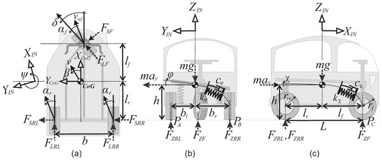
Figure 1. Idealizations and free-force diagrams for the TWV: (a) upper view, (b) back view, and (c) right view.

(i)

Only small steering angles should be demanded, for high-speed driving (16 m/s and above).

(ii)

Pitch and roll dynamics are decoupled.

(iii)

For roll dynamics, the suspension can be simplified by a single rotational spring-damper system (with $k_{\phi }$ and $c_{\phi }$ coefficients respectively), for the torque-balance about the $X_{CoG}$-axis as shown in Figure 1b.

(iv)

For pitch dynamics, the suspension can be simplified by a single rotational spring-damper system (with $k_{\mathcal{X}}$ and $c_{\mathcal{X}}$ coefficients respectively) for the torque-balance about the $Y_{CoG}$-axis as shown in Figure 1c.

Such simplifications are opportune since it is not the objective of this investigation to obtain an exact model; rather, is to obtain a conservative estimate of the rollover and skid risks in order to calculate the control actions that mitigate such risks. The robust control theory used here allows facing uncertainty in the modeling and in the parameters (with limits). In Table 1 and Table 2 are described the associated nomenclature and parameters, respectively, along with a brief description, and nominal values where applicable.

Table 1. Nomenclature.

Symbol	Description	Units
${\alpha }_f$	Front tire sideslip angle	rad
${\alpha }_r$	Rear tires sideslip angle	rad
$a_x$	CoG longitudinal acceleration	$m^2/s$
$a_y$	CoG lateral acceleration	$m^2/s$
$\beta$	CoG sideslip angle	rad
$CoG$	Center of gravity	rad
$\delta$	Front wheel angle (steer)	rad
$F_{LF}$	Front wheel longitudinal force	N
$F_{LRL}$	Rear left wheel longitudinal force	N
$F_{LRR}$	Rear right longitudinal force	N
$F_{SF}$	Front wheel lateral force	N
$F_{SRL}$	Rear left wheel lateral force	N
$F_{SRR}$	Rear right lateral force	N
$F_{ZF}$	Front wheel vertical force	N
$F_{ZRL}$	Rear left wheel vertical force	N
$F_{ZRR}$	Rear right vertical force	N
$\phi$	TWV roll angle	rad
$\psi$	TWV yaw angle	rad
$P_A$	Roll forces balance reference A	-
$P_B$	Pitch forces balance reference A	-
$\psi$	TWV yaw angle	rad
$RI$	Rollover index	-
${\mathcal{T}}_F$	Front wheel longitudinal torque	Nm
${\mathcal{T}}_{RL}$	Rear left wheel longitudinal torque	Nm
${\mathcal{T}}_{RR}$	Rear right wheel longitudinal torque	Nm
$TWV$	Three-in-wheeled electric vehicle	-
$v_{wf}$	Front wheel speed	m/s
$X_{IN}$	Inertial (fixed) longitudinal axis	-
$\mathcal{X}$	TWV pitch angle	rad
$Y_{IN}$	Inertial (fixed) lateral axis	-
$Z_{IN}$	Inertial (fixed) vertical axis	-

Table 2. Parameters.

Symbol	Description	Nominal Value	Units
b	Rear track width	$1.050$	m
$b_l$	CoG to rear left wheel distance	$0.525$	m
$b_r$	CoG to rear right wheel distance	$0.525$	m
$c_{\phi }$	Roll damper coefficient	300	Ns
$c_{\mathcal{X}}$	Pitch damper coefficient	6000	Ns
$c_f$	Front tire stiffness coefficient	25,000	N/rad
$c_r$	Rear tires (doubled) stiffness coefficient	55,000	N/rad
g	Gravity acceleration	$9.81$	$m/s^2$
h	$CoG$ height	$0.54$	m
J	Yaw moment of inertia	1111	$kg{m}^2$
$J_{\phi }$	Roll moment of inertia	288	$kg{m}^2$
$J_{\mathcal{X}}$	Pitch moment of inertia	1111	$kg{m}^2$
$k_{\phi }$	Roll spring coefficient	22,000	N
$k_{\mathcal{X}}$	Pitch spring coefficient	17,000	N
L	Front to rear axles distance	$2.025$	m
$l_f$	Front axle to $CoG$ distance	$1.103$	m
$l_r$	Rear axle to $CoG$ distance	$0.922$	m
$\mu$	Friction coefficient	$0.75$	-
m	TWV mass	747	m
$r_f$	Front wheel radius	$0.245$	m
$r_{rl}$	Rear left wheel radius	$0.245$	m
$r_{rr}$	Rear right wheel radius	$0.245$	m
v	$CoG$ speed	22	m/s

2.1. Vehicle Model

From Figure 1a and Consideration (i), longitudinal and lateral accelerations acting on the $CoG$ ($X_{CoG}-Y_{CoG}$ reference frame) can be represented as:

$$\begin{array}{c}\hfill a_x=\ddot{x}=\frac{1}{m}\left(F_{LF}-F_{SF}\delta +F_{LRL}+F_{LRR}\right)\\ \hfill a_y=\ddot{y}=\frac{1}{m}\left(F_{LF}\delta +F_{SF}+F_{SRL}+F_{SRR}\right).\end{array}$$

(1)

Note that the gravitational, roll and wind exogenous forces are omitted; they are considered within the parametric variation ranges in the following sections. Longitudinal forces are considered the control-inputs and can be related to the braking/accelerating torque as:

$$\begin{array}{c}\hfill {\mathcal{T}}_F=r_f{F}_{LF}\end{array}$$

(2)

$$\begin{array}{c}\hfill {\mathcal{T}}_{RL}=r_{rl}{F}_{LRL}\end{array}$$

(3)

$$\begin{array}{c}\hfill {\mathcal{T}}_{RR}=r_{rr}{F}_{LRR}\end{array}$$

(4)

Mechanical and regenerative braking are considered a single force for each wheel. Lateral forces can be conservatively approximated for small steering angles by a linear relationship with the tire sideslip angle ([30] (p. 21), [12,31]). The tire side slip angles can be obtained from speed-balances over an inertial coordinate system $(X_{IN}$, $Y_{IN}$, $Z_{IN})$ to obtain:

$$\begin{array}{c}\hfill F_{SF}\approx c_f{\alpha }_f=c_f\left(\delta -\beta -\frac{l_f\dot{\psi }}{v}\right),F_{SRL}\approx F_{SRR}\approx c_r{\alpha }_r=c_r\left(-\beta +\frac{l_r\dot{\psi }}{v}\right).\end{array}$$

(5)

Note that these are conservative estimates of the lateral forces, since the real relationship is in fact sigmoidal [30] (p. 157); a robust control approach allows for the design of a controller, despite variations on these formulations, in a posterior section. On the other hand, time-derivatives of the $CoG$ displacement over the inertial coordinate system (${\ddot{x}}_{IN},{\ddot{y}}_{IN}$), transformation to the $CoG$ coordinate system ($X_{CoG},Y_{CoG}$), and replacing Equations (1) and (5), allow us to obtain (see [32] (p. 337) for a detailed similar procedure):

$$\begin{array}{ccc}\hfill \dot{\beta }& =& -\frac{c_f+c_r}{mv}\beta +\left(\frac{c_r{l}_r-c_f{l}_f}{m{v}^2}-1\right)\dot{\psi }+\frac{c_f}{mv}\delta +\frac{1}{mv}\delta F_{LF}\hfill \end{array}$$

(6)

$$\begin{array}{ccc}\hfill \ddot{\psi }& =& \frac{c_r{l}_r-c_f{l}_f}{J}\beta +\frac{c_r{l}_r^2-c_f{l}_f^2}{vJ}\dot{\psi }+\frac{l_f{c}_f}{J}\delta +\frac{l_f}{J}\delta F_{LF}+\frac{b_l}{J}{F}_{LRL}-\frac{b_r}{J}{F}_{LRR}\hfill \end{array}$$

(7)

In order to represent the roll and pitch dynamics, torque-balances about $CoG$ are performed (see Figure 1b,c):

$$\begin{array}{ccc}\hfill J_{\phi }\ddot{\phi }& =& mh\ddot{y}-k_{\phi }\phi -c_{\phi }\dot{\phi }+mgh\phi \hfill \end{array}$$

(8)

$$\begin{array}{ccc}\hfill J_{\mathcal{X}}\ddot{\mathcal{X}}& =& mh\ddot{x}-k_{\mathcal{X}}\mathcal{X}-c_{\mathcal{X}}\dot{\mathcal{X}}+mgh\mathcal{X}\hfill \end{array}$$

(9)

Substituting Equations (1) and (5) and considering $\delta$ as a time varying parameter with some nominal value, using $y={[\beta ,\dot{\psi },\dot{\phi },\phi ,\dot{\mathcal{X}},\mathcal{X}]}^{\prime }$ (${}^{\prime }$ denotes the transpose matrix or vector) and $U={[F_{LF},F_{LRL},F_{LRR}]}^{\prime }$, the full TWV nominal model can be written as:

$$\begin{array}{c}\hfill \dot{y}=\overline{A}y+\overline{B}U+C\end{array}$$

(10)

where

$$\overline{A}=\left[\begin{array}{cccccc}-\frac{c_f+c_r}{mv}& \frac{c_r{l}_r-c_f{l}_f-m{v}^2}{m{v}^2}& 0& 0& 0& 0\\ \frac{c_r{l}_r-c_f{l}_f}{J}& \frac{c_r{l}_r^2-c_f{l}_f^2}{vJ}& 0& 0& 0& 0\\ -\frac{h(c_f+c_r)}{J_{\phi }}& \frac{h(c_r{l}_r-c_f{l}_f)}{v{J}_{\phi }}& -\frac{c_{\phi }}{J_{\phi }}& \frac{mgh-k_{\phi }}{J_{\phi }}& 0& 0\\ 0& 0& 1& 0& 0& 0\\ \frac{h{c}_f\delta }{J_{\mathcal{X}}}& \frac{h{c}_f{l}_f\delta }{v{J}_{\mathcal{X}}}& 0& 0& -\frac{c_{\mathcal{X}}}{J_{\mathcal{X}}}& \frac{mgh-k_{\mathcal{X}}}{J_{\mathcal{X}}}\\ 0& 0& 0& 0& 1& 0\end{array}\right],\overline{B}=\left[\begin{array}{ccc}\frac{\delta }{mv}& 0& 0\\ \frac{l_f\delta }{J}& \frac{b_l}{J}& -\frac{b_r}{J}\\ \frac{h\delta }{J_{\phi }}& 0& 0\\ 0& 0& 0\\ \frac{h}{J_{\mathcal{X}}}& \frac{h}{J_{\mathcal{X}}}& \frac{h}{J_{\mathcal{X}}}\\ 0& 0& 0\end{array}\right],$$

$$C={\left[\begin{array}{cccccc}\frac{c_f\delta }{mv}& \frac{l_f{c}_f\delta }{J}& \frac{h{c}_f\delta }{J_{\phi }}& 0& -\frac{h{c}_f{\delta }^2}{J_{\mathcal{X}}}& 0\end{array}\right]}^{\prime }.$$

2.2. Modeling the Rollover Risk for Roll Angle

The lateral load transfer ratio also is known as rollover index ($RI$), and is a dynamic indicator of lateral rollover risk [33,34]:

$$\begin{array}{c}\hfill R{I}_{\phi }=\frac{F_{ZRL}-F_{ZRR}}{F_{ZRL}+F_{ZRR}}\end{array}$$

(11)

The above calculation represents a normalized difference on the vertical forces about the lateral dynamics of the TWV; absolute $R{I}_{\phi }$ values near one indicate a high risk of rollover since the vertical force on the tire-ground contact point (hereinafter only vertical force will be mentioned to refer to it) of a rear-wheel is almost null and the wheel can easily lose its tire-ground contact. An $R{I}_{\phi }\approx -1$ value indicates a left turn and imminent rollover risk to the right, and $R{I}_{\phi }\approx 1$ indicates a right turn and imminent rollover risk to the left.

An RI estimation that considers the suspension system can be obtained by substitution of the above vertical forces. In order to estimate such vertical forces on each tire-ground contact point, torque balances on $P_A$, $P_B$, and $P_C$ are performed (see Figure 1):

$$\begin{array}{ccc}\hfill F_{ZF}& =& \frac{l_{r}mg+hm{a}_x}{L}\hfill \end{array}$$

(12)

$$\begin{array}{ccc}\hfill F_{ZRL}& =& \left(\frac{b_r}{b}-\frac{l_r}{2L}\right)mg-\frac{hm}{2L}{a}_x-\frac{hm}{b}{a}_y\hfill \end{array}$$

(13)

$$\begin{array}{ccc}\hfill F_{ZRR}& =& \left(\frac{b_l}{b}-\frac{l_r}{2L}\right)mg-\frac{hm}{2L}{a}_x+\frac{hm}{b}{a}_y\hfill \end{array}$$

(14)

Substituting in Equation (11):

$$\begin{array}{c}\hfill R{I}_{\phi }=\frac{(b_r-b_l)Lg-2hL{a}_y}{b{l}_{f}g-bh{a}_x}\end{array}$$

(15)

Note that the formulation has been left in terms of the lateral and longitudinal accelerations because its real-time calculation is relatively simple through the use of an inertial measurement unit and knowledge of the associated parameters. Also note that this formulation does not depend on the road bank, wind speed nor direction, and can reproduce the effect of speed bumps or potholes on the dynamics of the vehicle.

2.3. Modeling the Rollover Risk in Pitch Direction

The longitudinal rollover risk, in this paper, occurs when the front tire or both rear tires lose contact with the ground; this type of maneuver is colloquially known as a wheelie or stoppie. To the author’s knowledge, there is no estimate of the risk of longitudinal rollover like the $R{I}_{\phi }$ for the risk of lateral rollover.

Under premises similar to those proposed for the $R{I}_{\phi }$, it can be inferred that a new longitudinal rollover risk can be calculated as the normalized difference of the front vertical force on the wheel, minus the vertical forces on the rear wheels:

$$\begin{array}{c}\hfill R{I}_{\mathcal{X}}=\frac{F_{ZF}-F_{ZRL}-F_{ZRR}}{F_{ZF}+F_{ZRL}+F_{ZRR}}\end{array}$$

(16)

Absolute $R{I}_{\mathcal{X}}$ values near one indicate a high risk of longitudinal rollover since the vertical force on the front wheel, or both rear wheels is/are almost null, and easily can lose its/their tire-ground contact. For instance, an $R{I}_{\mathcal{X}}\approx -1$ value indicates a prominent rear load and imminent backwards rollover risk. Substituting (12)–(14) in (16):

$$\begin{array}{c}\hfill R{I}_{\mathcal{X}}=\frac{l_r-l_f}{L}+\frac{2h}{Lg}{a}_x.\end{array}$$

(17)

Again, this formulation does not depend on the road bank, wind speed or direction, and can reproduce the effect of speed bumps or potholes on the dynamics of the vehicle.

2.4. Modeling the Skid Risk

From the well-known friction ellipse idealization, tires’ adhesion occurs when:

$$\begin{array}{c}\hfill \frac{\sqrt{{(F_{LF}+F_{LRL}+F_{LRR})}^2+{(F_{SF}+F_{SRL}+F_{SRR})}^2}}{\mu (F_{ZF}+F_{ZRL}+F_{ZRR})}<1\end{array}$$

(18)

If the above inequality does not hold, one or more tires lose adhesion and the vehicle can skid. By triangle’ inequality and substitution of Equations (5) and (8), a new skid index is proposed:

$$\begin{array}{c}\hfill SI\triangleq \frac{h(F_{LF}+F_{LRL}+F_{LRR})+J_{\phi }\ddot{\phi }+c_{\phi }\dot{\phi }+(k_{\phi }-mgh)\phi }{\mu mgh}\end{array}$$

(19)

$SI$ values near one indicate a high risk of vehicle sliding, and hence, a high risk of collision. Note that the skid index can be also easily calculated in a real application by measures of the chassis angles. Also, this formulation does not depend on the road bank, wind speed or direction. Although there is a dependence on the friction coefficient, in later sections a robust controller is designed in the event of changes in this and other parameters.

2.5. Integrating the Risks in the Vehicle Model

For completeness purposes, the formulations of risk indexes can be expressed in terms of the state variables of the dynamic system (10). This is achieved by substituting the longitudinal and lateral accelerations:

$$\begin{array}{c}\hfill a_x\approx \frac{J_{\mathcal{X}}\ddot{\mathcal{X}}+c_{\mathcal{X}}\dot{\mathcal{X}}+(k_{\mathcal{X}}-mgh)\mathcal{X}}{mh}\\ \hfill a_y\approx \frac{J_{\phi }\ddot{\phi }+c_{\phi }\dot{\phi }+(k_{\phi }-mgh)\phi }{mh}\end{array}$$

(20)

These equations are provided to the reader as a reference for future designs.

2.6. Validation

In this research, a trial version CarSim (Mechanical Simulation Corporation) and Simulink (MATLAB) software are used. The validation of the risk indexes ($R{I}_{\phi }$, $R{I}_{\mathcal{X}}$ and $SI$) will be carried out with the parameters of Table 1 and Table 2; in some cases, they are modified to induce some risk. Some parameters cannot be obtained directly from CarSim, such as the stiffness-coefficients of tires and suspension; these parameters are obtained from linearization of the curves provided by CarSim for aggressive driving (without a wheel lift or a skid). For the following tests, the fish-hook maneuver illustrated in Figure 2a is used.

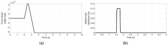
Figure 2. Test signals used for validation. (a) A fish-hook maneuver applied on the front wheel [35]. (b) An exogenous vertical road reference pulse to simulate a speed bump.

Figure 3 shows comparatives of the state variables (angles); such variables are calculated employing the model and compared with against those provided by CarSim. The vehicle speed is initialized to 22 m/s and left open throttle (no braking/accelerating torque in the wheels, only rolling resistance is stopping the TWV). The dynamic behavior of the model presents in average minimal error; this validation allows to show that the model is adequate for a control design in such operating point. Parameters as the stiffness-coefficients of the tires and suspension are tuned for such maneuver and are shown in Table 2. For the pitch angle validation, a 100 N braking force in the front wheel is entered, otherwise, the pitch angle is almost constant along with the maneuver.

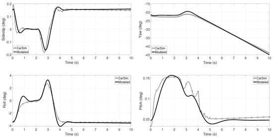
Figure 3. Comparison of the TWV side slip and Euler’s angles, calculated by means of the presented model and those provided by CarSim. In average, the error is minimal and as expected; the model can not reproduce a highly non-linear behavior as small oscillations, for instance.

The risk indexes are validated by comparison with those obtained from CarSim by direct calculation from its definitions (Equations (11), (16) and (18)); this software provides the longitudinal, lateral and vertical forces on the wheels. Since CarSim does not provide the angular accelerations for roll and pitch, these are calculated in Simulink; regardless of the above, the calculation of the risk indexes can be done in a real application by using an IMU and proper signal conditioning.

In order to validate the risk of rollover in the direction of the roll angle, the fish-hook maneuver of Figure 2a is used but increased in steps of 100 up to $400\%$. In Figure 4 comparatives of the $R{I}_{\phi }$ for such maneuvers are shown. Again, although the model cannot reproduce rapid oscillations (caused by the soft suspension of the TWV), it is sufficient to predict if there is a risk of rollover in the direction of $\phi$. With the maneuver increased by $300\%$, there is a loss of vertical force in a rear wheel, and the risk index is one or more (absolute value) in such intervals. With the maneuver increased by $400\%$, there is a lift of the right rear wheel and the vehicle ends up completely overturning.

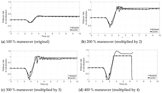
Figure 4. Comparison of the rollover risk in roll direction ($R{I}_{\phi }$) modeled in this paper, and calculated by the vertical forces provided by CarSim, using the maneuver of Figure 2a multiplied by 100, 200, 300, and $400\%$. The model presented in this paper is precise enough to detect an imminent rollover to the left or right side. With the $400\%$ maneuver, the TWV rollovers to the left; from second 3.65 onwards, the rear right wheel is lifted off the ground.

The rollover index risk in the direction of the pitch angle is validated by the introduction (adding) of a vertical road reference pulse (simulating a speed bump); if it is of sufficient height, this lifts the front wheel. The pulse of Figure 2b is used, with increments of $100\%$ up to $400\%$. Figure 5 shows comparatives of the modeled rollover risk in the pitch direction against the calculation of Equation (16). With the pulse augmented by $400\%$, the front wheel tipping is obvious at second $1.78$.

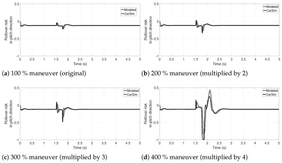
Figure 5. Comparison of the rollover risk in pitch direction ($R{I}_{\mathcal{X}}$) modeled in this paper, and calculated by the vertical forces provided by CarSim, using the front vertical road reference pulse of Figure 2b multiplied by 100, 200, 300 and $400\%$. The model presented in this paper is enough precise to detect an imminent longitudinal rollover; with the $400\%$ impulse, the front wheel is lifted off the ground.

In order to validate the skid risk index, the friction coefficient is set to $\mu =0.5$ and a 150 N rear accelerating force on each rear wheel is applied. With such a parameter combination is extremely easy to induce a tripped rollover; that is, the vehicle skids until it rollovers. The fish-hook maneuver of Figure 2a is used again, augmented by steps as in the previous cases. In Figure 6 the skid index comparisons are shown. For the $100\%$ maneuver exclusively, the TWV can follow the fish-hook maneuver without a tripped rollover neither a skid. In this case, the modeled $SI$ shows a more conservative estimate of the risk; also, once a wheel of the TWV has been lifted, the estimation is erratic. This is because a mitigation system must interact to avoid the $SI$ reaching absolute values near one.

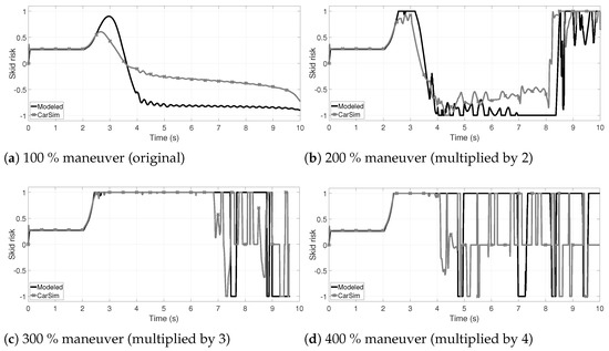
Figure 6. Comparison of the skid risk ($SI$) modeled in this paper, and calculated by the vertical forces provided by CarSim, using the maneuver of Figure 2a multiplied by 100, 200, 300 and $400\%$. Rear tracking force (accelerating on both wheels) of 150 N, with $\mu =0.5$ are used to induce the skid with aggressive maneuvers. The model presented in this paper is enough precise to detect an imminent skid. Only the $100\%$ maneuver can be performed without a skid; even with the $200\%$ maneuver, the TWV skids and eventually suffers a tripped rollover (skid and roll).

It is worth mentioning that the combination of a low coefficient of friction with speed bumps, potholes and/or other vertical exogenous forces during a maneuver, such as the fish-hook one (a combination of high risks’ levels, shown in later sections), considerably increases the risk of an accident.

It is worth mentioning that all taken considerations for the modeling result in a conservative estimation of the risks, as shown in the previous figures. Hence, although the presented models are not suitable for an accurate description of the TWV dynamics over all possible conditions and scenarios, it is enough and tractable for the design of a DSC following a conservative objective of mitigating the risks.

3. Robust Mitigation System Design

From equations for risk indexes (11), (16) and (18), a state-feedback of the state-variables $\dot{\psi }$, $\phi$, $\dot{\phi }$, and $\dot{\mathcal{X}}$ is suitable to diminish the risk indexes. The pitch angle ($\mathcal{X}$) must not be included since it is not desirable to correct the longitudinal unbalance of the $CoG$ (rarely the $CoG$ is longitudinally centered in a real a TWV). Even more, such state variables are easily obtained by an IMU and the calculation of the risk indexes is not necessary for feedback (only during the design).

In order to generate a counter torque in the direction of the yaw angle (contrary to the curve), it is proposed that one rear wheel brake and the other accelerate, with a force magnitude as close to equal as possible. Also, in this way, the risk of skidding will not be increased because the terms $F_{LRL}$, $F_{LRR}$ are almost canceled out in Equation (19). Also, for a rollover risk in the pitch direction, all-wheel braking/accelerating with an equitable distribution on front/rear wheels is proposed, to contribute to the differential braking/accelerating control law.

The proposed control law ($F_{LRL}$, $F_{LRR}$ and $F_{LF}$) for the system of Equation (10) is then:

$$\begin{array}{c}\hfill U=Ky=\left[\begin{array}{cccccc}0& 0& 0& 0& k_1& 0\\ 0& k_2& k_3& k_4& -0.5k_1& 0\\ 0& -k_2& -k_3& -k_4& -0.5k_1& 0\end{array}\right]\left[\begin{array}{c}\beta \\ \dot{\psi }\\ \dot{\phi }\\ \phi \\ \dot{\mathcal{X}}\\ \mathcal{X}\end{array}\right]\end{array}$$

(21)

In order to find suitable values for the control gains matrix K under arbitrary but bounded parameter-varying, first the closed-loop system is coordinate-transformed (the stability property of a system is preserved for an operating point shifting). Later, a polytopic representation is obtained, whose vertexes are calculated with the bounds for the K entries and a global parameter variation conservatively proposed as a scaling factor; LMI software allows one to numerically determine the bounds of the K entries for a common Lyapunov function. Subsequently, the best K entries are obtained by an optimization algorithm.

The closed-loop system turns on:

$$\begin{array}{c}\hfill \dot{y}=Ay+C\end{array}$$

(22)

where

$$\overline{A}=\left[\begin{array}{cccccc}-\frac{c_f+c_r}{mv}& \frac{c_r{l}_r-c_f{l}_f-m{v}^2}{m{v}^2}& 0& 0& \frac{\delta k_1}{mv}& 0\\ \frac{c_r{l}_r-c_f{l}_f}{J}& \frac{b{k}_{2}v-c_f{l}_f^2+c_r{l}_r^2}{Jv}& \frac{b{k}_3}{J}& \frac{b{k}_4}{J}& \frac{0.5k_1(b_l-b_r)+\delta k_1{l}_f}{J}& 0\\ -\frac{h(c_f+c_r)}{J_{\phi }}& \frac{h(c_r{l}_r-c_f{l}_f)}{v{J}_{\phi }}& -\frac{c_{\phi }}{J_{\phi }}& \frac{mgh-k_{\phi }}{J_{\phi }}& \frac{\delta k_{1}h}{J_{\phi }}& 0\\ 0& 0& 1& 0& 0& 0\\ \frac{h{c}_f\delta }{J_{\mathcal{X}}}& \frac{h{c}_f{l}_f\delta }{v{J}_{\mathcal{X}}}& 0& 0& \frac{h{k}_1-c_{\mathcal{X}}+2h0.5k_1}{J_{\mathcal{X}}}& \frac{mgh-k_{\mathcal{X}}}{J_{\mathcal{X}}}\\ 0& 0& 0& 0& 1& 0\end{array}\right]$$

Consider the linear variable change $x=y+A^{-1}C$ with $x={[x_1,x_2,x_3,x_4,x_5,x_6]}^{\prime }$ (see [36] (p. 112)); then the dynamic system (22) turns in:

$$\begin{array}{ccc}\hfill \dot{x}& =& Ax\hfill \end{array}$$

(23)

In order to establish robust stability for the closed-loop system (23) against model and parameter uncertainty, a polytopic representation is defined and a common Lyapunov function is foreseen to ensure stability despite arbitrary-rate varying-parameters. Consider a bounded parameter variation as follows:

$$\begin{array}{ccc}\hfill \dot{x}& =& \theta Ax\hfill \end{array}$$

(24)

where $0<{\theta }_m\le \theta \le {\theta }_M$ is a real number. For instance, $0.9\le \theta \le 1.1$ represents a $\pm 10\%$ global variation of parameters. Note that this is a more conservative definition of uncertainty than those defined by independently varying entries of A; the vertexes can be obtained for a particular set of uncertain parameters while the following analysis is still valid. Hence, two vertexes are obtained, ${\theta }_{m}A$ and ${\theta }_{M}A$, where $\delta =\parallel {\delta }_M\parallel$ (a maximum steering angle) is used.

Under regular parameter values (generally $c_R>c_F$, $k_{\phi }>mgh$, $k_{\mathcal{X}}>mgh$), the vertexes meets the Sylvester’s criterion for negative definite matrices if:

$$\begin{array}{c}\hfill k_1\le 0\\ \hfill k_2\le 0\\ \hfill k_3\le 0\\ \hfill k_4\le 0\end{array}$$

(25)

ensuring the stability of each vertex. However as [37] (p. 2) confirms, is not enough to ensure the stability of each vertex, to ensure the global stability of the linear time-variant system (24). Instead, a common Lyapunov function ensures the global stability under arbitrary (abrupt but bounded) parameter varying, and even under arbitrary switching between vertexes. To this end, upper bounds on $k_1,...,k_4$ are established (they are numerically unknown yet), then

$$\begin{array}{c}\hfill k_{1,m}\le k_1\le 0\\ \hfill k_{2,m}\le k_2\le 0\\ \hfill k_{3,m}\le k_3\le 0\\ \hfill k_{4,m}\le k_4\le 0\end{array}$$

(26)

increasing the number of vertexes to $2^5$:

• ${\theta }_{m}A$ calculated with $k_1=k_{1,m}$, $k_2=k_{2,m}$, $k_3=k_{3,m}$ and $k_4=k_{4,m}$ named $A_1$,
• ${\theta }_{m}A$ calculated with $k_1=k_{1,m}$, $k_2=k_{2,m}$, $k_3=k_{3,m}$ and $k_4=0$ named $A_2$,
• ${\theta }_{m}A$ calculated with $k_1=k_{1,m}$, $k_2=k_{2,m}$, $k_3=0$ and $k_4=k_{4,m}$ named $A_3$,
• ${\theta }_{m}A$ calculated with $k_1=k_{1,m}$, $k_2=k_{2,m}$, $k_3=0$ and $k_4=0$ named $A_4$,
• ...
• ${\theta }_{M}A$ calculated with $k_1=0$, $k_2=0$, $k_3=0$ and $k_4=k_{4,m}$ named $A_{31}$.
• ${\theta }_{M}A$ calculated with $k_1=0$, $k_2=0$, $k_3=0$ and $k_4=0$ named $A_{32}$.

Therefore, the system (24) turns into the polytopic system:

$$\begin{array}{ccc}\hfill \dot{x}& =& A_{i}x,\forall i\in \{1,2,...,32\}.\hfill \end{array}$$

(27)

A common Lyapunov candidate function is $V=x^{\prime }Px$, such that one looks to find a positive definite matrix P ([38] (p. 9)) such that:

$$\begin{array}{c}\hfill P{A}_i+A_i^{\prime }P\preccurlyeq 0,\forall i\in \{1,2,...,32\}.\end{array}$$

(28)

Therefore, $P{A}_i+A_i^{\prime }P$ must be negative definite matrices. The determination of P can be carried out numerically, for example, using the MATLAB library called YALMIP [39]. Its existence depends on the parameters, and the ${\theta }_m,{\theta }_M$ and $k_1,...,k_4$ values. In the following, an algorithm (Algorithm 1) is presented to numerically find appropriate values for P, ${\theta }_m,{\theta }_M$, $k_1,...,k_4$, and $k_{1,m},...,k_{4,m}$.

Algorithm 1 An algorithm is presented to numerically find appropriate values for P, ${\theta }_m,{\theta }_M$, $k_1,...,k_4$, and $k_{1,m},...,k_{4,m}$.

Initialize ${\theta }_m={\theta }_M=1$ and $k_h=k_{h,m}=0$, $\forall h\in 1,2,3,4$. Try to solve the LMI, $P{A}_i+A_i^{\prime }P\preccurlyeq 0$. If P cannot be found, verify the used parameters. Increase ${\theta }_M$ and decrease ${\theta }_m$ by small steps and try to solve the LMI, $P{A}_i+A_i^{\prime }P\preccurlyeq 0$. Repeat the Step 3 if P is found. If P cannot be found anymore, fix the smaller and largest ${\theta }_m,{\theta }_M$ values for which the LMI has a solution. If $k_{1,m}\ne 0$ go to Step 9. Decrease $k_1$ by a small step $k_{1,\Delta }$ and try to solve the LMI, $P{A}_i+A_i^{\prime }P\preccurlyeq 0$. If P cannot be found, set $k_{1,m}=k_1+k_{1,\Delta }$. If $k_{2,m}\ne 0$ go to Step 12. Decrease $k_2$ by a small step $k_{2,\Delta }$ and try to solve the LMI, $P{A}_i+A_i^{\prime }P\preccurlyeq 0$. If P cannot be found, set $k_{2,m}=k_2+k_{2,\Delta }$. If $k_{3,m}\ne 0$ go to Step 15. Decrease $k_3$ by a small step $k_{3,\Delta }$ and try to solve the LMI, $P{A}_i+A_i^{\prime }P\preccurlyeq 0$. If P cannot be found, set $k_{3,m}=k_3+k_{3,\Delta }$. If $k_{4,m}\ne 0$ go to Step 18. Decrease $k_4$ by a small step $k_{4,\Delta }$ and try to solve the LMI, $P{A}_i+A_i^{\prime }P\preccurlyeq 0$. If P cannot be found, set $k_{4,m}=k_4+k_{4,\Delta }$. If $k_{1,m}\ne 0$∧$k_{2,m}\ne 0$$k_{3,m}\ne 0$∧$k_{4,m}\ne 0$, then go to Step 20. Go to Step 6. Solve the following optimization problem, to find $k_1,...,k_4$ $$\begin{array}{ccc}\hfill \underset{k_1,...,k_4}{Minimize}& & \underset{0\le t\le T}{max}\left({∥R{I}_{\phi }∥}_2+{∥R{I}_{\mathcal{X}}∥}_2+{∥SI∥}_2\right)\hfill \\ \hfill Subjectto:& & \\ & & k_1\ge k_{1,m}\hfill \\ & & k_1\le 0\hfill \\ & & k_2\ge k_{2,m}\hfill \\ & & k_2\le 0\hfill \\ & & k_3\ge k_{3,m}\hfill \\ & & k_3\le 0\hfill \\ & & k_4\ge k_{4,m}\hfill \\ & & k_4\le 0\hfill \\ & & \dot{y}=(A+BK)y+C\hfill \end{array}$$ where T is a time horizon. End

In Algorithm 1, one looks to find the first bounds for the parametric variation. Then, bounds for the controller gains are found, and finally, one looks for the combination of gains (within the bounds for stability) that the best results provide for minimizing the risks. In Section 4, the resolution of the Algorithm 1 for the parameters of Table 1 is exemplified. Also, note that exogenous perturbations can be added during Step 20 to emulate a driving with speed bumps for instance.

Resolution of the Algorithm 1, ensures the robust stability of the system for any parametric variation within the bounds, provides bounds for the controller gains and ensures the best performance (tuning) of the controller on minimizing the risk.

Although another criterion other than the squared maximum risk could have been selected on Step 20, such as the mean square error or the standard deviation, this was chosen for its fast calculation; as well, the result is in practical terms the same. In Section 4, the resolution of Algorithm 1 for the parameters of Table 2 is exemplified; both criteria, the mean square error and standard-deviation, are included in such exemplification.

4. Performance Evaluation of the DSC

4.1. Controller Numerical Design

Consider the parameters of Table 2. With $T=7$ s, steps of $0.1$ for the parametric variation, unitary steps for gains and $\delta =0.45$ rad. The Algorithm 1 results on a $\pm 20.2\%$ variation (${\theta }_m=0.798$, ${\theta }_M=1.202$), $k_1=-47388$, $k_2=-11007$, $k_3=-221$, $k_4=-1000$ with a squared risk of $0.154629$ units and:

$$\begin{array}{ccc}\hfill P& =& 1\times {10}^4\left[\begin{array}{cccccc}3.6238& 0.2413& -0.0133& 0.1927& -0.0069& 0.0333\\ 0.2413& 0.1270& -0.0036& 0.0012& -0.0018& 0.0004\\ -0.0133& -0.0036& 0.0014& 0.0002& 0.0000& 0.0000\\ 0.1927& 0.0012& 0.0002& 0.0870& -0.0002& 0.0005\\ -0.0069& -0.0018& 0.0000& -0.0002& 0.2472& 0.1469\\ 0.0333& 0.0004& 0.0000& 0.0005& 0.1469& 4.6418\end{array}\right].\hfill \end{array}$$

The LMI problem (28) for this example is solved in MATLAB by the recursive use of the YALMIP library [39] with SeDuMi solver [40].

For completeness purposes, mean squared error and standard deviation ($\sigma$) are also used for Algorithm 1 resolution; mean-squared error is $0.0046810402$ and $\sigma =0.026073196$ for the best tuning. In Figure 7 are shown comparatively the maximum (peak) ${∥R{I}_{\phi }∥}_2+{∥R{I}_{\mathcal{X}}∥}_2+{∥SI∥}_2$ for the numerical integration of the model, against the mean-squared error and standard deviation. As can be seen, the results are comparable but calculating the squared maximum/peak is faster than other criteria (some large operations are avoided).

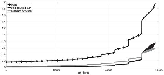
Figure 7. Comparison of different objective functions used in the algorithm. Results for each $k_i$ combinations are ordered by peak-risk; the mean-squared error and standard deviation follows the same tendency. The squared peak/maximum criterion is of faster calculation and throws, in practical terms, the same results. Only 10 steps of each $k_i$ range are plotted.

4.2. Real-Time HIL Experiments

In order to evaluate the behavior of the DSC, hardware in the loop (HIL) tests are performed. The vehicle is emulated in CarSim on a PC (Intel I7 with 16 GB RAM), while RS232 communication allows an external device to read and calculate the braking/accelerating forces (Figure 8). Since the used version of CarSim does not allow RS232 communication but can interact with Simulink (MATLAB), this last is used as a communication interface with the DSC. The external device (DSC prototype) consists of a DSPIC33 from Microchip digital signal processor that includes CAN-Bus communications. However, a RS232 bidirectional communication is used since the PC does not have integrated CAN-Bus. The printed circuit board of the DSC prototype is also shown in Figure 8. The DSC is supposed to read an inertial measurement unit for Euler angles and their speeds and accelerations in a real scenario; for this HIL test, CarSim is programmed to send these signals to the DSC. In a real scenario, additional signals can be read/written from the vehicle’s PCM via CAN-Bus communications. The output signals emitted by the DSC for this HIL test are the longitudinal forces in each wheel; in a real scenario, these will be replaced by signals to the vehicle’s ABS module and to the PCM itself with braking and acceleration commands on each wheel.

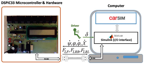
Figure 8. HIL test platform and printed circuit board of the DSC. The vehicle is emulated in CarSim on a PC (Intel I7 with 16 GB RAM); Simulink serves as a communication interface with the external DSC. The DSC prototype includes a DSPIC33F DSP, LCD display, 8 CAN/ECAN-Bus ports and a serial port with their respective interfaces. The DSP operates at 60 MIPS and the RS232 is programmed to operate at 56 kbps.

For this first set of semi-experimental tests, the maneuver of Figure 2a augmented by $300\%$ is used, in addition to the exogenous road reference step of Figure 2b applied on front-wheel but beginning at $5.6$ s, and the same exogenous pulse applied $0.1$ seconds later on the rear wheel (in order to emulate a speed bump during the curve). Also, the parameters of Table 2 are used with exception of the friction coefficient; $\mu =0.45$, $\mu =0.65$ and $\mu =0.85$ are used instead, in order to evaluate the DSC dynamical behavior on $\phi$, $\mathcal{X}$, $\psi$, as well as the displacement over the inertial frame and the risk indexes.

In Figure 9, Figure 10 and Figure 11 the comparative results of the roll, pitch and yaw angles, as well as the displacement of the $CoG$ over the $X_{IN}-Y_{IN}$-plane in the $\mu =0.45$, $\mu =0.65$ and $\mu =0.85$ scenarios are shown. Star marked plots correspond to open-loop dynamics. In the three open-loop scenarios, the vehicle rollovers once the speed-bump is passed by, as the roll angle indicates. From Figure 4a it is apparent that this maneuver did not involve a rollover with $\mu =0.75$ and without the speed bump. In closed-loop, the rollover is avoided regardless the variation in the friction coefficient; it is worth to mention that in fact, inevitably the 3 tires of the vehicle loose ground contact at second $5.8$ but, in closed-loop, the driveability is restored. It is important to note that, at low $\mu$ the rollover occurs faster than at $\mu =0.85$ in open-loop. In the Supplementary Material Section, a link is provided to video animations of these HIL tests.

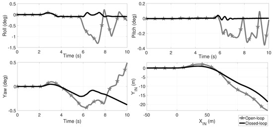
Figure 9. Comparative of the roll, pitch and yaw angles as well as the TWV displacement for open (black plots) and closed-loop (gray-star marked plots), and a friction coefficient $\mu =0.45$ for the maneuver of Figure 2a augmented by $300\%$. At the second $5.6$, a speed bump is simulated by an exogenous road step (Figure 2b) in the front wheel and $0.1$ seconds later in the rear right wheel. In open-loop, the vehicle suffers a rollover from second 6 as the roll angle indicates and in closed-loop the rollover is avoided; since the three wheels lose ground contact at second $5.8$ oscillations are expected at the TWV landing. In the Supplementary Material Section, a link is provided with video animations.

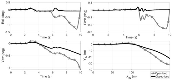
Figure 10. Comparative of the roll, pitch and yaw angles as well as the TWV displacement for open (black plots) and closed-loop (gray-star marked plots), and a friction coefficient $\mu =0.65$ for the maneuver of Figure 2a augmented by $300\%$. At the second $5.6$, a speed bump is simulated by an exogenous road step (Figure 2b) in the front wheel and $0.1$ seconds later in the rear right wheel. In open-loop, the vehicle suffers a rollover from second 6 as the roll angle indicates and in closed-loop the rollover is avoided; since the three wheels lose ground contact at second $5.8$ oscillations are expected at TWV landing. In the Supplementary Material Section, a link is provided to video animations.

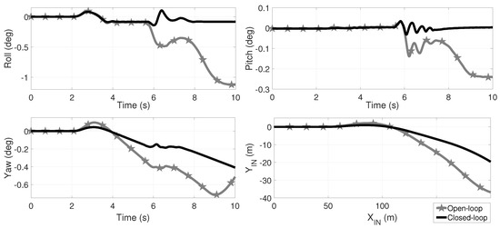
Figure 11. Comparative of the roll, pitch and yaw angles as well as the TWV displacement for open (black plots) and closed-loop (gray-star marked plots), and a friction coefficient $\mu =0.85$ for the maneuver of Figure 2a augmented by $300\%$. At the second $5.6$, a speed bump is simulated by an exogenous road step (Figure 2b) in the front wheel and $0.1$ seconds later in the rear right wheel. In open-loop, the vehicle suffers a rollover from second 6 as the roll angle indicates and in closed-loop the rollover is avoided; since the three wheels lose ground contact at second $5.8$ oscillations are expected at TWV landing. In the Supplementary Material Section, a link is provided to video animations.

Now, consider the parameters of Table 2 with the following changes: $\mu =0.6$, $l_f=0.882$ m, $l_r=1.143$ m, $h=0.432$ m, $b_r=0.625$ m, $bl=0.425$ m and $m=597$ kg. In Figure 12 is shown the comparative for roll, pitch and yaw angles, as well as the TWV’s $CoG$ displacement. Despite the parameter variation, the augmented maneuver by $300\%$ and the road pulse simulating a speed bump, in closed-loop the rollover is mitigated while in open-loop the TWV suffers a rollover. In the Supplementary Material Section, a link is provided to video animations of these HIL tests.

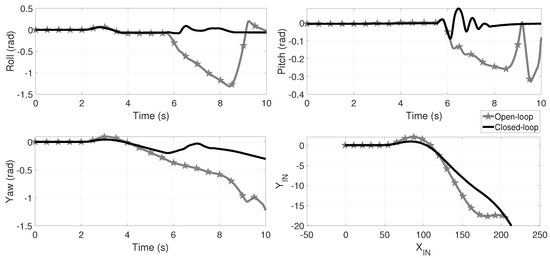
Figure 12. Comparative of the roll, pitch and yaw angles as well as the TWV displacement for open (black plots) and closed-loop (gray, star marked plots) for the maneuver of Figure 2a augmented by $300\%$. Also, $\mu =0.6$$l_f=0.882$ m, $l_r=1.143$ m, $h=0.432$ m, $b_r=0.625$ m, $bl=0.425$ m and $m=597$ kg. At second $5.6$, a speed bump is simulated by an exogenous road step (Figure 2b) in the front wheel and $0.1$ seconds later in the rear right wheel. In open-loop the vehicle suffers a rollover from second 6 as the roll angle indicates and in closed-loop the rollover is avoided despite the parametric variation; since the three wheel loose ground contact at second $5.8$ oscillations are expected at TWV landing. In the Supplementary Material Section, a link is provided to video animations.

Finally, in Figure 13 is shown a comparative of the roll angles for open and closed-loop, illustrating that if the rear left wheel passes by a pothole, ($-0.15$ m) for the maneuver of Figure 2a augmented by $300\%$, a tripped rollover occurs. In this tests, $\mu =0.6$ (to induce the skidding), $l_f=0.882$ m, $l_r=1.143$ m, $h=0.432$ m, $b_r=0.625$ m, $bl=0.425$ m and $m=597$ kg. In open-loop the vehicle suffers a rollover with the pothole and a skid without the pothole. In closed-loop the rollover is mitigated despite the wheels lifting. See Figure 14 for a pictorial illustration; other pictorial illustrations and different scenarios are not included here but, indeed, the DSC can mitigate a wide variety of accidents. In the Supplementary Material Section, a link is provided to video animations of these HIL tests.

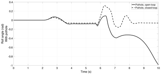
Figure 13. Comparative of the roll angle for open and closed-loop, with a pothole in the rear left wheel ($-0.15$ at $5.6$ s), for the maneuver of Figure 2a augmented by $300\%$. Also, $\mu =0.6$, $l_f=0.882$ m, $l_r=1.143$ m, $h=0.432$ m, $b_r=0.625$ m, $bl=0.425$ m and $m=597$ kg. In open-loop the vehicle suffers a rollover with the pothole. In closed-loop the rollover is mitigated despite wheels lifting. See Figure 14 for a pictorial illustration. In the Supplementary Material Section, a link is provided to video animations.

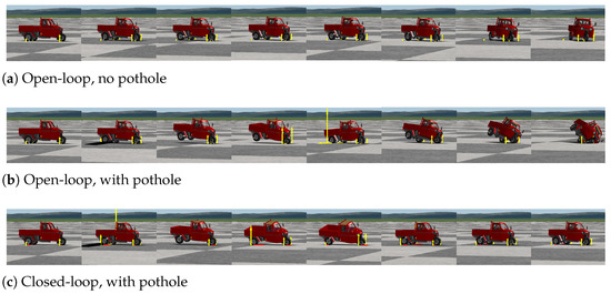
Figure 14. Comparative of TWV animations in open (up and middle) and closed-loop (bottom) with $\mu =0.6$, $l_f=0.882$ m, $l_r=1.143$ m, $h=0.432$ m, $b_r=0.625$ m, $bl=0.425$ m and $m=597$ kg, for the maneuver of Figure 2a augmented by $300\%$. The pothole is simulated for the last two simulations by the exogenous road step of Figure 2b multiplied by $-1$ and shifted to begin at second $5.6$, only in the rear left wheel. Snapshots are taken at the same distance from the beginning of the maneuver. The DSC can recover the driveability of the TWV and avoid the rollover. In the Supplementary Material Section, a link is provided to the full video.

5. Conclusions

In this paper, it is shown that the in-wheel motor torques of a delta three-wheeled vehicle can be used to design an active safety system to assist the driver and mitigate tripped and un-tripped rollovers (within the limits of physics). The designed differential braking/accelerating controller can mitigate rollovers even if the vehicle passes a pothole or a speed bump during a curve. Also, the controller can mitigate the risk of skidding regardless of whether it could cause a rollover or not. Implementation of the controller is simple on a TWV and requires a cheap DSP with some peripherals and the measuring of chassis angular variables. The braking/accelerating commands can be sent to the main vehicle’s computer and the ABS braking module via CAN-Bus communications. The DSC can help to mitigate both side and longitudinal rollovers (tripped and un-tripped), even after the vehicle has lost (and recovers) tire-ground contact. It is worth mentioning that the DSC, like any active vehicle safety system, is an assistance system and will not be able to prevent every rollover in every scenario. However, it is shown that it does provide assistance and mitigation in various scenarios, despite variation in load and changes in the position of the center of gravity. Future work consists of integrating the actuator dynamics and develop a real implementation.

References

- Zandieh, A. Dynamics of a Three_Wheel Vehicle with Tadpole Design. Master’s Thesis, University of Waterloo, Waterloo, ON, Canada, 2015. [Google Scholar]
- Kumar, N.; Katiyar, G. Tadpole Configuration for Three-Wheeled Vehicles; SAE Technical Paper; SAE International: Warrendale, PA, USA, 2020. [Google Scholar]
- Gawade, T.; Mukherjee, S.; Mohan, D. Rollover Propensity of Three-Wheel Scooter Taxis. SAE Technical Paper. SAE International: Warrendale, PA, USA, 2004. [Google Scholar]
- Mukherjee, S.; Mohan, D.; Gawade, T.R. Three-wheeled scooter taxi: A safety analysis. Sadhana 2007, 32, 459–478. [Google Scholar] [CrossRef][Green Version]
- Phanomchoeng, G.; Rajamani, R. New rollover index for the detection of tripped and untripped rollovers. IEEE Trans. Ind. Electron. 2012, 60, 4726–4736. [Google Scholar] [CrossRef]
- Hailu, M.G.; Thakur, A.; Leake, O. Reverse engineering approach in modification of three wheeler Bajaj chassis. Branna J. Eng. Technol. 2020, 2, 21–40. [Google Scholar]
- Spânu, A.; Stoenescu, F.; Lorenzi, M.; Avram, M. Analysis of three wheeled electric vehicle with increased stability on the road. MS&E 2018, 444, 042010. [Google Scholar]
- Okpala, C.C.; Chukwuzitelu, J.C.; Okeke, P.O.; Egwu, S.I. Design and fabrication of an optimized low cost cargo-bearing tricycle. Int. J. Adv. Eng. Technol. 2017, 3, 9. [Google Scholar]
- Mulla, T.M.; Kadam, S.J.; Kengar, V.S. Finite element analysis of helical coil compression spring for three wheeler automotive front suspension. Int. J. Mech. Ind. Eng. 2012, 2, 74–77. [Google Scholar]
- Ram, S.A.S.; Raja, P.; Sreedaran, K. Optimization of rollover stability for a three-wheeler vehicle. Adv. Manuf. 2017, 5, 279–288. [Google Scholar]
- Van Valkenburgh, P.G.; Klein, R.H.; Kanianthra, J. Three-wheel passenger vehicle stability and handling. SAE Trans. 1982, 91, 605–627. [Google Scholar]
- Azim, R.A.; Malik, F.M. Rollover mitigation controller development for three-wheeled vehicle using active front steering. Math. Probl. Eng. 2015, 2015, 1–10. [Google Scholar] [CrossRef]
- Sindha, J.; Chakraborty, B.; Chakravarty, D. Automatic stability control of three-wheeler vehicles—Recent developments and concerns towards a sustainable technology. Proc. Inst. Mech. Eng. Part D J. Automob. Eng. 2018, 232, 418–434. [Google Scholar] [CrossRef]
- Ojolo, S.J.; Ajayi, O.O.; Asuelinmen, G.A. Rollover stability models for three-wheeled vehicle design. Arid. Zone J. Eng. Technol. Environ. 2020, 16, 92–99. [Google Scholar]
- Asuelinmen, G.A.; Ojolo, S.J.; Ajayi, O.O. Investigating the lateral stability of three-wheeled scooter taxi due to tyre-road forces. Niger. J. Technol. 2020, 39, 189–195. [Google Scholar] [CrossRef]
- Azim, R.A. Rollover Mitigation Controller Development for a Three Wheeled Platform. Ph.D. Thesis, National University of Sciences and Technology, Islamabad, Pakistan, 2015. [Google Scholar]
- Saeedi, M.A.; Kazemi, R. Stability of three-wheeled vehicles with and without control system. Int. J. Automot. Eng. 2013, 3, 343–355. [Google Scholar]
- Ataei, M.; Khajepour, A.; Jeon, S. Reconfigurable integrated stability control for four-and three-wheeled urban vehicles with flexible combinations of actuation systems. IEEE/ASME Trans. Mechatron. 2018, 23, 2031–2041. [Google Scholar] [CrossRef]
- Khanna, N.; Arora, A. Methodology and Experimental Study to Reduce Steering Effort and Improve Directional Stability in a Three Wheeled Vehicle; SAE Technical Paper; SAE International: Warrendale, PA, USA, 2020. [Google Scholar]
- Waseem, M.; Suhaib, M.; Sherwani, A.F. Modelling and analysis of gradient effect on the dynamic performance of three-wheeled vehicle system using Simscape. SN Appl. Sci. 2019, 1, 225. [Google Scholar] [CrossRef]
- Ataei, M.; Khajepour, A.; Jeon, S. Rollover stabilities of three-wheeled vehicles including road configuration effects. Proc. Inst. Mech. Eng. Part D J. Automob. Eng. 2017, 231, 859–871. [Google Scholar] [CrossRef]
- Alfiany, N.; Hamid, N.; Jati, G.; Ma’sum, M.A.; Jatmiko, W. Kinematics and dynamics analysis of an autonomous dhree-wheeled bicycle modeling. In Proceedings of the 2019 4th Asia-Pacific Conference on Intelligent Robot Systems (ACIRS), Nagoya, Japan, 13–15 July 2019; IEEE: Piscataway, NJ, USA, 2019; pp. 17–21. [Google Scholar]
- Pandey, A.; Jha, S.; Chakravarty, D. Modeling and control of an autonomous three wheeled mobile robot with front steer. In Proceedings of the 2017 First IEEE International Conference on Robotic Computing (IRC), Taichung, Taiwan, 10–12 April 2017; IEEE: Piscataway, NJ, USA, 2017; pp. 136–142. [Google Scholar]
- Margetts, R. Modelling the dynamics of a three-wheeled racecar: A pilot study to establish the feasibility of developing a ‘delta’ configuration performance car. Preprints 2018. Available online: https://www.mdpi.com/ethics (accessed on 10 July 2021).
- Karanam, V.M.; Ghosal, A. Studies on the wobble mode stability of a three-wheeled vehicle. Proc. Inst. Mech. Eng. Part D J. Automob. Eng. 2013, 227, 1200–1209. [Google Scholar] [CrossRef]
- Dizo, J.; Blatnicky, M. Evaluation of vibrational properties of a three-wheeled vehicle in terms of comfort. Manuf. Technol. 2019, 19, 197–203. [Google Scholar] [CrossRef]
- Behera, A.; Sivalingam, M. Experimental and simulation studies on instability of a two wheeler vehicle. SAE Int. J. Veh. Dyn. Stab. NVH 2017, 1, 234–246. [Google Scholar] [CrossRef]
- Grzegożek, W.; Zagól, B.; Kot, A. Analysis of lean angle influence on three wheeled vehicle steerability characteristics. In International Scientific Conference Transport of the 21st Century; Springer: Berlin, Germany, 2019; pp. 164–172. [Google Scholar]
- Dižo, J.; Blatnickỳ, M.; Kurčík, P. Analysis of driving properties of a three-wheeled vehicle with a newly designed steering system. In MATEC Web of Conferences; EDP Sciences: Les Ulis, France, 2019; Volume 254, p. 03008. [Google Scholar]
- Pacejka, H. Tire and Vehicle Dynamics; Elsevier: Amsterdam, The Netherlands, 2005. [Google Scholar]
- Gawade, T.R.; Mukherjee, S.; Mohan, D. Six-degree-of-freedom three-wheeled-vehicle model validation. Proc. Inst. Mech. Eng. Part D J. Automob. Eng. 2005, 219, 487–498. [Google Scholar] [CrossRef]
- Kiencke, U.; Nielsen, L. Automotive Control Systems: For Engine, Driveline, and Vehicle; IOP Publishing: Bristol, UK, 2000. [Google Scholar]
- Pearson, J. Vehicle Weights and Dimension Limits within the Nafta Partnership; Task Force on VW&D Policy: Ottawa, ON, Canada, 2002; 27p.
- Rodríguez-Licea, M.A.; Vazquez-Rodríguez, E.A.; Perez-Pinal, F.J.; Prado-Olivares, J. The rollover risk in delta tricycles: A new rollover index and its robust mitigation by rear differential braking. Math. Probl. Eng. 2018, 2018, 1–15. [Google Scholar] [CrossRef]
- Administration, N.H.T.S. Laboratory Test Procedure for Dynamic Rollover: The Fishhook Maneuver Test Procedure; US, Department of Transportation: Washington, DC, USA, 2013. [Google Scholar]
- Khalil, H.K.; Grizzle, J.W. Nonlinear Systems; Prentice Hall: Upper Saddle River, NJ, USA, 2002; Volume 3. [Google Scholar]
- Zhao, X.; Kao, Y.; Niu, B.; Wu, T. Control Synthesis of Switched Systems; Springer: Berlin, Germany, 2017. [Google Scholar]
- Boyd, S.; Laurent, E.G.; Feron, E.; Balakrishnan, V. Linear Matrix Inequalities in System and Control Theory; Siam: Philadelphia, PA, USA, 1994; Volume 15. [Google Scholar]
- Löfberg, J. YALMIP: A Toolbox for Modeling and Optimization in MATLAB. In Proceedings of the CACSD Conference, Taipei, Taiwan, 2–4 September 2004; pp. 284–289. [Google Scholar]
- Sturm, J.F. Using SeDuMi 1.02, a MATLAB toolbox for optimization over symmetric cones. Optim. Methods Softw. 1999, 11, 625–653. [Google Scholar] [CrossRef]
Publisher’s Note: MDPI stays neutral with regard to jurisdictional claims in published maps and institutional affiliations. |
© 2021 by the author. Licensee MDPI, Basel, Switzerland. This article is an open access article distributed under the terms and conditions of the Creative Commons Attribution (CC BY) license (https://creativecommons.org/licenses/by/4.0/).