Article

Dynamic Cosine Method for Normalizing Incidence Angle Effect on C-band Radar Backscattering Coefficient for Maize Canopies Based on NDVI

1
Northeast Institute of Geography and Agroecology, Chinese Academy of Sciences, Changchun 130102, China
2
College of Resources and Environment, University of Chinese Academy of Sciences, Beijing 100049, China
3
Changchun Jingyuetan Remote Sensing Test Site, Changchun 130102, China
4
School of Geomatics and Prospecting Engineering, Jilin Jianzhu University, Changchun 130118, China
5
College of Geoexploration Science and Technology, Jilin University, Changchun 130012, China
*
Author to whom correspondence should be addressed.
Remote Sens. 2021, 13(15), 2856; https://doi.org/10.3390/rs13152856
Submission received: 8 June 2021 / Revised: 15 July 2021 / Accepted: 19 July 2021 / Published: 21 July 2021

Abstract

:
Wide mode SAR images have an apparent incidence angle effect. The existing incident angle normalization methods assume that the relationship between the incident angle (θ) and the backscattering coefficient (σPQ) does not change with the growth stage of crops, which is in conflict with the real-life situation. Therefore, the normalization results of σPQ based on these existing methods will affect the accuracy of object classification, target recognition, and land surface parameter inversion. Here, the change in θ-σPQ relationship was investigated based on time-series (April to October) σPQ of maize canopies in northeast China, and a dynamic method based on normalized difference vegetation index (NDVI) was developed to normalize the effect of θ on σPQ. Through the accuracy evaluation, the following conclusions are obtained: (1) the dependence (referring to N) of Sentinel 1 C-band σPQ on θ varies with maize NDVI. In addition, the value of N changed from 9.35 to 0.66 at VV polarization from bare soil to biomass peak, and from 6.26 to 0.99 at VH polarization; (2) a dynamic method was proposed to quantify the change of N based on its strong correlation with NDVI, indicated by R2 of 0.82 and 0.80 for VV and VH polarization, respectively; and (3) the overall root mean square error of normalized σPQ based on the newly-developed dynamic method is 0.51 dB, and this accuracy outperforms the original first-order cosine method (1.37 dB) and cosine square law method (1.08 dB) by about 63% and 53% on the whole. This study provides a dynamic framework for normalizing radar backscatter coefficient, improving the retrieval accuracy of land surface parameters from radar remote sensing.

1. Introduction

SAR data are often used for land cover classification, target detection, and land surface parameter retrievals (leaf area index, snow water equivalent, and soil moisture) [1,2,3]. However, radar backscattering coefficient (σ0) changes with incident angle (θ) [4,5], show significant θ effect. For example, Radarsat σ0 of C-band Radarsat image changes 0.26 dB/° for a snow covered surface when θ ranges from 23° to 45° [6,7]. This incidence angle effect would reduce the accuracy of crop classification and soil moisture estimation based on change detection [8,9].
The dependence of σ0 on θ is related to polarization, land cover type, and crop growth stage [10,11,12]. At present, there are three methods for normalizing the radar incidence angle effect, including histogram matching method [13,14], linear method, and cosine method [15]. The histogram matching method is easy to apply, it only requires little prior knowledge, and its performance does not depend on sensor characteristics and ground conditions [10]. However, its normalized result may appear discontinuous in the range direction of the Radar image [11]. The linear method ignores the complex physical mechanism between σ0 and θ [16]. Furthermore, it requires a large number of auxiliary parameters and its normalized accuracy is higher in a specific study area, with poor portability [10]. The cosine model is derived from Lambert’s law [15], indicating the relationship between σ0 and θ obeys the law of cosine; it shows better performance for the homogeneous pixel.
The cosine method is one of the widely used normalization methods, first proposed by Clapp to eliminate the change of σ0 caused by θ [17]. It assumes that the amount of power reradiated in the upper hemisphere obeys the law of cosine [15]. Its formula is σ0 θ = σ0cosN(θ), σ0 is the backscattering coefficient independent of θ, and N is the power exponent of the cosine function, adjusting the dependence of σ0 on θ. The traditional cosine method adopts fixed N (N = 0, 1, 2), and this assumption cannot be well met for different ground features because the angle dependence of σ0 is affected by many factors.
Some studies have proven that radar parameters (polarization), land cover type, and crop growth stage are the important factors affecting the dependence of σ0 on θ [18,19,20], revealing the various N value in different cases. In terms of polarization, the N of non-irrigated olive trees is 6.3 and 5.5 for VV and HH polarization, respectively [21], and different N values are obtained for wetlands at different polarization modes (HH:2.4–2.5; VH:1.4–2.2; VV:2.1–2.8) [22]. In terms of land cover type, L-band ScanSAR image showed that the value of N for rainforest land cover types ranged from 0.24 to 3.36 [18], and another N value (N = 1.55) suitable for forest area is obtained [23]. The above results confirmed that the N value changes with forest types. The method considering the angle variation of σ0 for most land cover types was proposed, and successfully normalized the angle of vegetation communities in the Australian savanna landscape from radar images [24]. The angular dependence of ASAR WS backscatter is found to vary strongly over cropland [25]. Moreover, Lang et al. (2016) found that open water bodies and different types of ice affect the dependence of σ0 on θ [11]. In accordance with crop growth stage, the crop growth stage is seasonal in most cases [26], which leads to σ0 varying seasonally on the angle dependence. The dependence of σ0 on θ varies greatly in farmland, but little in permanent vegetation [25].
Summarizing the above results, it is found that a fixed N value is not suitable for changing land surface types, growth stages, and radar polarization modes. In agricultural areas, the dependence of σ0 on θ is mainly affected by crop types and crop growth stages. Aiming to reduce errors of normalized σ0, a NDVI (normalized difference vegetation index) representing the changes of crop growth stage, was used to quantify the angular sensitivity of radar signals [25]. The results show that NDVI has great potential in characterizing the angular sensitivity of C-band σ0 for wheat [27]. Although it has been recognized that the dependence of σ0 on θ is dynamic, the incidence angle normalization model of σ0 considering this dynamic change is rare. The biomass of maize is much larger than that of soybean and wheat in the whole growth stage, which has a great influence on radar signal scattering. This is helpful for us to study the influence of plant canopy on electromagnetic wave scattering from bare soil stage to maturity stage. To solve this problem, we plan to take maize as an example to investigate the relationship between σ0 and θ, and establish a general incidence angle normalization method of σ0 suitable for different crop growth stages, so as to improve the ability of radar data in ground object classification, target detection and land surface parameter retrievals.
This paper aims to investigate the variation characteristics of σ0 with respect to θ, and evaluates the angle normalization effect of cosine methods. In addition, a dynamic cosine model for incidence angle normalization of σ0 was proposed. This paper is composed of the following parts: Section 2 describes the study area, data sets and methods; Section 3 analyzes the relationship between σ0 and θ for maize and proposes and evaluates a new dynamic cosine method; Section 4 discusses the advantages and disadvantages of the newly proposed method; and Section 5 provides the conclusion.

2. Data and Methods

2.1. Study Site and Data Sets

2.1.1. Study Areas

The study site is located in the central part of Jilin Province in northeast China (123°08′~127°09′ E, 43°10′~44°51′ N) with an area of approximately 250 km×160 km, covering Changchun, Songyuan, Siping, and Jilin city (Figure 1). It belongs to the hinterland of the Songliao Plain in northeast China. It is one of the most important commercial maize production bases in China, and one of the three major black soil regions as well as three golden maize belts in the world [28]. Maize is the main crop in the study area, and the maize planting area accounts for 74.8% of the total crop area. The study area has a temperate continental monsoon climate, with four distinct seasons, including hot and rainy seasons. The average annual sunshine duration ranges from 2259 to 3016 h, and the average annual precipitation ranges from 400 to 600 mm. Due to the flat terrain (102–398 m) in the study area, the terrain variability in terms of slope was not taken into account [15].

2.1.2. Description of the Sentinel-1 and Sentinel-2 Data

This study used 10 m spatial resolution GRD (ground range detected) data in Sentinel-1 IW (interferometric wide swath) mode. The data were obtained from the Sentinel Satellite Data Distribution Network of the European Space Agency (ESA, https://scihub.copernicus.eu/dhus/#/home (accessed on 01 June 2021)). A total of 12 images were collected, spanning from April to October of 2019 (Table 1), covering the whole growing season of maize (seeding, seedling emergence, jointing, tasseling, flowering, silking, and maturity) [29,30]. The Sentinel-1 satellite only has descending passes on data in the study area. The θ of time-series SAR images ranged from 31° to 46°. Sentinel-1 data were preprocessed by the ESA’s SNAP (Sentinel Application Platform) software with orbit correction, radiometric calibration, multi-looking, filtering, and terrain correction. In order to reduce the noise, the Sentinel-1 data after terrain correction were resampled to 1 km. Although the study area is dominated by maize planting, the internal water body and built-up area will interfere with the relationship between σ0 and θ. Therefore, the 30 m resolution global land cover data product is resampled to 1 km, and its farmland products are used to mask the SAR data.
The Sentinel-2 data used in this study are a Level-2 A 10 m spatial resolution product preprocessed by radiation calibration and atmospheric correction, and the data were obtained from the ESA Sentinel Satellite Data Distribution Network (https://scihub.copernicus.eu/dhus/#/home (accessed on 01 June 2021)). We generated the NDVI data using the ESA SNAP software. Under ideal conditions, the collaborative use of optical and radar data usually requires the same temporal and spatial resolution. In order to solve the problem of cloud cover and date mismatch between the optical and radar product, the Savitzky–Golay filter was used to obtain NDVI [31,32]. Sentinel-2 data were resampled and masked in the same way with Sentinel-1 data.
Figure 2 shows preprocessed sentinel-1 VV polarization images, and a representative image is selected for each month. σ0 shows a significant overall changing trend with θ in April, May, June, and October, while a weak change exists in July, August, and September. σ 46 0 and σ 31 0 represent σ0 at the maximum (46°) and minimum (31°) incident angles, respectively. The incidence angle effect ∆σ0 is defined (∆σ0 = σ 31 0 σ 46 0 ). The statistical results of each date for VV and VH polarization are provided in Table 1. ∆σ0 is larger in April, May, June, September, and October, and is smaller in July and August for VV and VH polarization. This is consistent with O’Grady’s conclusion [33]. In general, the trend of ∆σ0 first decreases and then increases with time, which is consistent with Fieuzal et al. (2013) [27]. In VV polarization, the maximum ∆σ0 (7.79 dB) appears in the bare soil period (DOY = 133); the minimum ∆σ0 (1.25 dB) appears in the tassel to silking period (DOY = 229). A similar result was achieved for VH polarization.

2.2. Incidence Angle Normalization Method

2.2.1. Overview of Cosine Method

Cosine model expression is shown in Equation (1) [15]:
σ n o r m o = σ θ o cos θ n o r m cos θ N
where θnorm is the normalized angle, and σ n o r m 0 represents the normalized σ0. σ θ 0 obtained at θ can be normalized to σ n o r m 0 with any angle. N is the power exponent of the cosine function, adjusting the dependence of σ0 on θ. The fixed N is usually set to 1, 2. When N = 1, the cosine model is called a first-order cosine method. It corresponds to compact composite scatters, which is often used in SAR image preprocessing [18]. When N = 2, the cosine model is called a cosine square law method. σ0 is a function of cos2θ [10,34]. It has good performance for ideal diffuse surfaces. However, it is not very suitable for surfaces with different scattering characteristics. The above two methods are suitable for specific ground object scattering characteristics. However, the scattering characteristics of ground objects have temporal and spatial variability. Therefore, a general method which is suitable for different scattering characteristics needs to be further explored [26].

2.2.2. The N Value under Different Growth Stages of Maize

The 12-view time series sentinel-1 (C-band) data were used to analyze the variation characteristics of σ0 with θ at different growth stages of maize, with an interval of 1° (Figure 3). At first, it is assumed that the incidence angle dependence of σ v v 0 and σ v h 0 at C band is linear in the decibel range. The angle dependence of ∆σ0 (Table 1) is defined as Δ σ m e a n 0 = ( σ 31 0 σ 46 0 )/15 [7]. In the DOY of 109–181 and 277–289, σ v v 0 and σ v h 0 changed significantly with θ. For VV polarization, it is greater than 0.20 dB/° in 109–181 and 253–289 periods, and the maximum ∆ σ m e a n 0 (0.52 dB/°) occurs at 133 days. For VH polarization, ∆ σ m e a n 0 is greater than 0.20 dB/° in the 133–181 and 277–289 periods. The maximum ∆ σ m e a n 0 (0.29 dB/°) occurs at 133 days. ∆ σ m e a n 0 of VV is higher than that of VH, explains that the echo contribution of σ v v 0 mainly comes from the first-order scattering in the distributed target, while the echo energy of σ v h 0 mainly comes from the second-order and high-order scattering [35]. At 193–229 (VV) and 193–265 (VH), ∆ σ m e a n 0 is obviously reduced to 0.08–0.15 dB/° and 0.06–0.18 dB/°, respectively. The correlation between σ0 and θ becomes weaker during the tassel to silking period, and the change rate of ∆ σ m e a n 0 becomes smaller. The results were confirmed by Wagner and Doninck [25,36]. The change of σ0 with θ is sharp in bare soil stage, but slow in the tassel to silking period. In summary, radar polarization combination and crop growth stage are important factors affecting the relationship between σ0 and θ for maize.
Previous research conclusions and research data (Section 2.2.1) have confirmed that the cosine method with a constant N cannot adapt to the change of σ0 for angle dependence with a different maize growth stage. Therefore, the dynamic N needs to be obtained for each time period (each scene). To calculate the N of each image, σ0 is counted at 1° intervals. 16 angles (from 31° to 46°) are used as normalized angles. The original angle that is the same as the specific normalized angle does not participate in the normalization. The dark blue square on the diagonal in Figure 4 represents an empty combination. There are 16 normalized angles, and each normalized angle corresponds to the combination of 15 original angles. A total of 240 combinations of one image are considered (Figure 4). Therefore, 240 sets of observation data combinations are input to the least squares method to solve the optimal estimate of N based on Equation (1). Then, the N value suitable for any normalized angle (31°–46°) of the specific scene image can finally be obtained.
The R2 of fitting results for VV and VH is high. The R2 of σ v v 0 is greater than 0.88 except for the low R2 of 229 days. The R2 for σ v h 0 at all time periods is greater than 0.69. In VV and VH polarization, the variation range of RMSE is 0.035–0.417 dB and 0.031–0.441 dB, respectively. Dynamic N is obtained (Table 2). The N of VV and VH polarization are 0.66–9.35 and 0.99–6.26 from April to October. The ratio of maximum and minimum N values is approximately 14 and 6 for VV and VH polarization. N is significantly different at whole growth stages of maize. Optimized N is 0.66–3.35 and 0.99–3.32 for σ v v 0 and σ v h 0 during the tassel to silking period (DOY = 193–265), which is close to the range of N (N = 0, 1, 2) in the cosine methods, and N of our method is similar to Ulaby’s method during the tassel to silking period [15].

2.2.3. Dynamic Cosine Method Based on NDVI

Crop growth stage is one of the most important factors affecting ∆σ0. The result of Section 2.2.2 confirmed that N is different during whole maize growth stages. In this case, NDVI is used to indicate the maize growth stage [37]. The response relationship between Nvv, Nvh, and NDVI in time series was statistically analyzed (Figure 5). N is larger in the low NDVI and smaller in the high NDVI for VV and VH polarization, meaning the variation of N is related to NDVI. This trend is closely related to the increase in the scattering from vegetation and the decrease in the scattering contribution from bare soil. Therefore, NDVI is used to model the dynamic changes of N.
Furthermore, the fitting relationship between N and NDVI is constructed in the software “Origin 2021”. The linear, logarithmic and exponential fits are selected to find the best fitting relationship. The N value (Table 2) and NDVI are input to the fitting formula (Equations (2), (3), and (4)), and the least square method is used to solve the fitting coefficient (a and b), and the coefficient with the smallest difference is defined as the best fitting result. On the basis of previous studies, when a and b are obtained, a new dynamic cosine method which is suitable for the whole growth stage of maize is established.
N = a N D V I + b
N = a ln ( N D V I ) + b
N = a e b N D V I
N is the fitting results of σ v v 0 and σ v h 0 , and its value varies in different maize growth stages. a and b are the fitting coefficients. The fitting result will be described in detail in Section 3.1.

2.3. Validation Metrics

RMSE and bias are used to evaluate the error measures and improvement indexes of the method. Their expressions are as follows:
R M S E = σ o b s o σ n o r m o 2 ¯
B i a s = σ o b s o σ n o r m o ¯
σ o b s 0 represents the backscattering coefficient observed by the satellite (dB); σ n o r m 0 represents the normalized backscattering coefficient (dB); and “—” represents the average value.

3. Results

3.1. Relationship between N and NDVI

The fitted results showed that N and NDVI have a good correlation in linear, logarithmic, and exponential relationships (Figure 6). For VH polarization, the linear relationship between N and NDVI can be characterized better. The logarithmic relationship is better in VV polarization. However, the performance of linear and logarithmic relationships are slightly different for VV polarization. Hence, the fitting relationship between N and NDVI obtained by the linear method is finally adopted in VV and VH polarization. The good correlation proves that NDVI can well characterize the dynamic change of N, which is beneficial to the effective dynamic normalization of ∆σ0 during the entire maize growth stage.

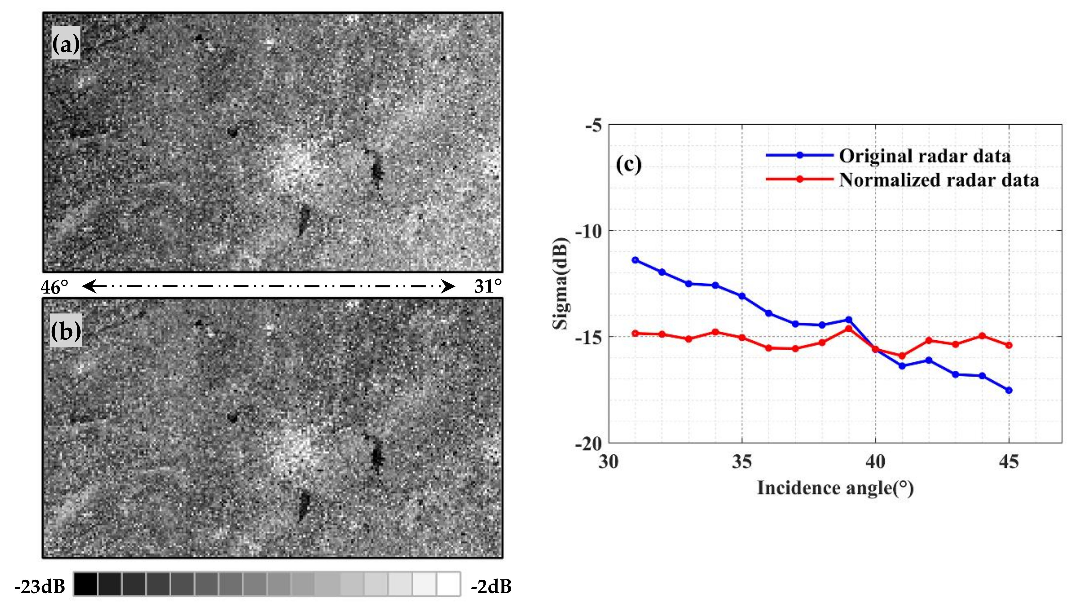
3.2. The Comparison of Sentinel-1 Images before and after Normalization

According to the results of Section 3.1, the dynamic cosine method based on NDVI was established. The image of April 19th (DOY = 109) was selected for the bare soil period. The image of August 17th (DOY = 229) was selected during the tassel to silking period. The images from two periods were normalized to 40° and the effects before and after normalization using the dynamic cosine method were compared (Figure 7 and Figure 8). In the bare soil period, the normalized image (Figure 7b) has good stability and does not change with θ. The raw radar image (Figure 7a) has a significant difference in the radar intensity at close (low incident angle) and long range (high incident angle). The radar echo is strong at close range, and will gradually weaken as it moves to long range. In addition, the radar data before and after normalization were selected to study the changes in σ0 with θ. The average value of σ0 is calculated for the study area at intervals of 1°. In Figure 7, the angle dependence of the normalized radar data is significantly reduced. At low θ, σ0 decreases after normalization and this trend is opposite at high θ. In Figure 8, ∆σ0 is small during the tassel to silking period. σ o b s 0 and σ n o r m 0 have little difference. However, the accuracy of σ n o r m 0 has improved, comparing with σ o b s 0 . The newly proposed method can effectively improve the incidence angle effect of σ o b s 0 .

3.3. Performance Comparison of Three Normalization Methods

To compare the performance for first-order cosine method, cosine square law method and dynamic cosine method, three normalized reference angles (34°, 40°, and 44°) were selected. The results under different polarization and reference angles were analyzed.
The results of dynamic cosine method are in good agreement with σ o b s 0 (Figure 9). Regardless of the two polarizations or the three angles, the performance of dynamic cosine method is better than the other two methods. The results normalized to 34° and 44° are in the appendix (Figure A1). For the performance of the full growth stage of maize, the first-order cosine method and cosine square law normalization method performed well during the tassel to silking period (DOY:193–265). The normalization result at this stage is similar to the dynamic cosine method. During the bare soil period, the seedling emergence to tassel period and the maturity period (April, May, June, and October), σ n o r m 0 based on first-order cosine method and cosine square law method are quite different from σ o b s 0 , and σ n o r m 0 has a relatively large ∆σ0. The dynamic cosine method reduces ∆σ0 to a large extent and shows a good normalization effect.
The overall RMSE and bias normalized to 34°, 40°, and 44° for VV and VH polarization were calculated (Figure 10 and Figure 11). This shows that the overall normalization ability of the dynamic cosine method based on NDVI is significantly better than the above two traditional methods. The overall RMSE and bias of the dynamic cosine method at VV polarization are 0.51 dB and 0.01 dB, respectively, which are 0.50 dB and −0.1 dB at VH polarization.
The overall RMSE of first-order cosine method is 1.51 dB at VV polarization, and bias is −0.17 dB. The overall RMSE and bias of this method at VH polarization are 1.22 dB and −0.24 dB. The overall RMSE and bias of cosine square law method at VV polarization are 1.21 dB and −0.12 dB, respectively, which are 0.94 dB and −0.19 dB at VH polarization. In general, the overall performance of first-order cosine method does not perform well. When σ v v 0 is normalized to 44°, the RMSE reaches the maximum value (4.01 dB) and the bias is −3.23 dB (Figure 10e,f). There is a significant negative deviation between σ n o r m 0 and σ o b s 0 (Figure 12). Cosine square law method is slightly better than that of the first-order cosine method. When σ v v 0 is normalized to 44°, the maximum RMSE is 3.56 dB, and the bias is −2.86 dB (Figure 10e,f). In addition, the maximum RMSE (1.43 dB) of the dynamic cosine method appears when σ v h 0 is normalized to 44° (DOY = 133), and the bias is −1.11 dB. In different polarizations, maize growth stages and θnorm combinations, comparing the overall and maximum RMSE of the three methods, can illustrate the advantages and disadvantages of the normalization method.
Based on the above analysis, the dynamic cosine method meets the normalization requirements of the incident angle better at different maize growth stages. Therefore, this new method tends to perform better than the other two methods.

4. Discussion

4.1. Dynamic Cosine Method Evaluation Within Different Crop Growth Periods and Radar Incidence Angles

A dynamic cosine method based on NDVI has been proposed, which is suitable for different growth stages of maize and the bare soil period (Figure 10 and Figure 11). It expands the applicability of the cosine method. NDVI is used as a factor to characterize the growth stage of maize, and accurate angle normalization is achieved according to it. The results show that the applicability of the dynamic cosine method is different in the bare soil period and the non-bare soil period (Figure 10 and Figure 11). In the bare soil period, the RMSE and bias of dynamic cosine method are larger than those in the non-bare soil period because NDVI is less sensitive to the bare soil period compared with the vegetation period. In addition, spring farming causes farmland blocks to be abnormally broken, and the roughness changes greatly in a short period of time. This is also an important factor affecting the performance of the dynamic cosine method in the bare soil period. The effect of roughness will be described in detail in Section 4.2.
The performance of the dynamic cosine method was evaluated by normalizing the time series SAR images to three representative θnorm. The RMSE of σ v v 0 normalized to 34°, 40°, and 44° is 0.51, 0.47, 0.55 dB, and bias is 0.12, −0.17, and 0.08 dB, respectively. The RMSE of σ v h 0 normalized to 34°, 40°, and 44° is 0.46, 0.48, and 0.58 dB, and bias is 0.08, −0.13, and −0.26 dB. The RMSE of σ v v 0 normalized to 40° is better than that of the other two angles. The RMSE of σ v h 0 normalized to 40° is slightly lower than the value of 34°, which is also an acceptable range. It is worth mentioning that the RMSE of σ v v 0 and σ v h 0 normalized to 44° both showed poor performance. However, with 40° as the normalized reference angle, the results of VV and VH polarization both performed better. Topouzelis et al. (2016) believed that the normalized method based on the cosine law usually works relatively well in the middle of the image, but does not perform correctly at the edges of the range direction [38]. This conclusion is applicable when θnorm is the central θ of an image. The research results found that when θnorm is determined, as the angle difference between θ and θnorm increases the error of σ n o r m 0 also increases. Therefore, the smaller the angle difference from θnorm, the higher the accuracy of σ n o r m 0 . Hence, when normalizing θ of an image, in order to balance the accuracy of σ n o r m 0 for the entire image, the central θ is still the best choice for θnorm. Generally speaking, the dynamic cosine method has greatly reduced this marginal error compared with the two traditional cosine normalization methods. It makes the RMSE of normalized result at the range edge (referring to a larger angle difference from θnorm) within an acceptable range.

4.2. The Influence of Soil Surface Roughness and Soil Moisture on Radar Incidence Angle Effect

Roughness (root mean square height, RMSH) and soil moisture (SM) will affect the dependence of σ0 and θ [15,39]. In the bare soil stage, to analyze the influence of RMSH and SM on our study, the IEM model was used to simulate σ0 (VV and HV polarization) under different incident angles, different RMSH, and different SM. θ is set to 20°–50°, and the interval is 10°; the SM is set to 0.05–0.25 cm3/cm3, and the interval is 0.1 cm3/cm3; and the RMSH is set to 0.25–1.5 cm, and the interval is 0.25 cm. The correlation length is set to 10 cm. For the same SM and RMSH, σ0 at different θ are fitted to obtain N (the method is the same as in Section 2.2.2) and the results of N are shown in Figure 12.
When analyzing the influence of the SM on N in the bare soil stage, the RMSH is fixed. For VV polarization, when the RMSH is less than or equal to 0.75 cm, N decreases with the increase in SM; when the RMSH is greater than 0.75 cm, the trend is the opposite. For HV polarization, N decreases with increasing SM, although this trend is weak. When the RMSH is fixed, the change of N caused by SM is 0.48 and 0.09 for VV and HV polarization, respectively. Therefore, it can be considered that the influence of SM on N is weak. When analyzing the influence of RMSH on N, the SM is fixed. For VV and HV polarization, N decreases as the RMSH increases. Under VV polarization, RMSH has a greater influence on N. When SM is 0.05 cm3/cm3, N corresponding to RMSH (0.25–1.5 cm) is 5.72–1.38, and the change range of N is 4.34. Under HV polarization, N is slightly affected by RMSH. When SM is 0.05 cm3/cm3, N corresponding to RMSH (0.25–1.5 cm) is 2.65–2.16, and the variation range of N is 0.49. This is quite different from the results obtained from satellite data ( σ v h 0 ). However, numerous studies have observed varying degrees of discretions between IEM simulations and SAR data in cross polarization. This discrepancy was related to the model itself [40,41,42].
The simulation experiment based on IEM proves that RMSH has an influence on N, and the influence of SM on N is negligible in the bare soil stage. In the sparse vegetation stage, the influence of vegetation is small, and the characteristics of the bare soil stage are assumed to be applicable in the sparse vegetation stage. N (Section 2.2.2) is obtained by empirical fitting based on the actual radar data in the study area. N mainly includes the influence of vegetation growth stage and part of the influence of RMSH in the bare soil stage. Most of the predecessors regard the RMSH as the focus on the radar incidence angle effect. However, the vegetation growth stage is an important factor affecting radar incidence angle effect, and it is also the focus of this research. The common mechanism of vegetation growth stage and RMSH on N and their specific contributions need to be further studied.

4.3. The Prospects of Dynamic Cosine Methods

The empirical relationship of the dynamic cosine method with the sentinel-1 C-band for maize, and other crops (such as wheat and soybeans) have similar relationships. The new method can even be used in other bands (L-band, X-band). The growth stages of maize can be well characterized by NDVI, which enables the dynamic cosine method based on NDVI to normalize the incidence angle effect at different maize growth stages. However, NDVI is obtained from optical images, which has the inherent defect of optical remote sensing. The effective acquisition of NDVI is limited to almost cloudless conditions, which limits its application in some cases. At present, the radar vegetation index shows great potential in capturing the crop phenological stages [43,44]. For example, the DpRVI (dual-pol radar vegetation index) proposed by Mandal based on Sentinel-1 SAR data can better characterize the growth status of soybeans, wheat, and other crops throughout the crop growth cycle [35]. The acquisition of DpRVI is not restricted by weather conditions (such as clouds and rain), and has great potential. Nevertheless, the applicability of DpRVI in maize needs to be further verified.

5. Conclusions

The normalization accuracy of first-order cosine method and cosine square law method cannot meet the requirements for normalization of the radar incident angle at different growth stages of maize. In order to solve this problem, a dynamic cosine method based on NDVI is proposed with the C-band SAR data (VV and VH polarization), and the accuracy of this method is compared with the traditional cosine method. The conclusion is as follows:
(1) Incidence angle effect (∆σ0) is affected by maize seasonality. During the whole growth stage of maize, the power exponent N in the cosine method dynamically changes in time series SAR images. In the bare soil period (DOY: 109–181, 277–289), the range of N under VV polarization is 4.22–9.35, and under VH polarization is 3.68–6.26. In the vegetation period (DOY: 193–265), the range of N under VV polarization is 0.66–3.35, and under VH polarization is 0.99–3.32.
(2) There is a good correlation between N of dynamic cosine method and NDVI in the maize farmland area of Northeast China. NDVI can be used to parameterize changes in N. The three fitting results have good correlation, and NDVI can realize the dynamic normalization of the incident angle well.
(3) The dynamic cosine method based on NDVI greatly reduces the angular dependence, and has strong robustness in the entire growth stage of maize and different θnorm. For VV polarization, the accuracy of the dynamic cosine method is 66% and 58% higher than that of the first-order cosine method and the cosine square law method, respectively. For VH polarization, the accuracy is improved by 59% and 47%.
At present, the dynamic cosine method based on NDVI performs well in verifying maize crops under C-band SAR data. The concept of dynamic cosine method is also applicable to other wavebands and ground object types. The detailed mechanism of action requires further study.

Author Contributions

Conceptualization, X.Z. and Z.F.; methodology, X.Z. and Z.F.; validation, Z.F; formal analysis, L.L.; resources, B.L.; data curation, S.C.; writing—original draft preparation, Z.F.; writing—review and editing, X.Z. and Z.F.; supervision, T.G.; supervision, X.W.; supervision, T.J.; supervision, X.L. (Xiaofeng Li); and visualization, X.L. (Xiaojie Li). All authors have read and agreed to the published version of the manuscript.

Funding

This research was funded by the National Natural Science Foundation of China, grant number 41971323 and 41771400.

Institutional Review Board Statement

Not applicable.

Informed Consent Statement

Not applicable.

Data Availability Statement

Publicly available datasets were analyzed in this study. This data can be found here: [https://scihub.copernicus.eu/dhus/#/home (accessed on 01 June 2021)].

Conflicts of Interest

The authors declare no conflict of interest.

Appendix A

Figure A1. Comparison of three normalization algorithms from April to October. (a) is the normalization of VV polarization to 34°; (b) is the normalization of VH polarization to 34°; (c) is the normalization of VV polarization to 44°; (d) is the normalization of VH polarization to 44°.
Remotesensing 13 02856 g0a1aRemotesensing 13 02856 g0a1bRemotesensing 13 02856 g0a1c

References

  1. Vreugdenhil, M.; Wagner, W.; Bauer-Marschallinger, B.; Pfeil, I.; Teubner, I.; Rüdiger, C.; Strauss, P. Sensitivity of Sentinel-1 backscatter to vegetation dynamics: An Austrian case study. Remote Sens. 2018, 10, 1396. [Google Scholar] [CrossRef] [Green Version]
  2. Zhou, C.; Zheng, L. Mapping radar glacier zones and dry snow line in the Antarctic Peninsula using Sentinel-1 images. Remote Sens. 2017, 9, 1171. [Google Scholar] [CrossRef] [Green Version]
  3. Zheng, X.; Feng, Z.; Xu, H.; Sun, Y.; Li, L.; Li, B.; Jiang, T.; Li, X.; Li, X. A New Soil Moisture Retrieval Algorithm from the L-Band Passive Microwave Brightness Temperature Based on the Change Detection Principle. Remote Sens. 2020, 12, 1303. [Google Scholar] [CrossRef] [Green Version]
  4. Wang, Y.; Day, J.L.; Davis, F.W.; Melack, J.M. Modeling L-band radar backscatter of Alaskan boreal forest. IEEE Trans. Geosci. Remote Sens. 1993, 31, 1146–1154. [Google Scholar] [CrossRef] [Green Version]
  5. Aldenhoff, W.; Eriksson, L.E.; Ye, Y.; Heuzé, C. First-Year and Multiyear Sea Ice Incidence Angle Normalization of Dual-Polarized Sentinel-1 SAR Images in the Beaufort Sea. IEEE JSTARS 2020, 13, 1540–1550. [Google Scholar] [CrossRef]
  6. Hallikainen, M.; Toikka, M. Classification of sea ice types with radar. In Proceedings of the 1992 22nd European Microwave Conference, Helsinki, Finland, 5–9 September 1992; Volume 2, pp. 957–962. [Google Scholar]
  7. Makynen, M.P.; Manninen, A.T.; Simila, M.H.; Karvonen, J.A.; Hallikainen, M.T. Incidence angle dependence of the statistical properties of C-band HH-polarization backscattering signatures of the Baltic Sea ice. IEEE Trans. Geosci. Remote Sens. 2002, 40, 2593–2605. [Google Scholar] [CrossRef]
  8. Xu, S.; Qi, Z.; Li, X.; Yeh, A.G.O. Investigation of the effect of the incidence angle on land cover classification using fully polarimetric SAR images. Int. J. Remote Sens. 2019, 40, 1576–1593. [Google Scholar] [CrossRef]
  9. Zheng, X.; Feng, Z.; Xu, H.; Sun, Y.; Bai, Y.; Li, B.; Li, L.; Zhao, X.; Zhang, R.; Jiang, T.; et al. Performance of four passive microwave soil moisture products in maize cultivation areas of Northeast China. IEEE JSTARS 2020, 13, 2451–2460. [Google Scholar]
  10. Mladenova, I.E.; Jackson, T.J.; Bindlish, R.; Hensley, S. Incidence angle normalization of radar backscatter data. IEEE Trans. Geosci. Remote Sens. 2012, 51, 1791–1804. [Google Scholar] [CrossRef]
  11. Lang, W.; Zhang, P.; Wu, J.; Shen, Y.; Yang, X. Incidence angle correction of SAR sea ice data based on locally linear mapping. IEEE Trans. Geosci. Remote Sens. 2016, 54, 3188–3199. [Google Scholar] [CrossRef]
  12. Fore, A.G.; Chapman, B.D.; Hawkins, B.P.; Hensley, S.; Jones, C.E.; Michel, T.R.; Muellerschoen, R.J. UAVSAR polarimetric calibration. IEEE Trans. Geosci. Remote Sens. 2015, 53, 3481–3491. [Google Scholar] [CrossRef]
  13. Ye, N.; Walker, J.P.; Rüdiger, C. A cumulative distribution function method for normalizing variable-angle microwave observations. IEEE Trans. Geosci. Remote Sens. 2015, 53, 3906–3916. [Google Scholar] [CrossRef]
  14. Wu, X.; Walker, J.P.; Das, N.N.; Panciera, R.; Rüdiger, C. Evaluation of the SMAP brightness temperature downscaling algorithm using active–passive microwave observations. Remote Sens. Environ. 2014, 155, 210–221. [Google Scholar] [CrossRef]
  15. Ulaby, F.T.; Moore, R.K.; Fung, A.K. Radar remote sensing and surface scattering and emission theory. In Microwave Remote Sensing: Active and Passive; Addison-Wesley: Boston, MA, USA, 1982; Volume 2, pp. 194–246. [Google Scholar]
  16. Widhalm, B.; Bartsch, A.; Goler, R. Simplified normalization of C-band synthetic aperture radar data for terrestrial applications in high latitude environments. Remote Sens. 2018, 10, 551. [Google Scholar] [CrossRef] [Green Version]
  17. Clapp, R.E. A Theoretical and Experimental Study of Radar Ground Return; Radiation Laboratory, Massachusetts Institute of Technology: Cambridge, MA, USA, 1946. [Google Scholar]
  18. Ardila, J.P.; Tolpekin, V.; Bijker, W. Angular backscatter variation in L-band ALOS ScanSAR images of tropical forest areas. IEEE Geosci. Remote Sens. Lett. 2010, 7, 821–825. [Google Scholar] [CrossRef] [Green Version]
  19. Quiñones, M.J.; Hoekman, D.H. Exploration of factors limiting biomass estimation by polarimetric radar in tropical forests. IEEE Trans. Geosci. Remote Sens. 2004, 42, 86–104. [Google Scholar] [CrossRef]
  20. Guo, P.; Zhao, T.; Shi, J.; Xu, H.; Li, X.; Niu, S. Assessing the active-passive approach at variant incidence angles for microwave brightness temperature downscaling. Int. J. Digit. Earth 2021, 7, 1–21. [Google Scholar] [CrossRef]
  21. Zribi, M.; Chahbi, A.; Shabou, M.; Lili-Chabaane, Z.; Duchemin, B.; Baghdadi, N.; Amri, R.; Chehbouni, A. Soil surface moisture estimation over a semi-arid region using ENVISAT ASAR radar data for soil evaporation evaluation. Hydrol. Earth Syst. Sci. 2011, 15, 345–358. [Google Scholar] [CrossRef] [Green Version]
  22. Baghdadi, N.; Bernier, M.; Gauthier, R.; Neeson, I. Evaluation of C-band SAR data for wetlands mapping. Int. J. Remote Sens. 2001, 22, 71–88. [Google Scholar] [CrossRef]
  23. Huang, W.; Sun, G.; Ni, W.; Zhang, Z.; Dubayah, R. Sensitivity of multi-source SAR backscatter to changes in forest aboveground biomass. Remote Sens. 2015, 7, 9587–9609. [Google Scholar] [CrossRef] [Green Version]
  24. Menges, C.H.; Van Zyl, J.J.; Hill, G.J.; Ahmad, W. A procedure for the correction of the effect of variation in incidence angle on AIRSAR data. Int. J. Remote Sens. 2001, 22, 829–841. [Google Scholar] [CrossRef]
  25. Doninck, J.V.; Wagner, W.; Melzer, T.; De Baets, B.; Verhoest, N.E. Seasonality in the Angular Dependence of ASAR Wide Swath Backscatter. IEEE Geosci. Remote Sens. Lett. 2014, 11, 1423–1427. [Google Scholar] [CrossRef]
  26. Cristea, A.; van Houtte, J.; Doulgeris, A.P. Integrating incidence angle dependencies into the clustering-based segmentation of SAR images. IEEE JSTARS 2020, 13, 2925–2939. [Google Scholar]
  27. Fieuzal, R.; Baup, F.; Marais-Sicre, C. Monitoring wheat and rapeseed by using synchronous optical and radar satellite data—From temporal signatures to crop parameters estimation. Adv. Remote Sens. 2013, 2, 162–180. [Google Scholar] [CrossRef] [Green Version]
  28. Li, X.; Li, H.; Yang, L.; Ren, Y. Assessment of soil quality of croplands in the Corn Belt of Northeast China. Sustainability 2018, 10, 248. [Google Scholar] [CrossRef] [Green Version]
  29. Gong, Z.J.; Liu, L.M.; Chen, J. Phenophase extraction of spring maize in Liaoning province based on MODIS NDVI data. J. Shenyang Agric. Univ. 2018, 49, 257–265. [Google Scholar]
  30. Li, Y.; Zhang, C.C.; Luo, W.R.; Gao, W.J. Summer maize phenology monitoring based on normalized difference vegetation index reconstructed with improved maximum value composite. Transact. CSAE 2019, 35, 159–165. [Google Scholar]
  31. Chen, J.; Jönsson, P.; Tamura, M.; Gu, Z.; Matsushita, B.; Eklundh, L. A simple method for reconstructing a high-quality NDVI time-series data set based on the Savitzky–Golay filter. Remote Sens. Environ. 2004, 91, 332–344. [Google Scholar] [CrossRef]
  32. Zhao, X.W. Soil Moisture Retrieval Using SAR Data in Agricultural Areas based on Change Detection Approach. Master’s Thesis, Jilin University, Jilin, China, 2019. [Google Scholar]
  33. O’Grady, D.; Leblanc, M.; Gillieson, D. Relationship of local incidence angle with satellite radar backscatter for different surface conditions. Int. J. Appl. Earth Obs. Geoinf. 2013, 24, 42–53. [Google Scholar] [CrossRef]
  34. Mo, L. Quantitative Research and Correction of Incident Angle Effect for Wide Swath SAR Image. Master’s Thesis, Hefei University of Technology, Anhui, China, 2013. [Google Scholar]
  35. Mandal, D.; Kumar, V.; Ratha, D.; Dey, S.; Bhattacharya, A.; Lopez-Sanchez, J.M.; McNairn, H.; Rao, Y.S. Dual polarimetric radar vegetation index for crop growth monitoring using sentinel-1 SAR data. Remote Sens. Environ. 2020, 247, 111954. [Google Scholar] [CrossRef]
  36. Wagner, W.; Noll, J.; Borgeaud, M.; Rott, H. Monitoring soil moisture over the Canadian Prairies with the ERS scatterometer. IEEE Trans. Geosci. Remote Sens. 1999, 37, 206–216. [Google Scholar] [CrossRef]
  37. Pittman, K.; Hansen, M.C.; Becker-Reshef, I.; Potapov, P.V.; Justice, C.O. Estimating global cropland extent with multi-year MODIS data. Remote Sens. 2010, 2, 1844–1863. [Google Scholar] [CrossRef] [Green Version]
  38. Topouzelis, K.; Singha, S.; Kitsiou, D. Incidence angle normalization of Wide Swath SAR data for oceanographic applications. Open Geosci. 2016, 8, 450–464. [Google Scholar] [CrossRef] [Green Version]
  39. Zheng, X.; Feng, Z.; Li, L.; Li, B.; Jiang, T.; Li, X.; Li, X.; Chen, S. Simultaneously estimating surface soil moisture and roughness of bare soils by combining optical and radar data. Int. J. Appl. Earth Obs. Geoinf. 2021, 100, 102345. [Google Scholar] [CrossRef]
  40. Baghdadi, N.; Zribi, M. Evaluation of radar backscatter models IEM, OH and Dubois using experimental observations. Int. J. Remote Sens. 2006, 27, 3831–3852. [Google Scholar] [CrossRef]
  41. Baghdadi, N.; Holah, N.; Zribi, M. Calibration of the integral equation model for SAR data in C-band and HH and VV polarizations. Int. J. Remote Sens. 2006, 27, 805–816. [Google Scholar] [CrossRef]
  42. Baghdadi, N.; Abou Chaaya, J.; Zribi, M. Semiempirical calibration of the integral equation model for SAR data in C-band and cross polarization using radar images and field measurements. IEEE Geosci. Remote Sens. Lett. 2010, 8, 14–18. [Google Scholar] [CrossRef] [Green Version]
  43. Veloso, A.; Mermoz, S.; Bouvet, A.; Le Toan, T.; Planells, M.; Dejoux, J.F.; Ceschia, E. Understanding the temporal behavior of crops using Sentinel-1 and Sentinel-2-like data for agricultural applications. Remote Sens. Environ. 2017, 199, 415–426. [Google Scholar] [CrossRef]
  44. Khabbazan, S.; Vermunt, P.; Steele-Dunne, S.; Ratering Arntz, L.; Marinetti, C.; van der Valk, D.; Iannini, L.; Molijn, R.; Westerdijk, K.; van der Sande, C. Crop monitoring using Sentinel-1 data: A case study from The Netherlands. Remote Sens. 2019, 11, 1887. [Google Scholar] [CrossRef] [Green Version]
Figure 1. Location of the study area. (a) The red box represents the scope of the study area, which is located in the farmland area in the middle of Jilin Province; (b) the digital elevation map of the study area; and (c) the land cover classification from GlobeLand30 (http://www.globallandcover.com (accessed on 01 June 2021)).
Remotesensing 13 02856 g001
Figure 2. The multi-temporal Sentinel-1 VV polarization backscattering coefficient after being pre-processed in the study area. The incidence angle of each image is 31–46° from right to left.
Remotesensing 13 02856 g002
Figure 3. The statistical relationship between radar backscattering coefficient (σ0) and the incident angle from April to October. (a) VV polarization; (b) VH polarization.
Remotesensing 13 02856 g003
Figure 4. The combination of normalized angle for least squares fitting.
Remotesensing 13 02856 g004
Figure 5. Time series relationship between Nvv, Nvh, and NDVI. Nvv (Nvh) represents the N value under VV (VH) polarization.
Remotesensing 13 02856 g005
Figure 6. Regression relationship between N and NDVI for VV and VH polarization. (a) and (d): linear; (b) and (e): logarithmic; and (c) and (f): exponential.
Remotesensing 13 02856 g006
Figure 7. Comparison of VV polarizations for C bands showing the raw (a) and normalized (b) radar data (19th April, DOY = 109). (c) represents the radar data before and after normalization in the study area.
Remotesensing 13 02856 g007
Figure 8. Comparison of VV polarizations for C bands showing the raw (a) and normalized (b) radar data (17th August, DOY = 229). (c) represents the radar data before and after normalization in the study area.
Remotesensing 13 02856 g008
Figure 9. The comparison of σ o b s 0 and σ n o r m 0 normalized to 40° by first-order cosine normalization, cosine square law normalization, and dynamic cosine method from April to October. (a) VV polarization; (b) VH polarization.
Remotesensing 13 02856 g009aRemotesensing 13 02856 g009b
Figure 10. The RMSE and bias of first-order cosine method, cosine square law method, and dynamic cosine method (VV polarization). (a), (c), and (e) represent the RMSE for 34°, 40°, and 44°, respectively; (b), (d), and (f) respectively represent the deviation bias for 34°, 40°, and 44°.
Remotesensing 13 02856 g010
Figure 11. The same as Figure 10 but for VH polarization.
Remotesensing 13 02856 g011
Figure 12. The influence of soil moisture and soil surface roughness parameter (root mean square height, RMSH) on N. (a) VV polarization; (b) HV polarization.
Remotesensing 13 02856 g012
Table 1. The difference of backscattering coefficients (∆σ0) corresponding to incident angles of 31° and 46° in the time series Sentinel-1 C-band radar data.
Sentinel-1 Acquisition DateDOY σ v v 0 (31°) σ v v 0 (46°) σ v v 0 σ v h 0 (31°) σ v h 0 (46°) σ v h 0
2019-04-19109−11.06−17.116.05−20.22−22.902.68
2019-05-13133−9.23−17.027.79−18.47−22.834.35
2019-06-06157−9.12−15.296.17−18.49−21.493.00
2019-06-18169−9.44−13.263.82−17.56−20.583.02
2019-06-30181−7.04−10.443.41−13.91−17.213.30
2019-07-12193−7.97−10.282.31−14.22−16.932.71
2019-07-24205−7.95−9.901.95−14.07−15.731.66
2019-08-17229−8.04−9.291.25−14.10−15.050.94
2019-09-10253−8.09−11.163.07−15.06−16.951.90
2019-09-22265−8.42−11.593.17−15.16−17.752.59
2019-10-04277−9.02−12.993.97−15.52−19.654.13
2019-10-16289−9.92−14.955.03−18.07−21.533.46
Note: The unit of backscattering coefficients is dB.
Table 2. The fitted accuracy (R2 and RMSE) and N value for σ v v 0 and σ v h 0 during DOY of 109–289, and the corresponding NDVI value was computed from Sentinel-2 reflectance.
VVVH
DataDOYNR2RMSENR2RMSENDVI
2019-04-191097.020.950.1914.690.690.3270.15
2019-05-131339.350.910.4176.260.720.4410.17
2019-06-061577.470.890.3194.820.740.2960.23
2019-06-181694.220.900.1423.680.960.0740.27
2019-06-301814.300.940.1084.060.970.0680.48
2019-07-121932.900.980.0423.320.970.0540.71
2019-07-242051.830.880.0661.610.960.0310.75
2019-08-172290.660.240.1100.990.810.0460.83
2019-09-102533.060.960.0642.100.890.0720.78
2019-09-222653.350.990.0353.090.990.0370.59
2019-10-042774.630.980.0704.830.980.0640.40
2019-10-162895.850.970.1224.610.910.1510.28
Publisher’s Note: MDPI stays neutral with regard to jurisdictional claims in published maps and institutional affiliations.

