The Analysis of Fractional-Order Kersten–Krasil Shchik Coupled KdV System, via a New Integral Transform

Abstract

In this article, we use the homotopy perturbation transform method to find the fractional Kersten–Krasil’shchik coupled Korteweg–de Vries (KdV) non-linear system. This coupled non-linear system is typically used to describe electric circuits, traffic flow, shallow water waves, elastic media, electrodynamics, etc. The homotopy perturbation method is modified with the help of the $\rho$-Laplace transformation to investigate the solution of the given examples to show the accuracy of the current technique. The solution of the given technique and the actual results are shown and analyzed with figures.

1. Introduction

Fractional calculus has a long history that began at the end of the 17 century and continued until the 20th century. Many scientists and mathematicians have spent the last few decades researching numerical and analytic results to nonlinear fractional partial differential equations in engineering and science. Due to their use in many implementations, such as viscoelasticity, fluid mechanic, physics, biology, dynamic schemes of control theories, electric networks, optics, chemical physics, and signal processing, fractional differential equations have gained special attention. Many books contain various definitions and basic concepts of fractional calculus [1,2,3,4].

A differential equation symmetry is a transformation that makes the differential equation invariant. The existence of such symmetries may aid in the solution of the differential equation. A scheme of differential equations line symmetry is a continous symmetry of a scheme of differential equations. Solving a linked set of ordinary differential equations can reveal symmetries. It is sometimes easier to solve these equations than it is to solve the original differential equations. The symmetry structure of the system consists of integer partial differential equations and fractional-order partial differential equations with the fractional Caputo derivative.

Using the symmetry construction, we consider two particular cases: pure fractional-order partial differential equations, whose symmetry condition is divided into two parts of integer-order and fractional, and the linear scheme of fractional partial differential equations, which acknowledges an infinite dimensional insignificant generator continuously. Second, we built a theoretical structure of potential symmetry and constructed three potential schemes to analyze potential symmetries of time-fractional partial differential equations with a divergence form using the composition rule of fractional derivatives. Still, when dealing with linear equations, it is impossible to find their exact results.

Therefore, many approximate and numerical methods have been introduced for the results of fractional-order linear and non-linear differential equations, such as variation iteration technique [5,6], Adomian’s decomposition technique [7], homotopy analysis technique [8], homotopy perturbation technique [9], differential transform technique [10], homotopy asymptotic technique [11], and Galerkin technique [12].

The fractional coupled Kersten–Krasil’shchik Korteweg–de Vries (KdV) nonlinear scheme and homogeneous two component fractional coupled third-order KdV schemes are significant fractional-order nonlinear systems for identifying wave behavior elaborating numerous nonlinear phenomena in physics. The fractional-order coupled system is widely used to investigate complex behavior containing multi-components, such as atoms, ions, and free electrons. Many scholars have attempted to study this behavior numerically.

Recently, Paul Kersten and Joseph Krasil’shchik analyzed and modified the KdV equation, proposing absolute complexity between coupled KdV nonlinear systems to analyze the behavior of nonlinear systems. Numerous variations of this Kersten–Krasil’shchik coupled KdV-mKdV nonlinear system have been introduced by many researchers [13,14,15,16]. Many researchers applied different analytical and numerical methods to investigate KdV equations, such as the homotopy analysis method [17], expansion method [18], shifted Legendre polynomials [19], and natural decomposition method [20].

The homotopy perturbation method (HPM) was first proposed by He [21]. For solving differential and integral equations, linear and nonlinear has been the subject abstract and applied analysis of extensive analytical and numerical studies [21]. The HPM is efficient and effective and eliminates an unconditioned matrix, complicated integrals, and infinite series. This method does not need a specific parameter of the model. The $\rho$-Laplace transformation is a modified transformation of the Laplace transform.

It should be remembered that, with the use of $\rho$-Laplace transform, absolute differential equations with variable coefficients cannot be solved by Laplace and Sumudu transforms [22,23]. The homotopy perturbation transformation method (HPTM) combines the $\rho$-Laplace transformation and the homotopy perturbation method. Numerous researchers have utilized HPTM to solve various equations, such as Navier–Stokes problems [24], heat-like problems [25], gas dynamic models [26], and Fisher’s and hyperbolic equation [27].

2. Basic Definitions

In this section, the generalized fractional integral, the generalized fractional derivative, the Mittag–Lefller function, and the $\rho$-Laplace transformation are defined.

Definition 1.

The fractional-order generalized integral ϱ of a continuous function $g:[0,+\infty ]\to R$ is given as [22]

$$\left(I^{\varrho ,\rho }g\right)\left(\chi \right)=\frac{1}{\mathsf{\Gamma }\left(\varrho \right)}{\int }_0^{\chi }{\left(\frac{{\chi }^{\rho }-s^{\rho }}{\rho }\right)}^{\varrho -1}\frac{g\left(s\right)ds}{s^{1-\rho }},$$

the gamma function denote by Γ, $\rho >0$, $\chi >0$ and $0<\varrho <1$.

Definition 2.

The fractional-order generalized derivative of ϱ of a continuous function $g:[0,+\infty ]\to R$ is given as [22]

$$\left(D^{\varrho ,\rho }g\right)\left(\chi \right)=\left(I^{1-\varrho ,\rho }g\right)\left(\chi \right)=\frac{1}{\mathsf{\Gamma }(1-\varrho )}\left(\frac{d}{d\chi }\right){\int }_0^{\chi }{\left(\frac{{\chi }^{\rho }-s^{\rho }}{\rho }\right)}^{-\varrho }\frac{g\left(s\right)ds}{s^{1-\rho }}.$$

where we define the gamma function Γ, $\rho >0$, $\chi >0$ and $0<\varrho <1$.

Definition 3.

The fractional-order Caputo derivative ϱ of a continuous function $g:[0,+\infty ]\to R$ is expressed as [22]

$$\left(D^{\varrho ,\rho }g\right)\left(\chi \right)=\frac{1}{\mathsf{\Gamma }(1-\varrho )}{\int }_0^{\chi }{\left(\frac{{\chi }^{\rho }-s^{\rho }}{\rho }\right)}^{-\varrho }\beta \frac{g\left(s\right)ds}{s^{1-\rho }}.$$

where$\rho >0$, $\chi >0$, $\beta ={\chi }^{1-\rho }\frac{d}{d\chi }$and$0<\varrho <1$.

Definition 4.

The ρ-Laplace transform of a continuous function $g:[0,+\infty ]\to R$ is defined as [22]

$$L_{\rho }\left\{g\left(\chi \right)\right\}={\int }_0^{\infty }{e}^{-s\frac{{\chi }^{\rho }}{\rho }}g\left(\chi \right)\frac{d\chi }{{\chi }^{1-\rho }}.$$

A continuous function g as the fractional-order Caputo generalized rho-Laplace transform derivative is defined by

$$\begin{array}{c}\hfill L_{\rho }\left\{D^{\varrho ,\rho }g\left(\chi \right)\right\}=s^{\varrho }{L}_{\rho }\left\{g\left(\chi \right)\right\}-\sum _{k=0}^{n-1}{s}^{\varrho -k-1}\left(I^{\varrho ,\rho }{\beta }^{n}g\right)\left(0\right).\end{array}$$

3. The General Methodology of HPTM

In this section, the HPTM for the general form of FPDEs

$$\begin{array}{cc}\hfill & D_{\Im }^{\varrho }\phi (\chi ,\Im )+M\phi (\chi ,\Im )+N\phi (\chi ,\Im )=h(\chi ,\Im ),\Im >0,0<\varrho \le 1,\hfill \end{array}$$

(1)

with the initial condition

$$\begin{array}{c}\hfill \phi (\chi ,0)=g\left(\chi \right).\end{array}$$

(2)

where $D_{\Im }^{\varrho }\phi (\chi ,\Im )=\frac{{\partial }^{\varrho }}{\partial {\Im }^{\varrho }}$ is the Caputo fractional derivative of order $\varrho$; M and N, are linear and non-linear functions, respectively; and h is the source operator. Using the $\rho$-Laplace transform of Equation (1),

$$\begin{array}{cc}\hfill & L_{\rho }[D_{\Im }^{\varrho }\phi (\chi ,\Im )+M\phi (\chi ,\Im )+N\phi (\chi ,\Im )]=L_{\rho }\left[h(\chi ,\Im )\right],\Im >0,0<\varrho \le 1,\hfill \\ \hfill & \phi (\chi ,\Im )=\frac{1}{s}g\left(\chi \right)+\frac{1}{s^{\varrho }}{L}_{\rho }\left[h(\chi ,\Im )\right]-\frac{1}{s^{\varrho }}{L}_{\rho }[M\phi (\chi ,\Im )+N\phi (\chi ,\Im )].\hfill \end{array}$$

(3)

Now, by taking inverse $\rho$-Laplace transform, we obtain

$$\phi (\chi ,\Im )={L_{\rho }}^{-1}\left[\frac{1}{s}g\left(\chi \right)+\frac{1}{s^{\varrho }}{L}_{\rho }\left[h(\chi ,\Im )\right]\right]-{L_{\rho }}^{-1}\left[\frac{1}{s^{\varrho }}{L}_{\rho }\{M\phi (\chi ,\Im )+N\phi (\chi ,\Im )\}\right],$$

(4)

where

$$\phi (\chi ,\Im )=g\left(\chi \right)+{L_{\rho }}^{-1}\left[\frac{1}{s^{\varrho }}{L}_{\rho }\left[h(\chi ,\Im )\right]\right]-{L_{\rho }}^{-1}\left[\frac{1}{s^{\varrho }}{L}_{\rho }\{M\phi (\chi ,\Im )+N\phi (\chi ,\Im )\}\right],$$

(5)

Now, the perturbation method parameter p is defined as

$$\phi (\chi ,\Im )=\sum _{𝚥=0}^{\infty }{p}^{𝚥}{\phi }_{𝚥}(\chi ,\Im ),$$

(6)

where the perturbation term $p\in [0,1]$.

The non-linear functions can be defined as

$$N\phi (\chi ,\Im )=\sum _{𝚥=0}^{\infty }{p}^{𝚥}{H}_{𝚥}\left({\phi }_{𝚥}\right),$$

(7)

where $H_m$ are He polynomials of ${\phi }_0,{\phi }_1,{\phi }_2,\cdots ,{\phi }_m,$ and can be determined as

$$H_m({\phi }_0,{\phi }_1,\cdots ,{\phi }_m)=\frac{1}{m!}\frac{{\partial }^m}{\partial p^m}{\left[N\left(\sum _{𝚥=0}^{\infty }{p}^{𝚥}{\phi }_{𝚥}\right)\right]}_{p=0},m=0,1,2\cdots .$$

(8)

putting Equations (7) and (8) in Equation (5), we have

$$\sum _{𝚥=0}^{\infty }{p}^{𝚥}{\phi }_{𝚥}(\chi ,\Im )=g\left(\chi \right)+{L_{\rho }}^{-1}\left[\frac{1}{s^{\varrho }}{L}_{\rho }\left[h(\chi ,\Im )\right]\right]-p\times \left[{L_{\rho }}^{-1}\left\{\frac{1}{s^{\varrho }}{L}_{\rho }\{M\sum _{𝚥=0}^{\infty }{p}^{𝚥}{\phi }_{𝚥}(\chi ,\Im )+\sum _{𝚥=0}^{\infty }{p}^{𝚥}{H}_{𝚥}\left({\phi }_{𝚥}\right)\}\right\}\right].$$

(9)

With both sides comparison coefficient of p, we have

$$\begin{array}{cc}\hfill & p^0:{\phi }_0(\chi ,\Im )=g\left(\chi \right)+{L_{\rho }}^{-1}\left[\frac{1}{s^{\varrho }}{L}_{\rho }\left[h(\chi ,\Im )\right]\right],\hfill \\ \hfill & p^1:{\phi }_1(\chi ,\Im )={L_{\rho }}^{-1}\left[\frac{1}{s^{\varrho }}{L}_{\rho }(M{\phi }_0(\chi ,\Im )+H_0\left(\phi \right))\right],\hfill \end{array}$$

(10)

$$\begin{array}{cc}\hfill & p^2:{\phi }_2(\chi ,\Im )={L_{\rho }}^{-1}\left[\frac{1}{s^{\varrho }}{L}_{\rho }(M{\phi }_1(\chi ,\Im )+H_1\left(\phi \right))\right],\hfill \\ \hfill & ⋮\hfill \\ \hfill & p^{𝚥}:{\phi }_{𝚥}(\chi ,\Im )={L_{\rho }}^{-1}\left[\frac{1}{s^{\varrho }}{L}_{\rho }(M{\phi }_{𝚥-1}(\chi ,\Im )+H_{𝚥-1}\left(\phi \right))\right],𝚥>0,𝚥\in N.\hfill \end{array}$$

(11)

$$\phi (\chi ,\Im )=\underset{M\to \infty }{lim}\sum _{𝚥=1}^M{\phi }_{𝚥}(\chi ,\Im ).$$

(12)

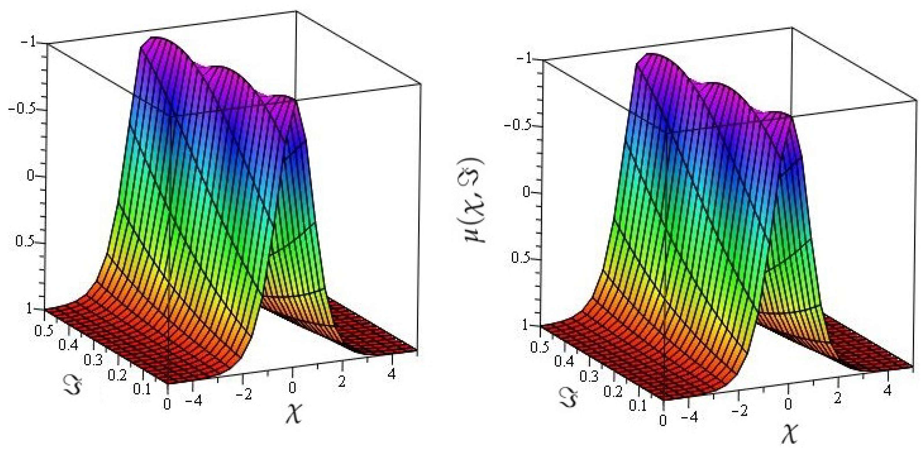
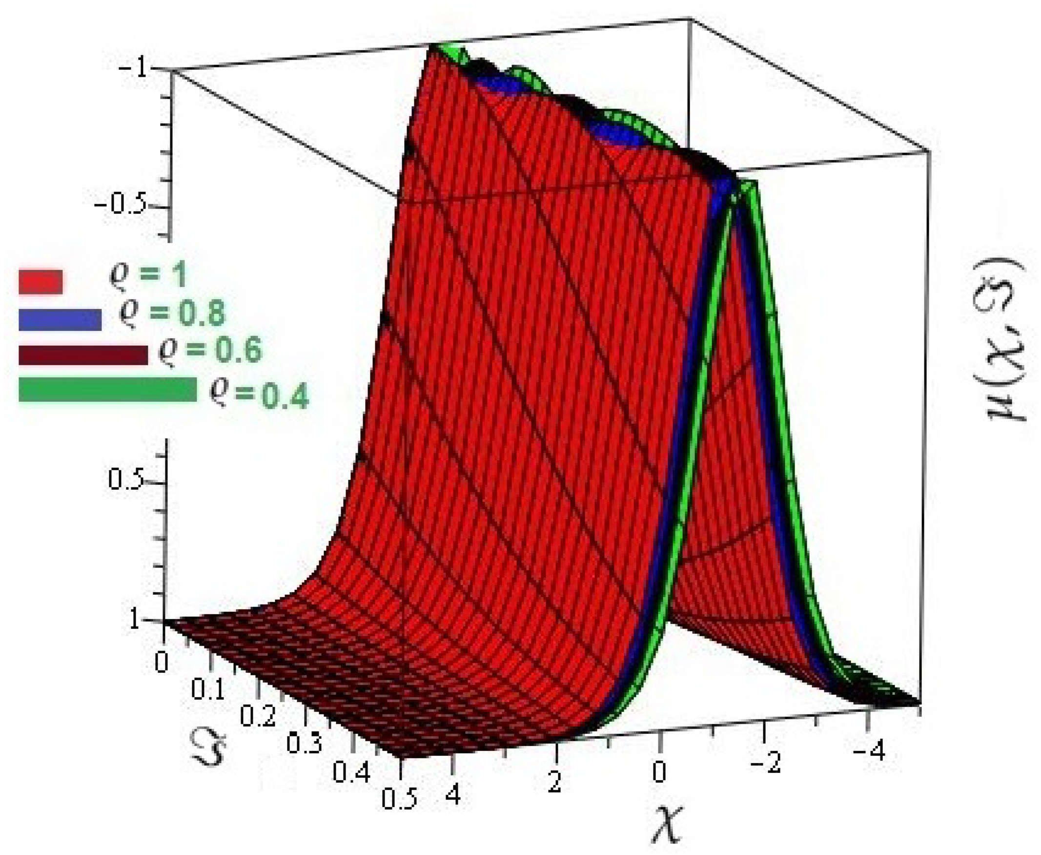
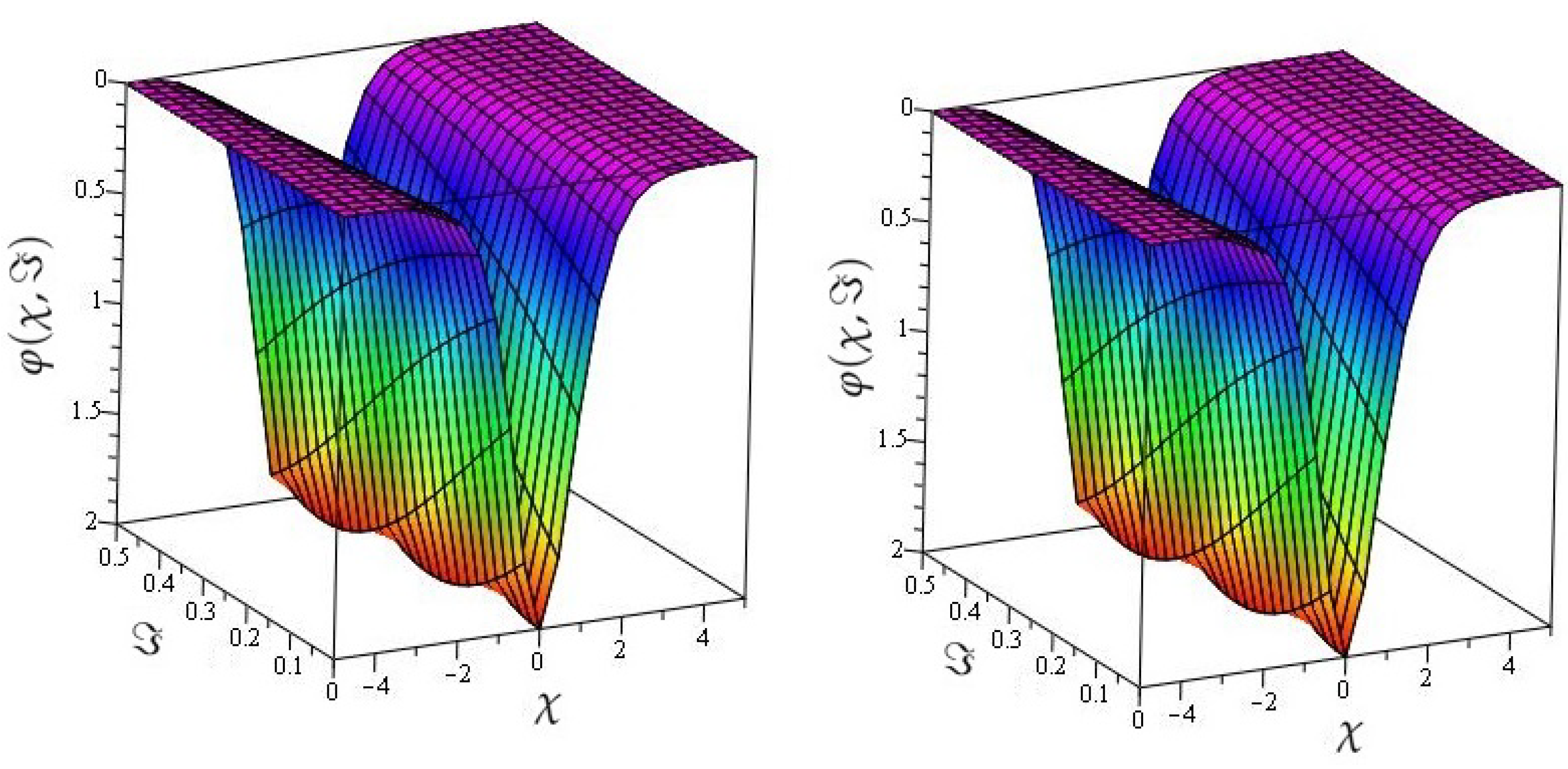
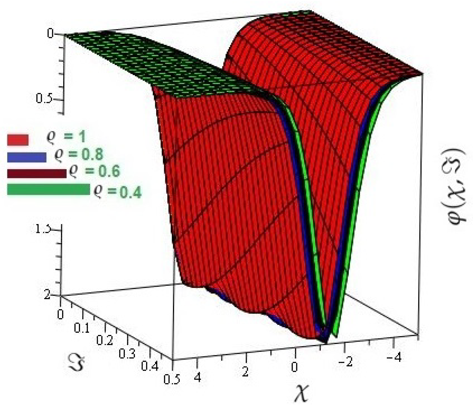
4. Numerical Experiments

Example 1.

Assume time fractional Kersten–Krasil’shchik coupled KdV-mKdV nonlinear system as:

$$\begin{array}{cc}& D_{\Im }^{\varrho }\mu +{\mu }_{3\chi }-6\mu {\mu }_{\chi }+3\phi {\phi }_{3\chi }+3{\phi }_{\chi }{\phi }_{2\chi }-3{\mu }_{\chi }{\phi }^2+6\mu \phi {\phi }_{\chi }=0,\Im >0,\chi \in R,0<\varrho \le 1,\hfill \\ & D_{\Im }^{\varrho }\phi +{\phi }_{3\chi }-3{\phi }^2{\phi }_{\chi }-3\mu {\phi }_{\chi }+3{\mu }_{\chi }\phi =0,\hfill \end{array}$$

(13)

with the initial conditions

$$\begin{array}{cc}\hfill \mu (\chi ,0)=& c-2c{sech}^2\left(\sqrt{c}\chi \right),c>0,\hfill \\ \hfill \phi (\chi ,0)=& 2\sqrt{c}sech\left(\sqrt{c}\chi \right).\hfill \end{array}$$

(14)

Using ρ-Laplace transform on Equation (13) by the application of the initial condition given by Equation (14), we find

$$\begin{array}{cc}\hfill L_{\rho }\left[\mu (\chi ,\Im )\right]& =c-2c{sech}^2\left(\sqrt{c}\chi \right)-\frac{1}{s^{\varrho }}{L}_{\rho }[{\mu }_{3\chi }-6\mu {\mu }_{\chi }+3\phi {\phi }_{3\chi }+3{\phi }_{\chi }{\phi }_{2\chi }-3{\mu }_{\chi }{\phi }^2+6\mu \phi {\phi }_{\chi }],\hfill \\ \hfill L_{\rho }\left[\phi (\chi ,\Im )\right]& =2\sqrt{c}sech\left(\sqrt{c}\chi \right)-\frac{1}{s^{\varrho }}{L}_{\rho }[{\phi }_{3\chi }-3{\phi }^2{\phi }_{\chi }-3\mu {\phi }_{\chi }+3{\mu }_{\chi }\phi ]\hfill \end{array}$$

(15)

Apply the inverse ρ-Laplace transform, and we obtain

$$\begin{array}{cc}\hfill \mu (\chi ,\Im )& =c-2c{sech}^2\left(\sqrt{c}\chi \right)-L_{\rho }^{-1}\left[\frac{1}{s^{\varrho }}{L}_{\rho }[{\mu }_{3\chi }-6\mu {\mu }_{\chi }+3\phi {\phi }_{3\chi }+3{\phi }_{\chi }{\phi }_{2\chi }-3{\mu }_{\chi }{\phi }^2+6\mu \phi {\phi }_{\chi }]\right],\hfill \\ \hfill \phi (\chi ,\Im )& =2\sqrt{c}sech\left(\sqrt{c}\chi \right)-L_{\rho }^{-1}\left[\frac{1}{s^{\varrho }}{L}_{\rho }[{\phi }_{3\chi }-3{\phi }^2{\phi }_{\chi }-3\mu {\phi }_{\chi }+3{\mu }_{\chi }\phi ]\right]\hfill \end{array}$$

(16)

Use HPM on Equation (16), and we obtain

$$\begin{array}{cc}\hfill \sum _{n=0}^{\infty }{p}^n{\mu }_n(\chi ,\Im )& =c-2c{sech}^2\left(\sqrt{c}\chi \right)\hfill \\ \hfill & -p\left(L_{\rho }^{-1}\left[\frac{1}{s^{\varrho }}S\left[{\left(\sum _{n=0}^{\infty }{p}^n{\mu }_n(\chi ,\Im )\right)}_{3\chi }+\left(\sum _{n=0}^{\infty }{p}^n{H}_n\left(\mu \right)\right)\right]\right]\right),\hfill \\ \hfill \sum _{n=0}^{\infty }{p}^n{\phi }_n(\chi ,\Im )& =2\sqrt{c}sech\left(\sqrt{c}\chi \right)\hfill \\ \hfill & -p\left(L_{\rho }^{-1}\left[\frac{1}{s^{\varrho }}S\left[{\left(\sum _{n=0}^{\infty }{p}^n{\phi }_n(\chi ,\Im )\right)}_{3\chi }+\left(\sum _{n=0}^{\infty }{p}^n{H}_n\left(\phi \right)\right)\right]\right]\right)\hfill \end{array}$$

(17)

Nonlinear steps given by He’s polynomials $H_n\left(\mu \right)$ and $H_n\left(\phi \right)$, which are given as

$$\begin{array}{cc}\hfill \sum _{n=0}^{\infty }{p}^n{H}_n\left(\mu \right)& =-6\mu {\mu }_{\chi }+3\phi {\phi }_{3\chi }+3{\phi }_{\chi }{\phi }_{2\chi }-3{\mu }_{\chi }{\phi }^2+6\mu \phi {\phi }_{\chi },\hfill \\ \hfill \sum _{n=0}^{\infty }{p}^n{H}_n\left(\phi \right)& =-3{\phi }^2{\phi }_{\chi }-3\mu {\phi }_{\chi }+3{\mu }_{\chi }\phi .\hfill \end{array}$$

(18)

Values of components of He’s polynomials are given by

$$\begin{array}{cc}\hfill H_0\left(\mu \right)& =-6{\mu }_0{\left({\mu }_0\right)}_{\chi }+3{\phi }_0{\left({\phi }_0\right)}_{3\chi }+3{\left({\phi }_0\right)}_{\chi }{\left({\phi }_0\right)}_{2\chi }-3{\left({\mu }_0\right)}_{\chi }{\left({\phi }_0\right)}^2+6\left({\mu }_0\right){\phi }_0{\left({\phi }_0\right)}_{\chi },\hfill \\ \hfill H_1\left(\mu \right)& =-6{\mu }_1{\left({\mu }_0\right)}_{\chi }-6{\mu }_0{\left({\mu }_1\right)}_{\chi }+3{\phi }_1{\left({\phi }_0\right)}_{3\chi }+3{\phi }_0{\left({\phi }_1\right)}_{3\chi }+3{\left({\phi }_0\right)}_{\chi }{\left({\phi }_1\right)}_{2\chi }\hfill \\ & +3{\left({\phi }_0\right)}_{2\chi }{\left({\phi }_1\right)}_{\chi }-3{\left({\mu }_1\right)}_{\chi }{\left({\phi }_0\right)}^2+6{\left({\mu }_0\right)}_{\chi }{\phi }_0{\phi }_1+6\left({\mu }_0\right){\phi }_1{\left({\phi }_0\right)}_{\chi }+6\left({\mu }_0\right){\phi }_0{\left({\phi }_1\right)}_{\chi }\hfill \\ & 6\left({\mu }_1\right){\phi }_0{\left({\phi }_0\right)}_{\chi },\hfill \\ \hfill H_2\left(\mu \right)& =-6{\mu }_2{\left({\mu }_0\right)}_{xi}-6{\mu }_1{\left({\mu }_1\right)}_{\chi }-6{\mu }_0{\left({\mu }_2\right)}_{\chi }+3{\phi }_2{\left({\phi }_0\right)}_{3\chi }+3{\phi }_1{\left({\phi }_1\right)}_{3\chi }+3{\phi }_0{\left({\phi }_2\right)}_{3\chi }\hfill \\ & +3{\left({\phi }_0\right)}_{\chi }{\left({\phi }_2\right)}_{2\chi }+3{\left({\phi }_1\right)}_{\chi }{\left({\phi }_1\right)}_{2\chi }+3{\left({\phi }_2\right)}_{\chi }{\left({\phi }_0\right)}_{2\chi }-3{\left({\mu }_2\right)}_{\chi }{\left({\phi }_0\right)}^2-6{\left({\mu }_1\right)}_{\chi }{\phi }_0{\phi }_1\hfill \\ & -6{\left({\mu }_1\right)}_{\chi }{\phi }_0{\phi }_2+6\left({\mu }_2\right){\phi }_0{\left({\phi }_0\right)}_{\chi }+6\left({\mu }_1\right){\phi }_{}{\left({\phi }_0\right)}_{\chi }+6\left({\mu }_2\right){\phi }_0{\left({\phi }_0\right)}_{\chi }+6\left({\mu }_0\right){\phi }_1{\left({\phi }_1\right)}_{\chi }\hfill \\ & +6\left({\mu }_1\right){\phi }_0{\left({\phi }_1\right)}_{\chi }+6\left({\mu }_0\right){\phi }_0{\left({\phi }_2\right)}_{\chi }\hfill \\ \hfill H_3\left(\mu \right)& =-6{\mu }_3{\left({\mu }_0\right)}_{\chi }-6{\mu }_2{\left({\mu }_1\right)}_{\chi }-6{\mu }_1{\left({\mu }_2\right)}_{\chi }-6{\mu }_0{\left({\mu }_3\right)}_{\chi }+3{\phi }_3{\left({\phi }_0\right)}_{3\chi }+3{\phi }_2{\left({\phi }_1\right)}_{3\chi }\hfill \\ & +3{\phi }_1{\left({\phi }_2\right)}_{3\chi }+3{\phi }_0{\left({\phi }_3\right)}_{3\chi }+3{\left({\phi }_0\right)}_{\chi }{\left({\phi }_3\right)}_{2\chi }+3{\left({\phi }_1\right)}_{\chi }{\left({\phi }_2\right)}_{2\chi }+3{\left({\phi }_2\right)}_{\chi }{\left({\phi }_1\right)}_{2\chi }\hfill \\ & 3{\left({\phi }_3\right)}_{\chi }{\left({\phi }_0\right)}_{2\chi }-3{\left({\mu }_3\right)}_{\chi }{\phi }_0^2-6\left({\mu }_2\right){\phi }_0{\phi }_1-6\left({\mu }_1\right){\phi }_0{\phi }_2-3{\left({\mu }_1\right)}_{\chi }{\phi }_1^2\hfill \\ & +{\mu }_0{\phi }_3{\left({\phi }_0\right)}_{\chi }+6\left({\mu }_1\right){\phi }_2{\left({\phi }_0\right)}_{\chi }+6\left({\mu }_1\right){\phi }_2{\left({\phi }_0\right)}_{\chi }+6\left({\mu }_3\right){\phi }_0{\left({\phi }_0\right)}_{\chi }+6\left({\mu }_0\right){\phi }_2{\left({\phi }_1\right)}_{\chi }\hfill \\ & +6\left({\mu }_1\right){\phi }_1{\left({\phi }_1\right)}_{\chi }+6\left({\mu }_2\right){\phi }_0{\left({\phi }_1\right)}_{\chi }+6\left({\mu }_0\right){\phi }_1{\left({\phi }_2\right)}_{\chi }+6\left({\mu }_1\right){\phi }_0{\left({\phi }_2\right)}_{\chi }+6\left({\mu }_0\right){\phi }_0{\left({\phi }_3\right)}_{\chi }\hfill \\ & ⋮\hfill \end{array}$$

(19)

and

$$\begin{array}{cc}\hfill H_0\left(\phi \right)& =-3{\left({\phi }_0\right)}^2{\left({\phi }_0\right)}_{\chi }-3{\mu }_0{\left({\phi }_0\right)}_{\chi }+3{\left({\mu }_0\right)}_{\chi }{\phi }_0.\hfill \\ \hfill H_1\left(\phi \right)& =-3{\left({\phi }_0\right)}^2{\left({\phi }_1\right)}_{\chi }-6{\phi }_0{\phi }_1{\left({\phi }_0\right)}_{\chi }-3{\mu }_1{\left({\phi }_0\right)}_{\chi }-3{\mu }_0{\left({\phi }_1\right)}_{\chi }+3{\left({\mu }_1\right)}_{\chi }{\phi }_0+3{\left({\mu }_0\right)}_{\chi }{\phi }_1\hfill \\ \hfill H_2\left(\phi \right)& =-3{\left({\phi }_0\right)}^2{\left({\phi }_2\right)}_{\chi }-6{\phi }_0{\phi }_1{\left({\phi }_1\right)}_{\chi }-6{\phi }_0{\phi }_2{\left({\phi }_1\right)}_{\chi }-3{\left({\phi }_2\right)}^2{\left({\phi }_0\right)}_{\chi }-3{\mu }_2{\left({\phi }_0\right)}_{\chi }\hfill \\ & -3{\mu }_1{\left({\phi }_1\right)}_{\chi }-3{\mu }_0{\left({\phi }_2\right)}_{\chi }+3{\left({\mu }_0\right)}_{\chi }{\phi }_2-3{\left({\mu }_1\right)}_{\chi }{\phi }_1-3{\left({\mu }_2\right)}_{\chi }{\phi }_0\hfill \\ \hfill H_3\left(\phi \right)& =-3{\left({\phi }_0\right)}^2{\left({\phi }_3\right)}_{\chi }-6{\phi }_0{\phi }_1{\left({\phi }_2\right)}_{\chi }-6{\phi }_0{\phi }_2{\left({\phi }_1\right)}_{\chi }-6{\phi }_0{\phi }_3{\left({\phi }_0\right)}_{\chi }-6{\phi }_1{\phi }_2{\left({\phi }_0\right)}_{\chi }\hfill \\ & -3{\left({\phi }_3\right)}^2{\left({\phi }_3\right)}_{\chi }-3{\mu }_3{\left({\phi }_0\right)}_{\chi }-3{\mu }_2{\left({\phi }_1\right)}_{\chi }-3{\mu }_1{\left({\phi }_2\right)}_{\chi }-3{\mu }_0{\left({\phi }_3\right)}_{\chi }+3{\left({\mu }_0\right)}_{\chi }{\phi }_3\hfill \\ & +3{\left({\mu }_1\right)}_{\chi }{\phi }_2+3{\left({\mu }_2\right)}_{\chi }{\phi }_1+3{\left({\mu }_3\right)}_{\chi }{\phi }_0\hfill \\ & ⋮\hfill \end{array}$$

(20)

Comparing the coefficients of same powers of p, we have

$$\begin{array}{cc}\hfill p^0:{\mu }_0(\chi ,\Im )& =c-2c{sech}^2\left(\sqrt{c}\chi \right),\hfill \\ \hfill p^1:{\mu }_1(\chi ,\Im )& =-L_{\rho }^{-1}\left[\frac{1}{s^{\varrho }}{L}_{\rho }[{\left({\mu }_0\right)}_{3\chi }+H_0\left(\mu \right)]\right]\hfill \\ \hfill & =8c^{\frac{5}{2}}sinh\left(\sqrt{c}\chi \right){sech}^3\left(\sqrt{c}\chi \right)\frac{{\left(\frac{{\Im }^{\rho }}{\rho }\right)}^{\varrho }}{\mathsf{\Gamma }(\varrho +1)},\hfill \end{array}$$

(21)

$$\begin{array}{cc}\hfill p^2:{\mu }_2(\chi ,\Im )& =-L_{\rho }^{-1}\left[\frac{1}{s^{\varrho }}{L}_{\rho }[{\left({\mu }_1\right)}_{3\chi }+H_1\left(\mu \right)]\right]\hfill \\ \hfill & =-16c^4[2{cosh}^2\left(\sqrt{c}\chi \right)-3]{sech}^4\left(\sqrt{c}\chi \right)\frac{{\left(\frac{{\Im }^{\rho }}{\rho }\right)}^{2\varrho }}{\mathsf{\Gamma }(2\varrho +1)},\hfill \\ \hfill p^3:{\mu }_3(\chi ,\Im )& =-L_{\rho }^{-1}\left[\frac{1}{s^{\varrho }}{L}_{\rho }[{\left({\mu }_2\right)}_{3\chi }+H_2\left(\mu \right)]\right]\hfill \\ \hfill & =128c^{11/2}[{cosh}^2\left(\sqrt{c}\chi \right)-3]sinh\left(\sqrt{c}\chi \right){sech}^5\left(\sqrt{c}\chi \right)\frac{{\left(\frac{{\Im }^{\rho }}{\rho }\right)}^{3\varrho }}{\mathsf{\Gamma }(3\varrho +1)},\hfill \\ \hfill p^4:{\mu }_4(\chi ,\Im )& =-L_{\rho }^{-1}\left[\frac{1}{s^{\varrho }}{L}_{\rho }[{\left({\mu }_3\right)}_{3\chi }+H_3\left(\mu \right)]\right]\hfill \\ \hfill & =-256c^7[2{cosh}^4\left(\sqrt{c}\chi \right)-15{cosh}^2\left(\sqrt{c}\chi \right)+15]{sech}^6\left(\sqrt{c}\chi \right)\frac{{\left(\frac{{\Im }^{\rho }}{\rho }\right)}^{4\varrho }}{\mathsf{\Gamma }(4\varrho +1)},\hfill \\ \hfill & ⋮.\hfill \end{array}$$

(22)

and

$$\begin{array}{cc}\hfill p^0:{\phi }_0(\chi ,\Im )& =2\sqrt{c}sech\left(\sqrt{c}\chi \right),\hfill \\ \hfill p^1:{\phi }_1(\chi ,\Im )& =-L_{\rho }^{-1}\left[\frac{1}{s^{\varrho }}{L}_{\rho }[{\left({\phi }_0\right)}_{3\chi }+H_0\left(\phi \right)]\right],\hfill \\ \hfill & =-4c^{2}sinh\left(\sqrt{c}\chi \right){sech}^2\left(\sqrt{c}\chi \right)\frac{{\left(\frac{{\Im }^{\rho }}{\rho }\right)}^{\varrho }}{\mathsf{\Gamma }(\varrho +1)},\hfill \\ \hfill p^2:{\phi }_2(\chi ,\Im )& =-L_{\rho }^{-1}\left[\frac{1}{s^{\varrho }}{L}_{\rho }[{\left({\phi }_1\right)}_{3\chi }+H_1\left(\phi \right)]\right],\hfill \\ \hfill & =8c^{\frac{7}{2}}[{cosh}^2\left(\sqrt{c}\chi \right)-2]{sech}^3\left(\sqrt{c}\chi \right)\frac{{\left(\frac{{\Im }^{\rho }}{\rho }\right)}^{2\varrho }}{\mathsf{\Gamma }(2\varrho +1)},\hfill \\ \hfill p^3:{\phi }_3(\chi ,\Im )& =-L_{\rho }^{-1}\left[\frac{1}{s^{\varrho }}{L}_{\rho }[{\left({\phi }_2\right)}_{3\chi }+H_2\left(\phi \right)]\right],\hfill \\ \hfill & =-16c^2[{cosh}^5\left(\sqrt{c}\chi \right)-6]sinh\left(\sqrt{c}\chi \right){sech}^4\left(\sqrt{c}\chi \right)\frac{{\left(\frac{{\Im }^{\rho }}{\rho }\right)}^{3\varrho }}{\mathsf{\Gamma }(3\varrho +1)},\hfill \\ \hfill p^4:{\phi }_4(\chi ,\Im )& =-L_{\rho }^{-1}\left[\frac{1}{s^{\varrho }}{L}_{\rho }[{\left({\phi }_3\right)}_{3\chi }+H_3\left(\phi \right)]\right],\hfill \\ \hfill & =32c^{13/2}[{cosh}^4\left(\sqrt{c}\chi \right)-20{cosh}^2\left(\sqrt{c}\chi \right)+24]{sech}^5\left(\sqrt{c}\chi \right)\frac{{\left(\frac{{\Im }^{\rho }}{\rho }\right)}^{4\varrho }}{\mathsf{\Gamma }(4\varrho +1)},\hfill \\ \hfill & ⋮\hfill \end{array}$$

(23)

Hence, the series solution is given by

$$\begin{array}{cc}\hfill \mu (\chi ,\Im )& =\sum _{n=0}^{\infty }{\mu }_i(\chi ,\Im )\hfill \\ & =c-2c{sech}^2\left(\sqrt{c}\chi \right)+8c^{\frac{5}{2}}sinh\left(\sqrt{c}\chi \right){sech}^3\left(\sqrt{c}\chi \right)\frac{{\left(\frac{{\Im }^{\rho }}{\rho }\right)}^{\varrho }}{\mathsf{\Gamma }(\varrho +1)}\hfill \\ & -16c^4[2{cosh}^2\left(\sqrt{c}\chi \right)-3]{sech}^4\left(\sqrt{c}\chi \right)\frac{{\left(\frac{{\Im }^{\rho }}{\rho }\right)}^{2\varrho }}{\mathsf{\Gamma }(2\varrho +1)}+128c^{11/2}[{cosh}^2\left(\sqrt{c}\chi \right)-3]\hfill \\ & sinh\left(\sqrt{c}\chi \right){sech}^5\left(\sqrt{c}\chi \right)\frac{{\left(\frac{{\Im }^{\rho }}{\rho }\right)}^{3\varrho }}{\mathsf{\Gamma }(3\varrho +1)}-256c^7[2{cosh}^4\left(\sqrt{c}\chi \right)-15{cosh}^2\left(\sqrt{c}\chi \right)+15]\hfill \\ & {sech}^6\left(\sqrt{c}\chi \right)\frac{{\left(\frac{{\Im }^{\rho }}{\rho }\right)}^{4\varrho }}{\mathsf{\Gamma }(4\varrho +1)}+\cdots ,\hfill \end{array}$$

(24)

and

$$\begin{array}{cc}\hfill \phi (\chi ,\Im )& =\sum _{n=0}^{\infty }{\phi }_i(\chi ,\Im )\hfill \\ & =2\sqrt{c}sech\left(\sqrt{c}\chi \right)-4c^{2}sinh\left(\sqrt{c}\chi \right){sech}^2\left(\sqrt{c}\chi \right)\frac{{\left(\frac{{\Im }^{\rho }}{\rho }\right)}^{\varrho }}{\mathsf{\Gamma }(\varrho +1)}+8c^{\frac{7}{2}}[{cosh}^2\left(\sqrt{c}\chi \right)-2]\hfill \\ & {sech}^3\left(\sqrt{c}\chi \right)\frac{{\left(\frac{{\Im }^{\rho }}{\rho }\right)}^{2\varrho }}{\mathsf{\Gamma }(2\varrho +1)}-16c^2[{cosh}^5\left(\sqrt{c}\chi \right)-6]sinh\left(\sqrt{c}\chi \right){sech}^4\left(\sqrt{c}\chi \right)\frac{{\left(\frac{{\Im }^{\rho }}{\rho }\right)}^{3\varrho }}{\mathsf{\Gamma }(3\varrho +1)}\hfill \\ & +32c^{13/2}[{cosh}^4\left(\sqrt{c}\chi \right)-20{cosh}^2\left(\sqrt{c}\chi \right)+24]{sech}^5\left(\sqrt{c}\chi \right)\frac{{\left(\frac{{\Im }^{\rho }}{\rho }\right)}^{4\varrho }}{\mathsf{\Gamma }(4\varrho +1)}-\cdots ,\hfill \end{array}$$

(25)

Putting $\varrho and\rho =1$ in Equations (24) and (25), we obtain the solution of the problem as:

$$\begin{array}{cc}\hfill \mu (\chi ,\Im )& =c-2c{sech}^2\left(\sqrt{c}\chi \right)+8\Im c^{\frac{5}{2}}sinh\left(\sqrt{c}\chi \right){sech}^3\left(\sqrt{c}\chi \right)-8{\Im }^2{c}^4\hfill \\ \hfill & [2{cosh}^2\left(\sqrt{c}\chi \right)-3]{sech}^4\left(\sqrt{c}\chi \right)+\frac{64}{3}{\Im }^3{c}^{11/2}[{cosh}^2\left(\sqrt{c}\chi \right)-3]sinh\left(\sqrt{c}\chi \right)\hfill \\ \hfill & {sech}^5\left(\sqrt{c}\chi \right)-\frac{32}{3}{\Im }^4{c}^7[2{cosh}^4\left(\sqrt{c}\chi \right)-15{cosh}^2\left(\sqrt{c}\chi \right)+15]\hfill \\ \hfill & {sech}^6\left(\sqrt{c}\chi \right)+\cdots ,\hfill \end{array}$$

(26)

and

$$\begin{array}{cc}\hfill \phi (\chi ,\Im )& =2\sqrt{c}sech\left(\sqrt{c}\chi \right)-4\Im c^{2}sinh\left(\sqrt{c}\chi \right){sech}^2\left(\sqrt{c}\chi \right)+4{\Im }^2{c}^{\frac{7}{2}}[{cosh}^2\left(\sqrt{c}\chi \right)-2]\hfill \\ \hfill & {sech}^3\left(\sqrt{c}\chi \right)-\frac{8}{3}{\Im }^3{c}^2[{cosh}^5\left(\sqrt{c}\chi \right)-6]sinh\left(\sqrt{c}\chi \right){sech}^4\left(\sqrt{c}\chi \right)+\frac{4}{3}{\Im }^4{c}^{13/2}\hfill \\ \hfill & [{cosh}^4\left(\sqrt{c}\chi \right)-20{cosh}^2\left(\sqrt{c}\chi \right)+24]{sech}^5\left(\sqrt{c}\chi \right)-\cdots ,\hfill \end{array}$$

(27)

The solution represented by Equations (26) and (27) is similar to exact solution in closed form as:

$$\begin{array}{cc}\hfill \mu (\chi ,\Im )& =c-2c{sech}^2\left(\sqrt{c}(\chi +2c\Im )\right),\hfill \\ \hfill \phi (\chi ,\Im )& =2\sqrt{c}sech\left(\sqrt{c}(\chi +2c\Im )\right).\hfill \end{array}$$

(28)

In Figure 1, the actual and HPTM solutions of $\mu (\chi ,\Im )$ is calculated at $\varrho =1$. In Figure 2, the 3D graphs for $\mu (\chi ,\Im )$ for different fractional-order shows that the HPTM approximated solutions derived are in a strong agreement with the actual and the approximate solution. Similarly Figure 3, the actual and HPTM solutions of $\phi (\chi ,\Im )$ is calculated at $\varrho =1$. In Figure 4, the $\phi (\chi ,\Im )$ for different fractional-order shows that the HPTM approximated solutions derived are in a strong agreement with the actual and the approximate solution. This comparison shows that the HPTM and the actual solutions are very close. As a result, the HPTM is a dependable new study that requires less computation of computations, is adaptable, and simple to use.

Example 2.

Assume a homogeneous two-component time fractional coupled third order KdV system as:

$$\begin{array}{cc}\hfill & D_{\Im }^{\varrho }\mu -{\mu }_{3\chi }-\mu {\mu }_{\chi }-\phi {\phi }_{\chi }=0,\Im >0,\chi \in R,0<\varrho \le 1,\hfill \\ \hfill & D_{\Im }^{\varrho }\phi +2{\phi }_{3\chi }-\mu {\phi }_{\chi }=0,\hfill \end{array}$$

(29)

with the initial condition

$$\begin{array}{cc}\hfill \mu (\chi ,0)& =3-6{tanh}^2\left(\frac{\chi }{2}\right),\hfill \\ \hfill \phi (\chi ,0)& =-3c\sqrt{2}tanh\left(\frac{\chi }{2}\right).\hfill \end{array}$$

(30)

Using the ρ-Laplace transform on Equation (29) by the application of initial conditions given by Equation (30), we obtain

$$\begin{array}{cc}\hfill & L_{\rho }\left[\mu (\chi ,\Im )\right]=3-6{tanh}^2\left(\frac{\chi }{2}\right)+\frac{1}{s^{\varrho }}{L}_{\rho }[{\mu }_{3\chi }-\mu {\mu }_{\chi }-\phi {\phi }_{\chi }],\hfill \\ \hfill & L_{\rho }\left[\phi (\chi ,\Im )\right]=-3c\sqrt{2}tanh\left(\frac{\chi }{2}\right)-\frac{1}{s^{\varrho }}{L}_{\rho }[2{\phi }_{3\chi }-\mu {\phi }_{\chi }].\hfill \end{array}$$

(31)

Applying the inverse ρ-Laplace transform, we obtain

$$\begin{array}{cc}\hfill & \mu (\chi ,\Im )=3-6{tanh}^2\left(\frac{\chi }{2}\right)+L_{\rho }^{-1}\left[\frac{1}{s^{\varrho }}{L}_{\rho }[{\mu }_{3\chi }-\mu {\mu }_{\chi }-\phi {\phi }_{\chi }\right],\hfill \\ \hfill & \phi (\chi ,\Im )=-3c\sqrt{2}tanh\left(\frac{\chi }{2}\right)-L_{\rho }^{-1}\left[\frac{1}{s^{\varrho }}{L}_{\rho }[2{\phi }_{3\chi }-\mu {\phi }_{\chi }]\right].\hfill \end{array}$$

(32)

Using HPM on Equation (32), we obtain

$$\begin{array}{cc}\hfill \sum _{n=0}^{\infty }{p}^n{\mu }_n(\chi ,\Im )& =3-6{tanh}^2\left(\frac{\chi }{2}\right)\hfill \\ \hfill & +p\left[L_{\rho }^{-1}\left\{\frac{1}{s^{\varrho }}{L}_{\rho }\left({\left(\sum _{n=0}^{\infty }{p}^n{\mu }_n(\chi ,\Im )\right)}_{3\chi }+\left(\sum _{n=0}^{\infty }{p}^n{H}_n\left(\mu \right)\right)\right)\right\}\right],\hfill \end{array}$$

(33)

$$\begin{array}{cc}\hfill \sum _{n=0}^{\infty }{p}^n{\phi }_n(\chi ,\Im )& =-3c\sqrt{2}tanh\left(\frac{\chi }{2}\right)\hfill \\ \hfill & -p\left[L_{\rho }^{-1}\left\{\frac{1}{s^{\varrho }}{L}_{\rho }\left(2{\left(\sum _{n=0}^{\infty }{p}^n{\phi }_n(\chi ,\Im )\right)}_{3\chi }-\left(\sum _{n=0}^{\infty }{p}^n{H}_n\left(\phi \right)\right)\right)\right\}\right].\hfill \end{array}$$

(34)

Nonlinear steps given by He’s polynomials $H_n\left(\mu \right)$ and $H_n\left(\phi \right)$, are given as:

$$\begin{array}{cc}\hfill \sum _{n=0}^{\infty }{p}^n{H}_n\left(\mu \right)& =\mu {\mu }_{\chi }+\phi {\phi }_{\chi },\hfill \\ \hfill \sum _{n=0}^{\infty }{p}^n{H}_n\left(\phi \right)& =-\mu {\phi }_{\chi }.\hfill \end{array}$$

(35)

Values of factors of He’s polynomials are given as

$$\begin{array}{cc}\hfill H_0\left(\mu \right)& ={\mu }_0{\left({\mu }_0\right)}_{\chi }+{\phi }_0{\left({\phi }_0\right)}_{\chi },\hfill \\ \hfill H_1\left(\mu \right)& ={\mu }_1{\left({\mu }_0\right)}_{\chi }+{\mu }_0{\left({\mu }_1\right)}_{\chi }+{\phi }_1{\left({\phi }_0\right)}_{\chi }+{\phi }_0{\left({\phi }_1\right)}_{\chi },\hfill \\ \hfill H_2\left(\mu \right)& ={\mu }_2{\left({\mu }_0\right)}_{\chi }+{\mu }_1{\left({\mu }_1\right)}_{\chi }+{\mu }_0{\left({\mu }_2\right)}_{\chi }+{\phi }_2{\left({\phi }_0\right)}_{\chi }+{\phi }_1{\left({\phi }_1\right)}_{\chi }+{\phi }_0{\left({\phi }_2\right)}_{\chi },\hfill \\ \hfill H_3\left(\mu \right)& ={\mu }_3{\left({\mu }_0\right)}_{\chi }+{\mu }_2{\left({\mu }_1\right)}_{\chi }+{\mu }_1{\left({\mu }_2\right)}_{\chi }+{\mu }_0{\left({\mu }_3\right)}_{\chi }+{\phi }_3{\left({\phi }_0\right)}_{\chi }+{\phi }_2{\left({\phi }_1\right)}_{\chi }\hfill \\ \hfill & +{\phi }_1{\left({\phi }_2\right)}_{\chi }+{\phi }_0{\left({\phi }_3\right)}_{\chi },\hfill \\ \hfill & ⋮\hfill \end{array}$$

(36)

and

$$\begin{array}{cc}\hfill H_0\left(\phi \right)& =-{\mu }_0{\left({\phi }_0\right)}_{\chi },\hfill \\ \hfill H_1\left(\phi \right)& =-{\mu }_1{\left({\phi }_0\right)}_{\chi }-{\mu }_0{\left({\phi }_1\right)}_{\chi },\hfill \\ \hfill H_2\left(\phi \right)& =-{\mu }_2{\left({\phi }_0\right)}_{\chi }-{\mu }_1{\left({\phi }_1\right)}_{\chi }-{\mu }_0{\left({\phi }_2\right)}_{\chi },\hfill \\ \hfill H_3\left(\phi \right)& =-{\mu }_3{\left({\phi }_0\right)}_{\chi }-{\mu }_2{\left({\phi }_1\right)}_{\chi }-{\mu }_1{\left({\phi }_2\right)}_{\chi }-{\mu }_0{\left({\phi }_3\right)}_{\chi },\hfill \\ \hfill & ⋮\hfill \end{array}$$

(37)

Comparing coefficients of the same powers of p, we have

$$\begin{array}{cc}\hfill p^0:{\mu }_0(\chi ,\Im )& =3-6{tanh}^2\left(\frac{\chi }{2}\right),\hfill \\ \hfill p^1:{\mu }_1(\chi ,\Im )& =L_{\rho }^{-1}\left[\frac{1}{s^{\varrho }}{L}_{\rho }[{\left({\mu }_0\right)}_{3\chi }+H_0\left(\mu \right)]\right],\hfill \\ \hfill & =6{sech}^2\left(\frac{\chi }{2}\right)tanh\left(\frac{\chi }{2}\right)\frac{{\left(\frac{{\Im }^{\rho }}{\rho }\right)}^{\varrho }}{\mathsf{\Gamma }(\varrho +1)},\hfill \\ \hfill p^2:{\mu }_2(\chi ,\Im )& =L_{\rho }^{-1}\left[\frac{1}{s^{\varrho }}{L}_{\rho }\left[{\left({\mu }_1\right)}_{3\chi }+H_1\left(\mu \right)\right]\right],\hfill \\ \hfill & =3[2+7{sech}^2\left(\frac{\chi }{2}\right)-15{sech}^4\left(\frac{\chi }{2}\right)]{sech}^2\left(\frac{\chi }{2}\right)\frac{{\left(\frac{{\Im }^{\rho }}{\rho }\right)}^{2\varrho }}{\mathsf{\Gamma }(2\varrho +1)},\hfill \\ \hfill p^3:{\mu }_3(\chi ,\Im )& =L_{\rho }^{-1}\left[\frac{1}{s^{\varrho }}{L}_{\rho }[{\left({\mu }_2\right)}_{3\chi }+H_2\left(\mu \right)]\right],\hfill \\ \hfill & ⋮\hfill \end{array}$$

(38)

and

$$\begin{array}{cc}\hfill p^0:{\phi }_0(\chi ,\Im )& =-3c\sqrt{2}tanh\left(\frac{\chi }{2}\right),\hfill \\ \hfill p^1:{\phi }_1(\chi ,\Im )& =-L_{\rho }^{-1}\left[\frac{1}{s^{\varrho }}{L}_{\rho }[2{\left({\phi }_0\right)}_{3\chi }-H_0\left(\phi \right)]\right],\hfill \\ \hfill & =3c\sqrt{2}{sech}^2\left(\frac{\chi }{2}\right)tanh\left(\frac{\chi }{2}\right)\frac{{\left(\frac{{\Im }^{\rho }}{\rho }\right)}^{\varrho }}{\mathsf{\Gamma }(\varrho +1)},\hfill \\ \hfill p^2:{\phi }_2(\chi ,\Im )& =-L_{\rho }^{-1}\left[\frac{1}{s^{\varrho }}{L}_{\rho }[2{\left({\phi }_1\right)}_{3\chi }-H_1\left(\phi \right)]\right],\hfill \\ \hfill & =\frac{3c\sqrt{2}}{2}\left[2+21{sech}^2\left(\frac{\chi }{2}\right)-24{sech}^4\left(\frac{\chi }{2}\right)\right]{sech}^2\left(\frac{\chi }{2}\right)\frac{{\left(\frac{{\Im }^{\rho }}{\rho }\right)}^{2\varrho }}{\mathsf{\Gamma }(2\varrho +1)},\hfill \\ \hfill p^3:{\phi }_3(\chi ,\Im )& =-L_{\rho }^{-1}\left[\frac{1}{s^{\varrho }}{L}_{\rho }[2{\left({\phi }_2\right)}_{3\chi }-H_2\left(\phi \right)]\right],\hfill \\ \hfill & ⋮\hfill \end{array}$$

(39)

Hence, the series solution is given by

$$\begin{array}{cc}\hfill \mu (\chi ,\Im )& =\sum _{n=0}^{\infty }{\mu }_n(\chi ,\Im ),\hfill \\ \hfill & =3-6{tanh}^2\left(\frac{\chi }{2}\right)+6{sech}^2\left(\frac{\chi }{2}\right)tanh\left(\frac{\chi }{2}\right)\frac{{\left(\frac{{\Im }^{\rho }}{\rho }\right)}^{\varrho }}{\mathsf{\Gamma }(\varrho +1)}\hfill \\ \hfill & +3[2+7{sech}^2\left(\frac{\chi }{2}\right)-15{sech}^4\left(\frac{\chi }{2}\right)]{sech}^2\left(\frac{\chi }{2}\right)\frac{{\left(\frac{{\Im }^{\rho }}{\rho }\right)}^{2\varrho }}{\mathsf{\Gamma }(2\varrho +1)}-\cdots ,\hfill \\ \hfill \phi (\chi ,\Im )& =\sum _n^{\infty }{\phi }_n(\chi ,\Im )\hfill \\ \hfill & =-3c\sqrt{2}tanh\left(\frac{\chi }{2}\right)+3c\sqrt{2}{sech}^2\left(\frac{\chi }{2}\right)tanh\left(\frac{\chi }{2}\right)\frac{{\left(\frac{{\Im }^{\rho }}{\rho }\right)}^{\varrho }}{\mathsf{\Gamma }(\varrho +1)}\hfill \\ \hfill & +\frac{3c\sqrt{2}}{2}\left[2+21{sech}^2\left(\frac{\chi }{2}\right)-24{sech}^4\left(\frac{\chi }{2}\right)\right]{sech}^2\left(\frac{\chi }{2}\right)\frac{{\left(\frac{{\Im }^{\rho }}{\rho }\right)}^{2\varrho }}{\mathsf{\Gamma }(2\varrho +1)}+\cdots .\hfill \end{array}$$

(40)

Placing $\varrho and\rho =1$ in Equation (40), we obtain the solution of the problem as:

$$\begin{array}{cc}\hfill \mu (\chi ,\Im )& =3-6{tanh}^2\left(\frac{\chi }{2}\right)+6\Im {sech}^2\left(\frac{\chi }{2}\right)tanh\left(\frac{\chi }{2}\right)\hfill \\ \hfill & +\frac{3}{2}{\Im }^2[2+7{sech}^2\left(\frac{\chi }{2}\right)-15{sech}^4\left(\frac{\chi }{2}\right)]{sech}^2\left(\frac{\chi }{2}\right)-\cdots ,\hfill \\ \hfill \phi (\chi ,\Im )& =-3c\sqrt{2}tanh\left(\frac{\chi }{2}\right)+3\Im c\sqrt{2}{sech}^2\left(\frac{\chi }{2}\right)tanh\left(\frac{\chi }{2}\right)\hfill \\ \hfill & +\frac{3c\sqrt{2}}{4}{\Im }^2\left[2+21{sech}^2\left(\frac{\chi }{2}\right)-24{sech}^4\left(\frac{\chi }{2}\right)\right]{sech}^2\left(\frac{\chi }{2}\right)+\cdots .\hfill \end{array}$$

(41)

The solution given by Equation (41) is similar to the closed form solution as:

$$\begin{array}{cc}\hfill \mu (\chi ,\Im )& =3-6{tanh}^2\left(\frac{\chi +\Im }{2}\right),\hfill \\ \hfill \phi (\chi ,\Im )& =-3c\sqrt{2}tanh\left(\frac{\chi +\Im }{2}\right).\hfill \end{array}$$

(42)

In Figure 5 the actual and HPTM solutions of $\mu (\chi ,\Im )$ is calculated at $\varrho =1$. In Figure 6, the 3D graphs for $\mu (\chi ,\Im )$ for different fractional-order shows that the HPTM approximated solutions derived are in a strong agreement with the actual and the approximate solution. Similarly Figure 7, the actual and HPTM solutions of $\phi (\chi ,\Im )$ is calculated at $\varrho =1$. In Figure 8, the $\phi (\chi ,\Im )$ for different fractional-order shows that the HPTM approximated solutions derived are in a strong agreement with the actual and the approximate solution. This comparison shows that the HPTM and the actual solutions are very close. As a result, the HPTM is a dependable new study that requires less computation of computations, is adaptable, and simple to use.

5. Conclusions

In this paper, we calculated the fractional-order Kersten–Krasil’shchik coupled KdV-mKdV nonlinear system, using an $\rho$-Laplace transform. The suggested method was applied to obtain the solution of the given two problems. The HPTM solution is in close contact with the exact result of the given problems. We also calculated the results of the given problems with the fractional-order derivatives. The figures of the fractional-order results achieved demonstrated convergence toward the results of the integer-order. Furthermore, the present method is simple, straightforward, and requires less computational cost; the current technique can be modified to solve other fractional-order partial differential equations.

References

1. Zaslavsky, G. Book Review: “Theory and Applications of Fractional Differential Equations” by Anatoly A. Kilbas, Hari M. Srivastava and Juan J. Trujillo. Fractals 2007, 15, 101–102. [Google Scholar] [CrossRef]
2. Kilbas, A. Partial fractional differential equations and some of their applications. Analysis 2010, 30. [Google Scholar] [CrossRef]
3. Mainardi, F. Fractional Calculus: Theory and Applications. Mathematics 2018, 6, 145. [Google Scholar] [CrossRef] [Green Version]
4. Mu’lla, M. Fractional Calculus, Fractional Differential Equations and Applications. Oalib 2020, 7, 1–9. [Google Scholar] [CrossRef]
5. Shah, R.; Khan, H.; Baleanu, D.; Kumam, P.; Arif, M. A semi-analytical method to solve family of Kuramoto–Sivashinsky equations. J. Taibah Univ. Sci. 2020, 14, 402–411. [Google Scholar] [CrossRef]
6. Sakar, M.; Erdogan, F.; Yildirim, A. Variational iteration method for the time-fractional Fornberg-Whitham equation. Comput. Math. Appl. 2012, 63, 1382–1388. [Google Scholar] [CrossRef] [Green Version]
7. El-Sayed, A.; Behiry, S.; Raslan, W. Adomian’s decomposition method for solving an intermediate fractional advection-dispersion equation. Comput. Math. Appl. 2010, 59, 1759–1765. [Google Scholar] [CrossRef] [Green Version]
8. Nonlaopon, K.; Alsharif, A.; Zidan, A.; Khan, A.; Hamed, Y.; Shah, R. Numerical Investigation of Fractional-Order Swift-Hohenberg Equations via a Novel Transform. Symmetry 2021, 13, 1263. [Google Scholar] [CrossRef]
9. Zhang, X.; Zhao, J.; Liu, J.; Tang, B. Homotopy perturbation method for two dimensional time-fractional wave equation. Appl. Math. Model. 2014, 38, 5545–5552. [Google Scholar] [CrossRef]
10. Srivastava, V.; Awasthi, M.; Kumar, S. Analytical approximations of two and three dimensional time-fractional telegraphic equation by reduced differential transform method. Egypt. J. Basic Appl. Sci. 2014, 1, 60–66. [Google Scholar] [CrossRef] [Green Version]
11. Pandey, R.; Singh, O.; Baranwal, V. An analytic algorithm for the space-time fractional advection-dispersion equation. Comput. Phys. Commun. 2011, 182, 1134–1144. [Google Scholar] [CrossRef]
12. Wei, L.; He, Y. Analysis of a fully discrete local discontinuous Galerkin method for time-fractional fourth-order problems. Appl. Math. Model. 2014, 38, 1511–1522. [Google Scholar] [CrossRef]
13. Rui, W.; Qi, X. Bilinear approach to quasi-periodic wave solutions of the Kersten–Krasil’shchik coupled KdV-mKdV system. Bound. Value Probl. 2016, 2016, 1–13. [Google Scholar] [CrossRef] [Green Version]
14. Keskin, Y.; Oturanc, G. Reduced Differential Transform Method for Partial Differential Equations. Int. J. Nonlinear Sci. Numer. Simul. 2009, 10, 741–750. [Google Scholar] [CrossRef]
15. Kalkanli, A.; Sakovich, S.; Yurdusen, I. Integrability of Kersten–Krasil’shchik coupled KdV-mKdV equations: Singularity analysis and Lax pair. J. Math. Phys. 2003, 44, 1703–1708. [Google Scholar] [CrossRef] [Green Version]
16. Goswami, A.; Sushila; Singh, J.; Kumar, D. Numerical computation of fractional Kersten–Krasil’shchik coupled KdV-mKdV system occurring in multi-component plasmas. AIMS Math. 2020, 5, 2346–2368. [Google Scholar]
17. Jafari, H.; Prasad, J.; Goswami, P.; Dubey, R. Solution of the Local Fractional Generalized KDV Equation Using Homotopy Analysis Method. Fractals 2021, 29, 2140014. [Google Scholar] [CrossRef]
18. Yang, Y.; Qi, J.; Tang, X.; Gu, Y. Further Results about Traveling Wave Exact Solutions of the (2 + 1)-Dimensional Modified KdV Equation. Adv. Math. Phys. 2019, 2019, 1–10. [Google Scholar] [CrossRef]
19. Bhrawy, A.; Doha, E.; Ezz-Eldien, S.; Abdelkawy, M. A numerical technique based on the shifted Legendre polynomials for solving the time-fractional coupled KdV equations. Calcolo 2015, 53, 1–17. [Google Scholar] [CrossRef]
20. Elbadri, M.; Ahmed, S.; Abdalla, Y.; Hdidi, W. A New Solution of Time-Fractional Coupled KdV Equation by Using Natural Decomposition Method. Abstr. Appl. Anal. 2020, 2020, 1–9. [Google Scholar] [CrossRef]
21. He, J.H. Homotopy perturbation method: A new nonlinear analytical technique. Appl. Math. Comput. 2003, 135, 73–79. [Google Scholar] [CrossRef]
22. Bhangale, N.; Kachhia, K.B.; Gomez-Aguilar, J.F. A new iterative method with ρ-Laplace transform for solving fractional differential equations with Caputo generalized fractional derivative. Eng. Comput. 2020, 1–14. [Google Scholar] [CrossRef]
23. Wang, C. Hyers-Ulam-Rassias Stability of the Generalized Fractional Systems and the ρ-Laplace Transform Method. Mediterr. J. Math. 2021, 18, 1–22. [Google Scholar] [CrossRef]
24. Jena, R.; Chakraverty, S. Solving time-fractional Navier-Stokes equations using homotopy perturbation Elzaki transform. SN Appl. Sci. 2018, 1, 16. [Google Scholar] [CrossRef] [Green Version]
25. Mahgoub, M.; Sedeeg, A. A Comparative Study for Solving Nonlinear Fractional Heat-Like Equations via Elzaki Transform. Br. J. Math. Comput. Sci. 2016, 19, 1–12. [Google Scholar] [CrossRef]
26. Das, S.; Gupta, P. An Approximate Analytical Solution of the Fractional Diffusion Equation with Absorbent Term and External Force by Homotopy Perturbation Method. Z. Fur Naturforschung A 2010, 65, 182–190. [Google Scholar] [CrossRef]
27. Jan, R.; Khan, H.; Kumam, P.; Tchier, F.; Shah, R.; Bin Jebreen, H. The Investigation of the Fractional-View Dynamics of Helmholtz Equations within Caputo Operator. Comput. Mater. Contin. 2021, 68, 3185–3201. [Google Scholar] [CrossRef]
Figure 1. The graphs of actual and HPTM results at μ ( χ , ) of Example 1.
Symmetry 13 01592 g001
Figure 2. The various fractional-order graphs of μ ( χ , ) for Example 1.
Symmetry 13 01592 g002
Figure 3. The actual and HPTM results graphs at φ ( χ , ) of Example 1.
Symmetry 13 01592 g003
Figure 4. The various fractional-order of φ ( χ , ) for Example 1.
Symmetry 13 01592 g004
Figure 5. The actual and HPTM results graphs at μ ( χ , ) of Example 2 for ϱ = 1 .
Symmetry 13 01592 g005
Figure 6. The various fractional-order graphs of μ ( χ , ) for Example 2.
Symmetry 13 01592 g006
Figure 7. The actual and HPTM results graphs at φ ( χ , ) and φ ( χ , ) of Example 2 at ϱ = 1 .
Symmetry 13 01592 g007
Figure 8. The various fractional-order graphs of φ ( χ , ) for Example 2.
Symmetry 13 01592 g008
Publisher’s Note: MDPI stays neutral with regard to jurisdictional claims in published maps and institutional affiliations.