Article

SEIR Mathematical Model of Convalescent Plasma Transfusion to Reduce COVID-19 Disease Transmission

1
Department of Industrial Engineering, Faculty of Engineering, Universitas Langlangbuana, Bandung 40261, Indonesia
2
Indonesia Red Cross, Bandung 40135, Indonesia
3
Department of Mathematics, Faculty of Mathematics and Natural Sciences, Universitas Padjadjaran, Sumedang 45363, Indonesia
4
Mathematics Discipline, Khulna University, Khulna 9208, Bangladesh
*
Author to whom correspondence should be addressed.
Mathematics 2021, 9(22), 2857; https://doi.org/10.3390/math9222857
Submission received: 13 October 2021 / Revised: 2 November 2021 / Accepted: 3 November 2021 / Published: 10 November 2021

Abstract

:
In some diseases, due to the restrictive availability of vaccines on the market (e.g., during the early emergence of a new disease that may cause a pandemic such as COVID-19), the use of plasma transfusion is among the available options for handling such a disease. In this study, we developed an SEIR mathematical model of disease transmission dynamics, considering the use of convalescent plasma transfusion (CPT). In this model, we assumed that the effect of CPT increases patient survival or, equivalently, leads to a reduction in the length of stay during an infectious period. We attempted to answer the question of what the effects are of different rates of CPT applications in decreasing the number of infectives at the population level. Herein, we analyzed the model using standard procedures in mathematical epidemiology, i.e., finding the trivial and non-trivial equilibrium points of the system including their stability and their relation to basic and effective reproduction numbers. We showed that, in general, the effects of the application of CPT resulted in a lower peak of infection cases and other epidemiological measures. As a consequence, in the presence of CPT, lowering the height of an infective peak can be regarded as an increase in the number of remaining healthy individuals; thus, the use of CPT may decrease the burden of COVID-19 transmission.

1. Introduction

The WHO officially declared the COVID-19 pandemic more than a year ago, i.e., on 11 March 2020 [1]. COVID-19 is caused by the SARS-CoV-2 virus, which is thought to have originated in Wuhan, China. At the time of writing this paper, over 247,434,286 cases have been reported across 223 countries with a total of 5,014,576 people having died [2]. Since the announcement of the pandemic, almost every country has made a concerted effort to control the virus, but the number of COVID-19 infections is still climbing in many parts of the world. Although more than a year has passed, there remain some unwanted effects of the pandemic impacting almost every facet of human life. In terms of health, economy, and other human aspects, COVID-19 is still considered a very dangerous new disease. After more than a year since its first appearance, COVID-19 is still reoccurring in many parts of the world for multiple reasons including mutation of the virus into different variants. This is one of the reasons why most infected countries are failing in battling the disease.
Some works in the literature have shown that convalescent plasma transfusion (CPT) is currently being used as an alternative medical treatment method for COVID-19 patients. This treatment has been successfully implemented and has resulted, in particular, in increasing the number of survivors from the disease and reducing the number of deaths in moderate and severe cases. Convalescent plasma transfusion involves the use of blood plasma to assist COVID-19 patients with the process of recovery. Blood plasma is taken from people who have recovered from COVID-19 and who have antibodies against COVID-19 in their blood. Since there is currently no approved treatment for COVID-19, the US Food and Drug Administration has approved convalescent plasma therapy for people with COVID-19 [3]. Before blood can be transfused to a patient, it must be processed to produce plasma and antibodies through the removal of blood cells. Upon transfusion, this plasma has the ability to boost the attack rate of the body of its recipient against the virus. This treatment is commonly referred to as CPT [4,5]. It has been documented that many governments have already advocated for the use of this method to combat COVID-19. Among the governments that have implemented CPT in their countries are Indonesia, the United States, the United Kingdom, Australia, and India [6,7,8].
CPT is not a new concept. For more than a century, CPT has been used as a passive immunization strategy in the prevention and treatment of epidemic infections [9]. The first documented use of CPT dates back to at least 1918–1920, when it was used to treat Spanish influenza A (H1N1) pneumonia, but it could be even older [10]. This method is being used as a potential therapy for patients infected with COVID-19 [11]. Several studies have also shown that convalescent plasma can reduce the risk of mortality in a patient receiving CPT treatment [12,13]. Many works have shown that the result is a reduction in a patient’s mortality risk as well as an increase in viral clearance [14].
Despite its increasing popularity as an alternative clinical treatment for COVID-19 patients, a recent finding [14] pointed out that “most clinical studies, in particular case reports and case series, were of poor quality. Only 1 RCT [randomized controlled trials] was of high quality”. Hence, the authors argued that “future research is necessary to fill the knowledge gap regarding prevention and treatment for patients with COVID-19 with CP while other therapeutics are being developed”. Currently, medical and epidemiological studies use not only clinical methods but include other forms or approaches such as mathematical modeling. The other shortcomings of studies on CPT are that, to date, the impacts of CPT applications on the population have remained unclear. The present study had the objective of filling in this gap via a mathematical approach in the hope that new insight could be gained regarding the effect of CPT applications, especially at the population level.
Only a few mathematical modeling papers (e.g., [15,16]) have addressed this issue mathematically. The authors of [16] performed preliminary work on this issue and presented mathematical models not specific to COVID-19 but that take the form of general discrete time SIR and SEIR models [16]. In the present paper, a mathematical modeling approach was used to answer an important question on the effect of convalescent plasma transfusion on the reduction of COVID-19 transmission at the population level. The assumptions used in the development of the model were taken from the literature, showing that the majority of patients who received CPT recovered and had lower mortality rates than patients who were not treated using CPT transfusion. In the developed model, we assumed that the effect of CPT would be to increase the rate of recovery. A continuous SEIR epidemic model was used to describe the transmission of COVID-19. The SEIR model can appear in the form of discrete models [17,18], but we used the continuous form here, since this is the most often used version in the literature.

2. Materials and Methods

The tool used to conduct the research was a mathematical model, i.e., a system of differential equations representing the transmission dynamics of COVID-19. The mathematical model was obtained through the process of mathematical modeling to convert the transmission mechanisms and problems therein into mathematical concepts and mathematical problems. In this case, the main concepts were a system of differential equations and related problems on how to determine and understand solutions to the problems at hand (the detailed method can be found in [19,20,21]). The following section presents the mathematical modeling process used for the remaining discussion.

Mathematical Model

Let us consider a human population, which, due to the circulation of COVID-19, is divided into four sub-classes/sub-populations, namely, the susceptible (S), the exposed (E), the infective (I), and the recovered, who are assumed to be immune (R). For all variables in the model (i.e., X = S, E, I, R, N), the notation X(t) means the number of individuals in X class at time t.
Suppose that the health authority responsible for the population administers a CPT intervention to cure infected people. We may raise the question of, in this case, how and to what extent does the presence of CPT affect the dynamics of the system. What is the main contribution of CPT at the population level? There are several scenarios regarding how CPT is administered depending on the real situation such as a constant versus proportional rate of CPT administration. Herein, we analyzed the continuous SEIR model in the presence of CPT using a standard procedure in mathematical epidemiology, i.e., finding the trivial and non-trivial equilibrium points of the system including their stability. A schematic diagram of disease transmission is shown in Figure 1a. The detailed route from compartment I to compartment R is as shown in Figure 1b with various possible numerical responses f(I(t),R(t)) as outlined in Table 1.
The notations used in the schematic diagram above are:
βTransmission rate;
δTransition rate from exposed class to infective class;
αRecovery rate;
μDemographic rate (birth and death);
f(I,R)Functional form, which together with ε, acts as the CPT intervention rate.
To introduce CPT into the SEIR system, we assumed that the CPT rate was a function of both the infective and recovered, most likely proportional to them, say with functional form f(I(t),R(t)). We called this function a numerical response. The exact form of the numerical response may vary depending on the assumption being used. For example, it may only depend on I(t) when the disease has already developed and many infected peoples have already recovered, being the source of the convalescent plasma (CP). We may assume that the blood source of the CP is abundant. Other examples are presented in Table 1. By assuming a normalized population with N(t) = S(t) + E(t) + I(t) + R(t), the general mathematical model of CPT in SEIR transmission is given by Equations (1)–(4):
d S d t = μ β S ( t ) I ( t ) μ S ( t )
d E d t = β S ( t ) I ( t ) δ E ( t ) μ E ( t )
d I d t = δ E ( t ) α I ( t ) μ I ( t ) f ( I ( t ) , R ( t ) )
d R d t = α I ( t ) μ R ( t ) + f ( I ( t ) , R ( t ) )
In the subsequent section, we analyze the model by showing its steady-state solutions, their stability, and their relation to the basic reproduction number, which is central in mathematical epidemiology studies. Furthermore, we show that the use of CPT may decrease the burden of COVID-19 transmission such as resulting in a lower peak of infection cases and a higher number of persons who remain susceptible. In this paper, a detailed analysis was conducted for one of the numerical responses, i.e., the CPT rate proportional to the number of infectives, reflecting an abundance of sources for the CP. The equilibrium solution of the model was investigated analytically, while the transient solution was explored numerically.

3. Results and Discussions

As mentioned earlier, herein, we considered the simplest case in which we assumed that the availability of the CP was abundant. This might not be realistic but was used as the first attempt to answer the abovementioned question. Once we obtained the answer, we explored it in more realistic cases. Since we assumed that the CP was widely available, a health authority may apply a CPT rate proportional to the number of infected people. We did not differentiate between mild, severe, and critical patients. Thus, in the presence of CPT, the rate of recovery due to the fact of this intervention also increased proportionally to the number of those infected given CPT. The following section discusses the SEIR model by considering the simplest numerical response, and other forms of numerical response are explored in the numerical examples section.

3.1. The SEIR Continuous Model with CPT Proportional to Infective Class

The modification of Equations (1)–(4), by considering the introduction of CPT proportional to the infective class, yields the following equations:
d S d t = μ β S ( t ) I ( t ) μ S ( t )
d E d t = β S ( t ) I ( t ) δ E ( t ) μ E ( t )
d I d t = δ E ( t ) α I ( t ) μ I ( t ) ε I ( t )
d R d t = α I ( t ) μ R ( t ) + ε I ( t )
An endemic-free or non-endemic equilibrium always exists for any parameters of the model. However, we show that there is a threshold that determines the existence of an endemic equilibrium, say T ε , so that the endemic equilibrium exists only if T ε is above a certain value; otherwise, an endemic equilibrium does not exist. We sum up this property in the following theorem.
Theorem 1.
In the SEIR model (Equations (5)–(8)), the following properties hold:
(a) 
A non-endemic equilibrium always exists, given by ( S 0 * , E 0 * , I 0 * , R 0 * ) = ( 1 , 0 , 0 , 0 ) ;
(b) 
The endemic equilibrium is given by  ( S e * , E e * , I e * , R e * )  with:
S e * = δ α + δ ε + δ μ + μ α + μ ε + μ 2 β δ ,
E e * = ( μ δ + μ α + δ α + δ ε + μ ε + μ 2 β δ ) μ ( δ + μ ) β δ ,
I e * = ( μ δ + μ α + δ α + δ ε + μ ε + μ 2 β δ ) μ ( δ α + δ ε + δ μ + μ α + μ ε + μ 2 ) β ,
R e * = ( μ δ + μ α + δ α + δ ε + μ ε + μ 2 β δ ) ( α + ε ) ( δ α + δ ε + δ μ + μ α + μ ε + μ 2 ) β .
(c) 
There is a threshold, T ε , such that an endemic equilibrium exists only if T ε > 1 ; otherwise, an endemic equilibrium does not exist.
Proof of Theorem 1.
By solving Equations (5)–(8) simultaneously under steady-state conditions (i.e., when all LHSs of the equations are equal to zero), the system has two equilibria, i.e., ( S 0 * , E 0 * , I 0 * , R 0 * ) and ( S e * , E e * , I e * , R e * ) , with ( S 0 * , E 0 * , I 0 * , R 0 * ) = ( 1 , 0 , 0 , 0 ) and:
S e * = δ α + δ ε + δ μ + μ α + μ ε + μ 2 β δ ,
E e * = ( μ δ + μ α + δ α + δ ε + μ ε + μ 2 β δ ) μ ( δ + μ ) β δ ,
I e * = ( μ δ + μ α + δ α + δ ε + μ ε + μ 2 β δ ) μ ( δ α + δ ε + δ μ + μ α + μ ε + μ 2 ) β ,
R e * = ( μ δ + μ α + δ α + δ ε + μ ε + μ 2 β δ ) ( α + ε ) ( δ α + δ ε + δ μ + μ α + μ ε + μ 2 ) β .
(a)
( S 0 * , E 0 * , I 0 * , R 0 * ) = ( 1 , 0 , 0 , 0 ) is a non-endemic equilibrium, since all of the infected classes (E and I) are zero;
(b)
( S e * , E e * , I e * , R e * ) could be an endemic equilibrium, since all of the infected classes (E and I) could be positive for some parameter choices;
(c)
To prove this part of the theorem, we looked for a threshold number, so that S e * 0 , I e * > 0 , E e * > 0 , and R e * 0 . Note that by using some algebraic manipulation, it is easy to show that the components of the equilibrium can be re-written in the following forms:
S e * = 1 T ε , I e * = ( T ε 1 ) μ β , E e * = ( T ε 1 ) μ β + ( α + μ + ε ) δ , and R e * = 1 S e * E e * I e * = ( T ε 1 ) α + ε β , with T ε = β δ ( α + μ + ε ) ( δ + μ ) . Hence, it is clear that if T ε = β δ ( α + μ + ε ) ( δ + μ ) > 0 , then I e * > 0 and E e * > 0 . □
Note that when ε = 0 (i.e., when there is no CPT intervention), then T 0 = β δ ( α + μ ) ( δ + μ ) . Thus, the condition that should be satisfied in order for an endemic equilibrium to exist is T 0 = β δ ( α + μ ) ( δ + μ ) > 1 . This can be written as T 0 = β 1 ( α + μ ) δ 1 ( δ + μ ) > 1 and can be read verbally as the multiplication of four epidemiological factors, namely, (the rate of infection)·(the length of stay within the infectious period)·(the rate of transition from exposed class to infectious class)·(the length of stay within the incubation period). We called T 0 the basic threshold number and T ε the effective threshold number. Thus, it is clear that T 0 > T ε .
To provide a deeper interpretation of this threshold, let us consider a clinical intervention. In the health context, any intentional action designed to obtain an outcome is called a clinical intervention. If, in the absence of clinical intervention, we have T 0 > 1 (hence, an endemic equilibrium exists), then we could apply a clinical intervention (such as CPT), so that it is possible to reduce the threshold to be less than 1 by changing T 0 to T ε for a certain choice of ε > 0 , resulting in T ε < 1 (removing the endemic equilibrium from the system). This is the basic idea behind controlling/eliminating contagious diseases from a mathematical point of view. Finding this kind of threshold is vital in the study of mathematical epidemiology. In the modern literature, this threshold is usually called the basic reproduction number (sometimes the basic reproduction/reproductive ratio). It is not easy to find this number for more complex transmissions of a disease. There are some good and rigorous literature studies regarding this concept, such as [19,22,23,24] and [25] (pp. 285–319), that provide a more systematic way of constructing the basic reproduction number. We prove, by standard theory, that the T 0 and T ε mentioned above are indeed the basic reproduction number and the effective reproduction number, respectively. We begin by defining the basic reproduction number.
The basic reproduction number of an infection is the expected number of cases produced by one case in a population where all the individuals are susceptible to infection. The authors of [19] (p. 4) defined the basic reproduction number, with the symbol 0 , as the expected number of secondary cases per primary case in a “virgin” population. In the same book, they showed that 0 : = lim n K n 1 / n [19] (p. 75), where K is the next-generation matrix defined therein. According to the authors, this is a natural definition of the basic reproduction number from which its value can be computed. However, there is another way to compute the basic reproduction number other than from this definition. In fact, there are some methods that are easier to use to obtain the basic reproduction number. As an example, the following method is suggested in [24]. The authors looked at an epidemic multi-compartment model d x i d t = f i ( x ) = i ( x ) V i ( x ) ,   i = 1 , , n (as in Equations (5)–(8) above). They showed that the function f i ( x ) can be decomposed into the rate of appearance of new infections in the ith compartment, i ( x ) , and the rate of transfer of individuals from/into the ith compartment, V i ( x ) . Furthermore, they defined F and V to be the Jacobian matrix evaluated at the non-endemic equilibrium and showed that the basic reproduction number can be calculated as the spectral radius 0 = ρ ( F V 1 ) . The following theorem provides the reproduction numbers of the SEIR model (Equations (5)–(8)).
Theorem 2.
The SEIR model (Equations (5)–(8)) has the following reproduction numbers:
(a) 
The effective reproduction number 0 ε = β δ ( α + μ + ε ) ( δ + μ ) ;
(b) 
The basic reproduction number 0 = β δ ( α + μ ) ( δ + μ ) .
In addition, the following hold:
0 ε = T ε and 0 = T o .
Proof of Theorem 2.
(a)
Following the method in [24], with reference to Equations (5)–(8), we have the rate of appearance of new infections vector ( x ) and the rate of transfer of individuals vector V ( x ) :
= ( 0 β S I 0 0 ) and V = ( β S I + μ S μ δ E + μ E δ E + α I + μ I + ε I α I + μ R ε I ) .
Note that there are only two sub-classes that involve infected persons (i.e., E and I), meaning we have F and V as 2 × 2 matrices. Here, we count a new infection as only occurring in E with the rate β S I and do not count the rate δ E in I as a new infection, since it is only the transition from E to I. Next, from the two vectors, we obtain two matrices: F = ( 0 β 0 0 ) and V = ( δ + μ 0 δ α + μ + ε ) . Consequently, V 1 = ( 1 δ + μ 0 δ ( δ + μ ) ( α + μ + ε ) 1 α + μ + ε ) and F V 1 = ( β δ ( δ + μ ) ( α + μ + ε ) β α + μ + ε 0 0 ) , which gives rise to the effective reproduction number 0 ε = ρ ( F V 1 ) = β δ ( α + μ + ε ) ( δ + μ ) .
(b)
It is clear from (a) that when ε = 0 , then 0 ε = 0 = ρ ( F V 1 ) = β δ ( α + μ ) ( δ + μ ) , which is the basic reproduction number of the model in Equations (5)–(8).
(c)
In addition, comparing the results to Theorem 1, obviously, we have 0 ε = T ε , and consequently 0 = T 0 , which completes the proof. □
Theorem 3.
The SEIR model in Equations (5)–(8) always has a trivial equilibrium ( S 0 * , E 0 * , I 0 * , R 0 * ) , while the non-trivial equilibrium ( S e * , E e * , I e * , R e * ) exists only if the effective reproduction number is greater than 1, i.e., 0 ε = β δ ( α + μ + ε ) ( δ + μ ) > 1 .
Proof of Theorem 3.
It is obvious as a consequence of Theorems 1 and 2. □
Up to this point, we concluded that the threshold we found earlier (i.e., T ε ) is actually equivalent to the “true” effective reproduction number, 0 ε (Theorem 2(c)). Here, we could actually find another threshold that has the same threshold value as 0 ε . Remember that in the derivation of the basic reproduction number, we noticed that there are only two sub-classes involving infected persons, i.e., E and I. Then, we have F and V as 2 × 2 matrices. Here, we count new infections only in E with the rate β S I and do not count the rate δ E in I as a new infection, since it is only the transition from E to I. However, if we count new infections in E with the rate β S I and do count the rate δ E in I as a new infection, then we have:
= ( 0 β S I δ E 0 ) and V = ( β S I + μ S μ δ E + μ E α I + μ I + ε I α I + μ R ε I ) ,
Then we will have:
F = ( 0 β δ 0 )
and:
V = ( δ + μ 0 0 α + μ + ε )
giving:
V 1 = ( 1 δ + μ 0 0 1 α + μ + ε ) .
Hence, we obtain:
F V 1 = ( 0 β α + μ + ε δ δ + μ 0 )
which implies that:
ρ ( F V 1 ) = β δ ( α + μ + ε ) ( δ + μ ) .
Note that the last expression is actually the square root of the reproduction number, so that by referring to [24], we have an alternative threshold, A ε = ρ ( F V 1 ) = 0 ε , which is not a reproduction number but has the same threshold value, i.e., 1.
Theorem 4.
The non-endemic equilibrium ( S 0 * , E 0 * , I 0 * , R 0 * ) of Equations (5)–(8) is asymptotically stable whenever 0 ε = β δ ( α + μ + ε ) ( δ + μ ) < 1  and unstable otherwise.
Proof of Theorem 4.
Let us consider the non-endemic equilibrium ( S 0 * , E 0 * , I 0 * , R 0 * ) = ( 1 , 0 , 0 , 0 ) . The Jacobian matrix at this point is given by: [ μ 0 β 0 0 δ μ β 0 0 δ α μ ε 0 0 α ε μ ] , which has the polynomial characteristics: a 4 λ 4 + a 3 λ 3 + a 2 λ 2 + a 1 λ + a 0 = 0 with:
a 4 = 1 ;
a 3 = ( 4 μ + δ + α ε ) ;
a 2 = μ ( δ + 3 μ + α ε ) + δ α + 2 μ δ δ ε + 2 μ α + 3 μ 2 2 μ ε β δ ) ;
a 1 = μ ( δ α + 2 μ δ δ ε + 2 μ α + 3 μ 2 2 μ ε β δ )   + ( μ δ α μ δ ε + μ 2 δ + μ 2 α μ 2 ε + μ 3 + β ε δ β μ δ ) ;
a 0 = μ ( μ δ α μ δ ε + μ 2 δ + μ 2 α μ 2 ε + μ 3 + β ε δ β μ δ ) .
Clearly, a 4 > 0 and a 3 > 0 . Furthermore, we have a 0 > 0 , provided 0 ε < 1 . The detail of the proof is as follows.
Proof of a 0 > 0
We need μ ( μ δ α + μ δ ε + μ 2 δ + μ 2 α + μ 2 ε + μ 3 + β ε δ β μ δ ) > 0 , which can be written as follows:
μ 2 ( δ ε + μ δ + μ ε + μ 2 ) + ( μ δ α + μ 2 α + β ε δ β μ δ ) μ > 0
μ ( δ ε + μ δ + μ ε + μ 2 ) + ( μ δ α + μ 2 α + β ε δ β μ δ ) > 0
μ ( δ ε + μ δ + μ ε + μ 2 + δ α + μ α ) > β δ ( μ ε )
β δ ( μ ε ) μ ( ε + μ + α ) ( δ + μ ) < 1
β δ ( ε + μ + α ) ( δ + μ ) < μ ( μ ε ) .
Here, we need μ > ε to make the inequality consistent, since all of the parameters are non-negative. Note that in this case, μ ( μ ε ) > 1 ; hence, if 0 ε < 1 , then the inequality β δ ( ε + μ + α ) ( δ + μ ) < μ ( μ ε ) holds.
Proof of a 1 > 0
Note that a 1 can be written in the form of a 1 = a 11 + a 0 with a 11 = μ ( δ α + 2 μ δ + δ ε + 2 μ α + 3 μ 2 + 2 μ ε β δ ) . We also note that a 11 a 0 = 2 μ 3 + δ μ 2 + μ 2 ε + μ 2 α is positive, so that a 11 > 0 , since we proved earlier that a 0 > 0 . Furthermore, since both a 11 > 0 and a 0 > 0 , then, consequently, a 1 > 0 .
Proof of a 2 > 0
Note that a 2 = a 21 + a 11 / μ with a 21 = μ ( δ + 3 μ + α + ε ) is clearly positive. Since a 11 > 0 , then a 2 > 0 . Therefore, we proved that all of the coefficients of the polynomial characteristics are positive. Consequently, from the Descartes rule of signs, all roots have negative real parts. This proves the stability of the disease-free equilibrium whenever 0 ε < 1 . □
Theorem 5.
If the endemic equilibrium ( S e * , E e * , I e * , R e * ) of Equations (5)–(8) exists (i.e.,whenever 0 ε = β δ ( α + μ + ε ) ( δ + μ ) > 1 ), then it is asymptotically stable.
Proof of Theorem 5.
The proof is analogous as before. □
Assuming that in the absence of CPT, the system has a large basic reproduction number (otherwise, the administration of CPT will not make sense), then when CPT is administered, we could compute the ratio of the effective reproduction number to the basic reproduction number as:
0 ε : 0 = β δ ( α + μ + ε ) ( δ + μ ) : β δ ( α + μ ) ( δ + μ ) = ( α + μ ) ( α + μ + ε ) < 1
Hence, clearly, 0 ε : 0 . Consequently, we have the following theorem.
Theorem 6.
For the SEIR model in Equations (5)–(8), we have:
S e * = 1 0 ε > 1 0 = S 0 * and I e * = ( 0 ε 1 ) μ β < ( 0 1 ) μ β = I 0 * with the difference
S e * S 0 * = ε ( δ + μ ) δ β and I 0 * I ε * = δ μ ε ( δ + μ ) ( α + μ ) ( μ + α + ε ) .
Proof of Theorem 6.
The proof is obvious. □
Analysis for the case of the rate of CPT proportional to the number of recovered class can be conducted analogously. We do not present the results explicitly, since all proofs are similar to the one presented here. In the next section, we carried out several simulations to assess the impact of CPT both to the transient solution and to the equilibrium solution. The simulation was conducted by implementing the Runge–Kutta numerical scheme to determine the numerical solution of the system, and the results are presented numerically.

3.2. Numerical Examples

In this section, we present numerical examples to show the behavior of the SEIR model with and without the presence of convalescent plasma transfusion. The results, in general, support the analysis of the SEIR equilibrium solutions presented in the earlier section. For the numerical examples, we used the CPT parameters in Table 2 and the other parameters written in the respective resulting figures. The results are summarized in the figures that follow.
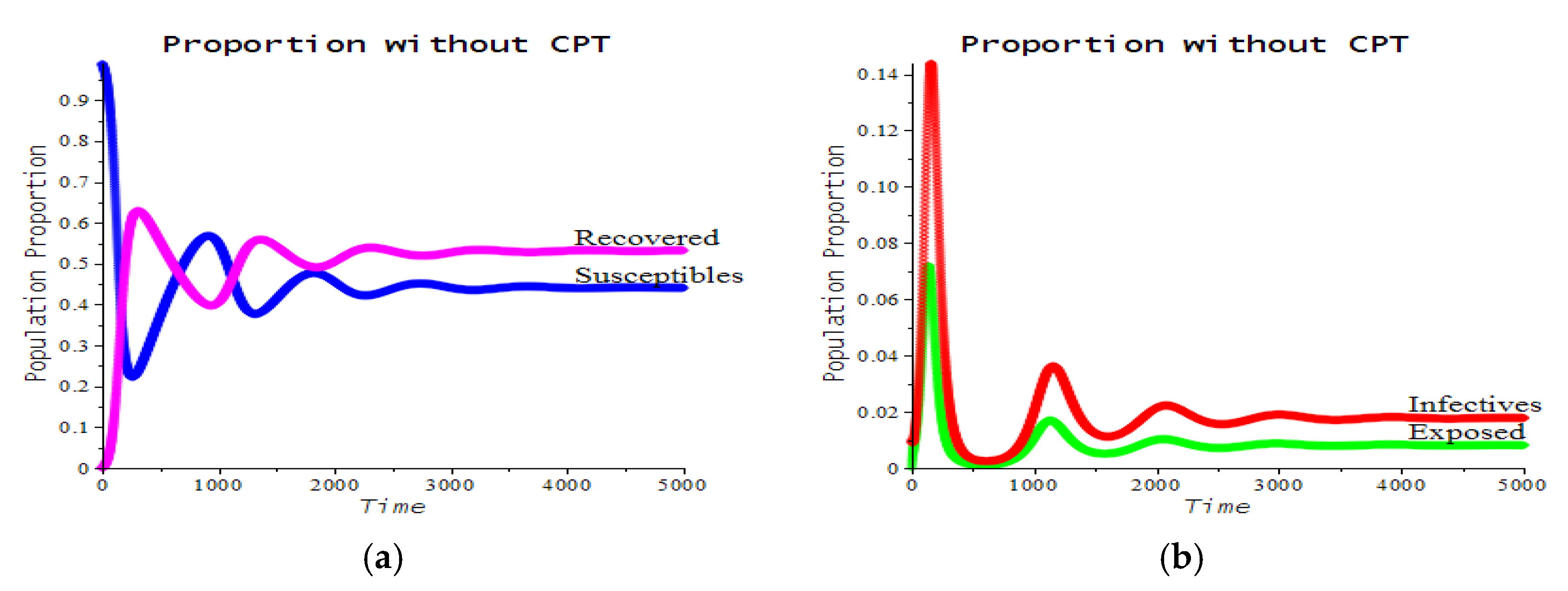
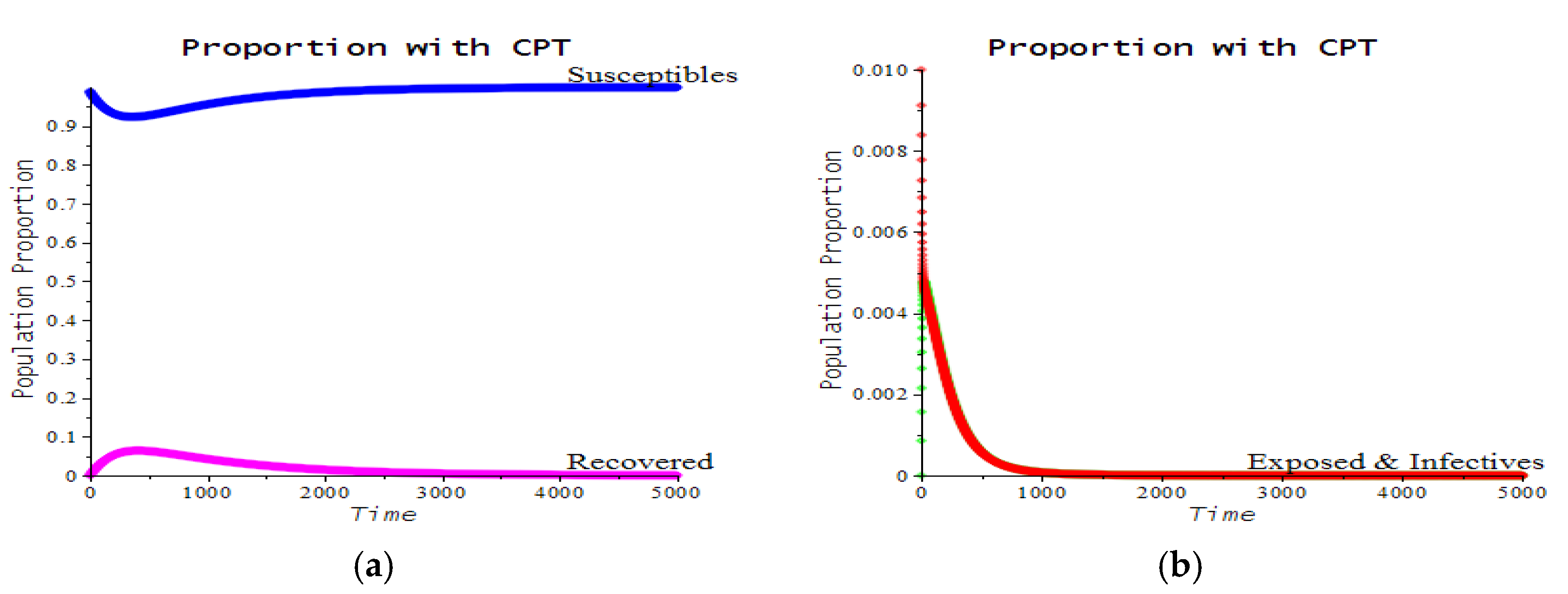
Figure 2 shows a graph of the disease dynamics predicted by the SEIR model for specific parameters (written in the figure caption) with a high basic reproduction number (approximately 2.3). It suggests that, eventually, the disease will endemic to a certain level with a stable number of infectives (approximately 2% of the total population). Figure 3 shows the changes in the graph when CPT is utilized to cure patients. It shows that, for a relatively high rate of CPT intervention, it can reduce the basic reproduction number to the effective reproduction number as low as 0.97, which leads to a stable disease-free equilibrium.
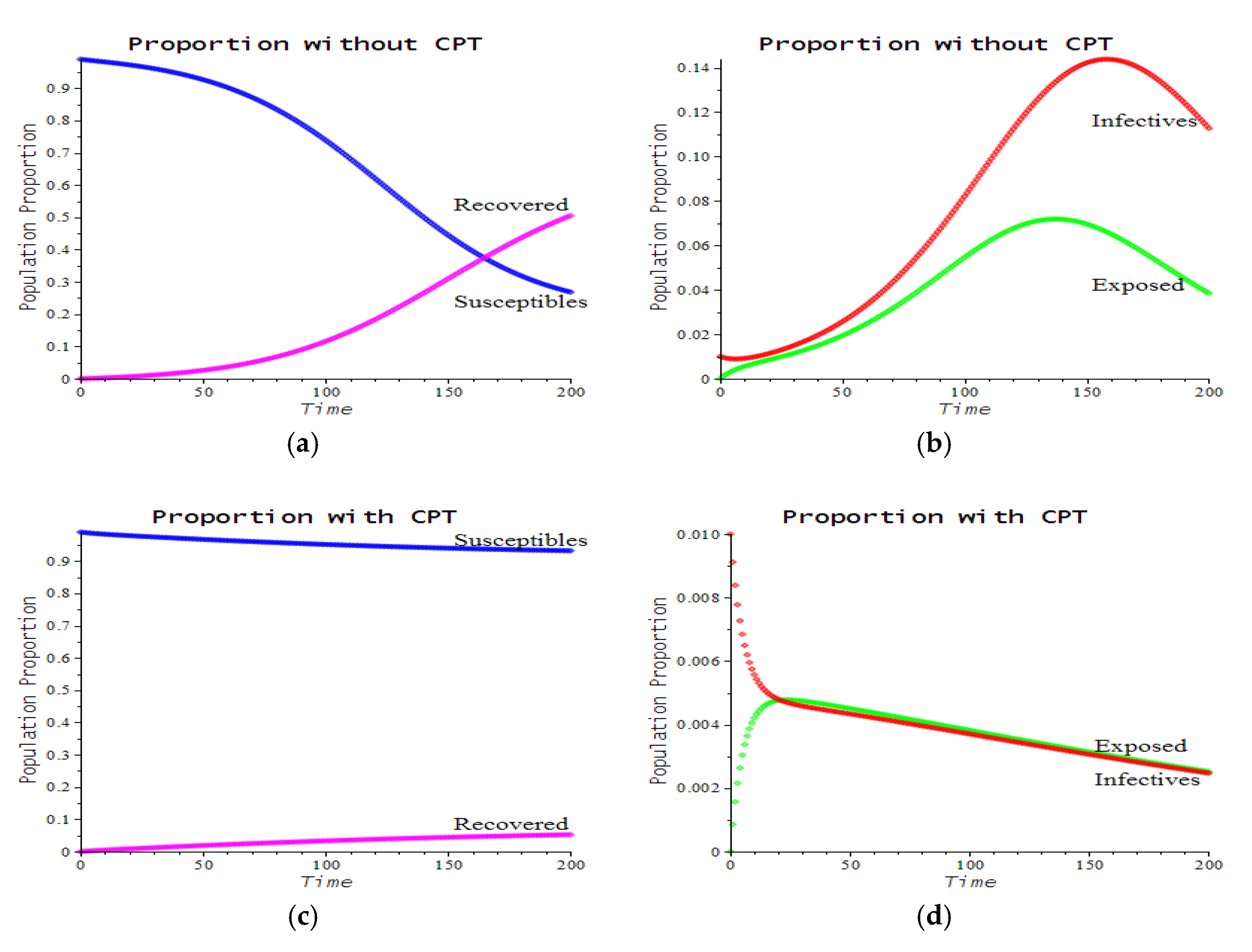
Figure 3 also suggests that early application of CPT significantly reduces the risk of disease outbreak. In the early transmission of COVID-19, this was clearly not the case, since COVID-19 is a new and emerging disease; hence, the availability of CP was almost null in the beginning. The figure also suggests a practical consequence of creating a convalescent plasma bank. Now, looking closer at the graph in Figure 2, during the first 200 time steps, we have the graph in Figure 4. It can be seen that there were already many recovered patients; hence, the availability of CP stock may be justified. Suppose that at time t = 200, the health authority begins to apply CPT as a curative method, then we have Figure 5, which shows that CPT significantly drove the disease cases down to zero, eventually. This is among the promising findings suggested by the SEIR model.
Figure 5 shows a graph of the SEIR model as in Figure 2, assuming that in the beginning (i.e., during the time interval (0,200)), the health authority takes the “do nothing” decision in controlling the disease (blue and red circles), and then, at time t = 200, begins to implement CPT with a relatively high rate of implementation (approximately half of the infectives are given CPT, proportional to the number of infectives with ε = 0.55). The black dots reveal that the intervention quickly pulls the number of infectives to zero (b) while, at the same time, pushes the number of susceptibles upward (a).
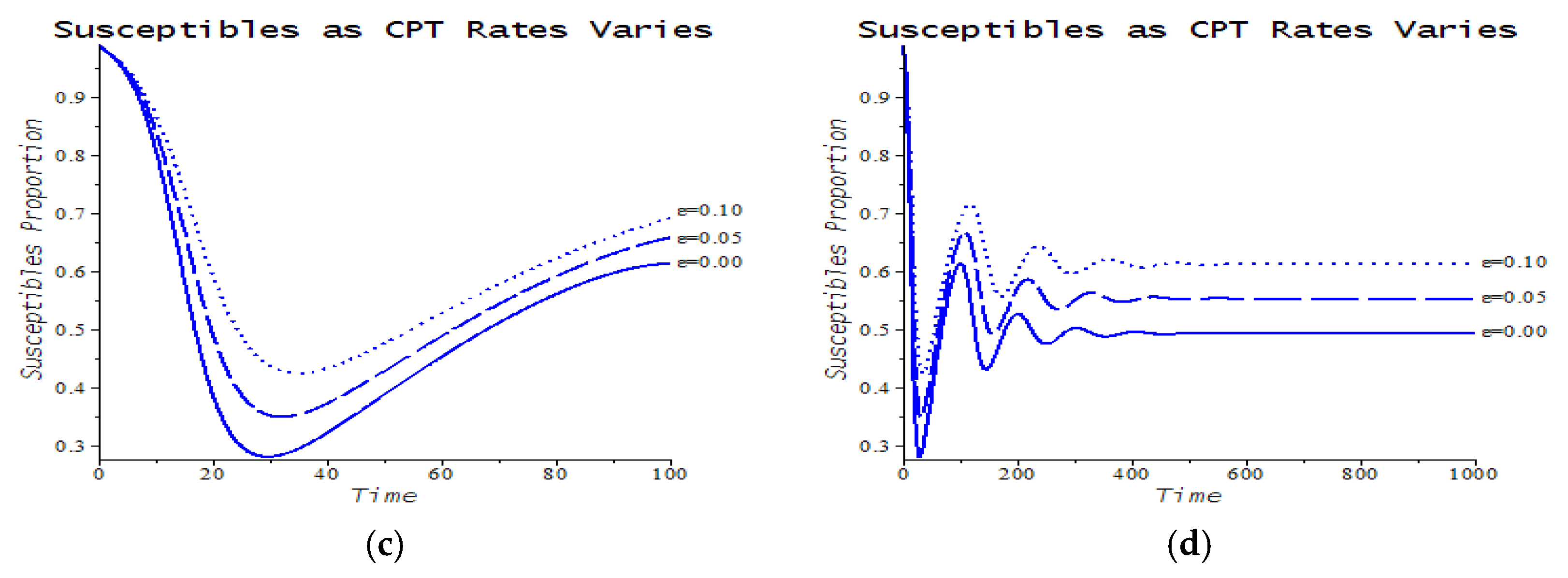
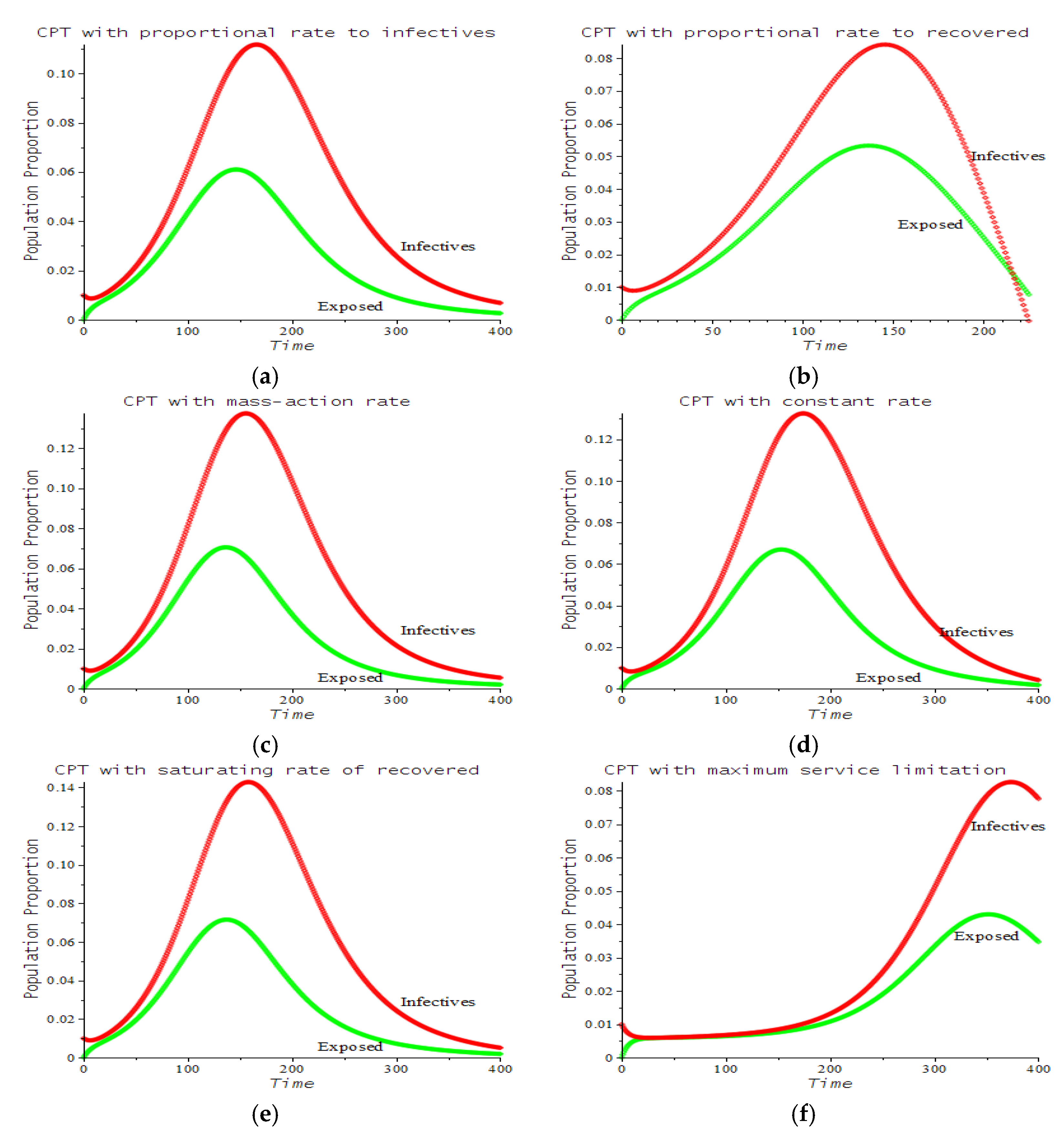
Figure 6 shows the effects of different rates of CPT on decreasing the number of infectives (hence, the height of the infective peak). Here, we assumed a scenario in which CPT is conducted with the rate proportional to the infectives (implicitly assuming an abundance of CP bloods). Figure 7 shows the effect of different scenarios (see Table 1) on the decrease in the infective numbers over time. All of the figures assumed that there was no limit for the health authority to set CPT rates, except in Figure 7f, in which it was assumed that the maximum CPT rate was the Maxserv (response function number 6 in Table 2).
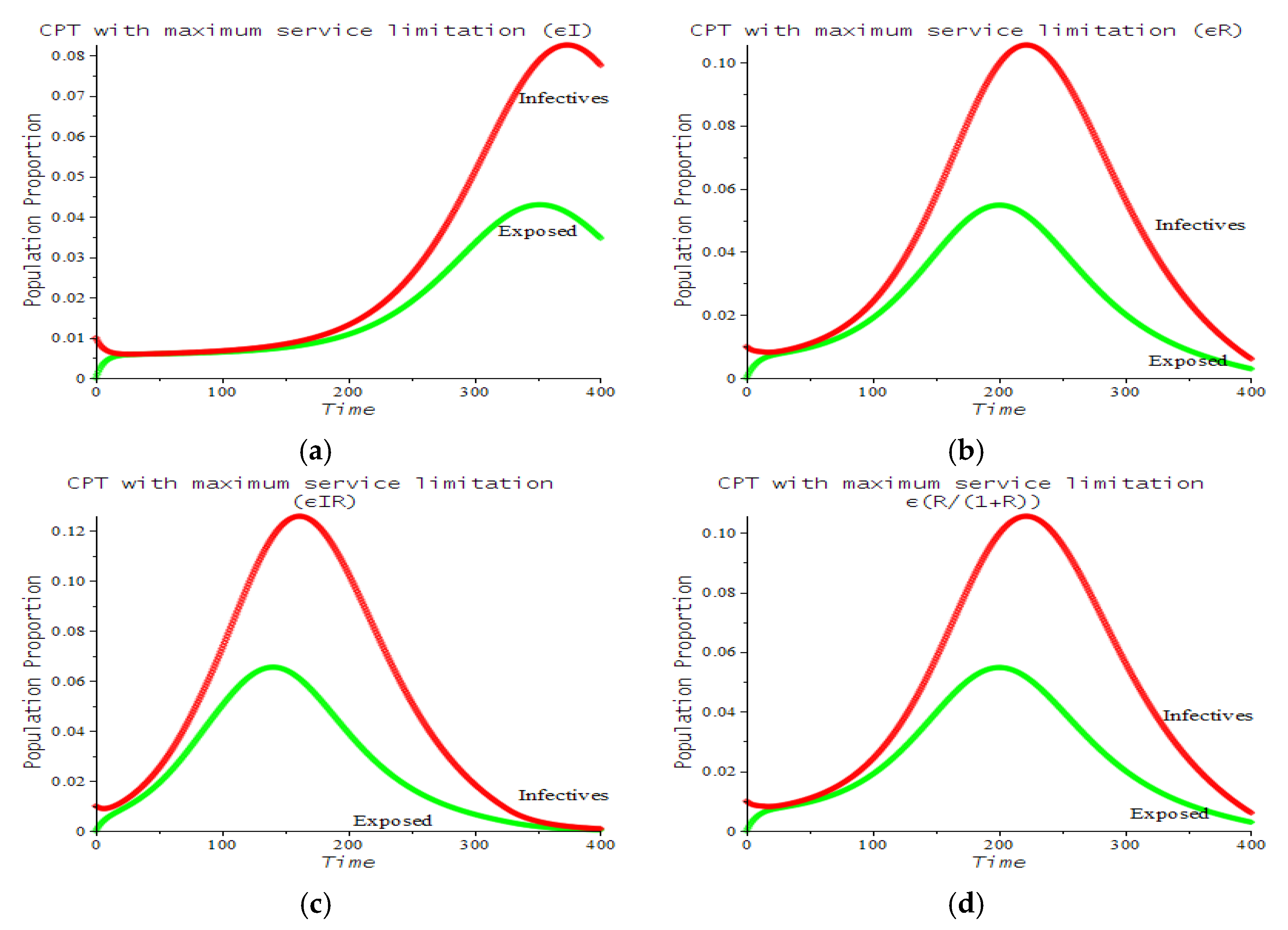
In Figure 7f, if the Maxserv is unbounded, then the result is the same as in Figure 3b, which is unlikely in reality. Figure 8 shows examples of the Maxserv graphs used in Figure 7. The effect of various Maxserv response functions on the numbers of infectives and the exposed population is shown in Figure 9.
In all of the numerical simulations above, we assumed that the effect of CPT was on increasing patient survival. The recent findings reported in [26] support the assumption we used in this paper. They carried out a meta-analytical approach to collect and analyze the daily survival data from all controlled studies that reported Kaplan–Meier survival plots. The authors showed that CPT contributes to improving the symptomatology and viral clearance. Furthermore, they pointed out that the aggregate Kaplan–Meier survival plot in their study revealed a good agreement pattern among all different studies in which CPT was generally associated with greater patient survival [26].
The historical evidence shows the promising results of applying the therapeutic treatment of CPT for critical patients infected by contagious diseases such as COVID-19. A more recent study provided strong evidence that if the convalescent plasma is transfused into patients within three days of the onset of illness, a 41% lower risk of death compared to patients transfused four or more days after onset of illness is demonstrated [26,27]. This remarkable result highlights an important role for the timely use of convalescent plasma transfusion. We discussed all such situations in terms of mathematical modeling with real data collected from a secondary source in the numerical analysis.
In this research, a standard analytical evaluation, from proving the existence of equilibria, their local stability, and their relationships with the reproduction numbers, was only carried out for the model with the response function for the CPT rate proportional to the number of infected class. The numerical simulations showed the consistency of other forms of the response functions with the findings in real phenomena such as reported in [26,27]. However, to obtain more prudent results, it is necessary to undertake a complete mathematical analysis of all proposed response functions that will presumably provide more in-depth insight and better implementation. Well-posedness of solutions and the threshold criteria for the global stability of equilibria should certainly be sought [28]. On the contrary, the numerical solutions presented in this paper were obtained by the RK45, although according to the current findings [29,30], there is a better scheme to produce a dynamically consistent numerical solution. Other future research could focus on the application of optimal control theory for disease prevention and control based on different nonlinear response functions for the therapeutic rate of CPT. In particular, a study concentrating on applying a wider class of control variables to formulate an optimal control problem in order to find better control and preventive strategies in CPT implementation would be beneficial as found in [31].

4. Conclusions

We presented a continuous SEIR epidemic model considering the effect of an intervention using convalescent plasma transfusion (CPT) to the infected class. We analyzed the model using the standard procedure and found the trivial and non-trivial equilibrium points of the system including their stability and relation to the basic reproduction number. In general, the effect of the application of CPT on the individual level resulted in a shorter time of infection and a higher survival rate for infected individuals that received CPT. Furthermore, we showed that at the population level, it could also decrease the peak of the outbreak as well as the length of the epidemic period. In this case, the decrease in the infection peak indicated the good effect of the use of CPT, which may eventually decrease the burden of COVID-19 transmission. The model presented here is still simple in terms of biological and epidemiological complexity; hence, further refinement of the model is still needed to obtain a more realistic model and a more accurate prediction.
In this paper, we proposed various functional forms/numerical responses that could be used to model the CPT rate, but not all were evaluated analytically. These numerical responses can be considered as a parametric viewpoint of control strategy. Hence, analytical investigation regarding the use of these various functional forms is also worthy to explore the robustness of the results presented here and to generate some possible epidemiological precautions not explored in the current paper. The model in this paper also only assumed a single strain or variant. In reality, viruses are always changing and mutating, and this could cause a new strain or variant. How would the results here be affected by such phenomena? Another question important for future research involves finding optimal CPT strategies that minimize both the number of infections and the related costs of CPT implementation. Our future research will focus on the application of optimal control theory for disease prevention and control based on different nonlinear response functions for the therapeutic rate of CPT. In particular, we will concentrate on applying a wider class of control variables to formulate an optimal control problem in order to find better control and preventive strategies for implementation of CPT.

Author Contributions

Conceptualization, H.H. and A.K.S.; methodology, H.H., A.K.S. and M.H.A.B.; software, A.K.S.; validation, H.H. and R.R.; formal analysis, A.K.S.; investigation, R.R.; resources, R.R.; data curation, R.R.; writing—original draft preparation, H.H.; writing—review and editing, H.H. and M.H.A.B.; visualization, A.K.S.; supervision, A.K.S.; project administration, H.H.; funding acquisition, H.H. All authors have read and agreed to the published version of the manuscript.

Funding

This research was funded by the Indonesian Government through the scheme “Penelitian Kompetitif Nasional dan Penelitian Dasar”, contract number 1207/UN6.3.1/PT.00/2021.

Institutional Review Board Statement

Not applicable.

Conflicts of Interest

The authors declare no conflict of interest.

References

  1. WHO. WHO Announces COVID-19 Outbreak a Pandemic. Available online: https://www.euro.who.int/en/health-topics/health-emergencies/coronavirus-covid-19/news/news/2020/3/who-announces-covid-19-outbreak-a-pandemic (accessed on 10 September 2021).
  2. Worldometer 2020. Available online: https://www.worldometers.info/coronavirus/ (accessed on 1 November 2021).
  3. FDA. FDA Issues Emergency Use Authorization for Convalescent Plasma as Potential Promising COVID–19 Treatment, Another Achievement in Administration’s Fight against Pandemic. Available online: https://www.fda.gov/news-events/press-announcements/fda-issues-emergency-use-authorization-convalescent-plasma-potential-promising-covid-19-treatment (accessed on 7 December 2020).
  4. Mayo Clinic. Patient Care & Health Information: Tests & Procedures: Convalescent Plasma Therapy. Available online: https://www.mayoclinic.org/tests-procedures/convalescent-plasma-therapy/about/pac-20486440 (accessed on 7 December 2020).
  5. Klassen, S.A.; Senefeld, J.W.; Johnson, P.W.; Carter, R.E.; Wiggins, C.C.; Shoham, S.; Grossman, B.J.; Henderson, J.P.; Musser, J.; Salazar, E.; et al. The Effect of Convalescent Plasma Therapy on Mortality among Patients With COVID-19: Systematic Review and Meta-Analysis. Mayo Clin. Proc. 2021, 96, 1262–1275. Available online: https://www.mayoclinicproceedings.org/article/S0025-6196(21)00140-3/fulltext (accessed on 18 October 2021). [CrossRef] [PubMed]
  6. CNN Indonesia. 4 RS di RI Yang Mulai Terapi Plasma Darah Obati Pasien Corona (in Bahasa Indonesia). Available online: https://www.cnnindonesia.com/teknologi/20200908163921-199-544140/4-rs-di-ri-yang-mulai-terapi-plasma-darah-obati-pasien-corona (accessed on 7 December 2020).
  7. Lewin, E. Australian COVID-19 Trials Add Convalescent Plasma as a Treatment. NewGP 30 July 2020. Available online: https://www1.racgp.org.au/newsgp/clinical/australian-covid-19-trials-add-convalescent-plasma (accessed on 1 November 2021).
  8. Agarwal, A.; Mukherjee, A.; Kumar, G.; Chatterjee, P.; Bhatnagar, T.; Malhotra, P.; on behalf of the PLACID Trial Collaborators. Convalescent plasma in the management of moderate COVID-19 in adults in India: Open label phase II multicentre randomised controlled trial (PLACID Trial). BMJ 2020, 371, 371. [Google Scholar] [CrossRef] [PubMed]
  9. Garroud, O.; Heshmati, F.; Pozzetto, B.; Lefrere, F.; Girot, R.; Saillol, A. Plasma therapy against infectious pathogens, as of yesterday, today and tomorrow. Transfus. Clin. Biol. 2016, 23, 39–44. [Google Scholar] [CrossRef] [PubMed]
  10. Marson, P.; Cozza, A.; De Silvestro, G. The true historical origin of convalescent plasma therapy. Transfus. Apheresis Sci. 2020, 59, 102847. [Google Scholar] [CrossRef] [PubMed]
  11. Cao, H.; Shi, Y. Convalescent plasma: Possible therapy for novel coronavirus disease 2019. Transfusion 2020, 60, 1078–1083. [Google Scholar] [CrossRef] [PubMed]
  12. Salazar, E.; Perez, K.K.; Ashraf, M.; Chen, J.; Castillo, B.; Christensen, P.A.; Eubank, T.; Bernard, D.W.; Eagar, T.N.; Long, S.W.; et al. Treatment of Coronavirus Disease 2019 (COVID-19) patients with convalescent plasma. Amer. J. Pathol. 2020, 190, 1680–1690. [Google Scholar] [CrossRef] [PubMed]
  13. Salazar, E.; Christensen, P.A.; Graviss, E.A.; Nguyen, D.T.; Castillo, B.; Chen, J.; Lopez, B.V.; Eagar, T.N.; Yi, X.; Zhao, P.; et al. Significantly decreased mortality in a large cohort of Coronavirus Disease 2019 (COVID-19) patients transfused early with convalescent plasma containing high-titer Anti-Severe Acute Respiratory Syndrome Coronavirus 2 (SARS-CoV-2) spike protein IgG. Am. J. Pathol. 2020, 191, 90–107. [Google Scholar] [CrossRef] [PubMed]
  14. Peng, H.T.; Rhind, S.G.; Beckett, A. Convalescent plasma for the prevention and treatment of COVID-19: A systematic review and quantitative analysis. JMIR Public Health Surveill. 2021, 7, e25500. [Google Scholar] [CrossRef] [PubMed]
  15. Huo, X.; Sun, X.; Bragazzi, N.L.; Wu, J. Effectiveness and feasibility of convalescent blood transfusion to reduce COVID-19 fatality ratio. Roy. Soc. Open Sci. 2020, 8, 202248. [Google Scholar] [CrossRef] [PubMed]
  16. Supriatna, A.K.; Husniah, H. Can convalescent plasma transfusion reduce the COVID-19 transmission? In Proceedings of the 2nd African International Conference on Industrial Engineering and Operations Management, IEOM, Harare, Zimbabwe, 7–10 December 2020; pp. 3116–3124. [Google Scholar]
  17. Nykamp, D.Q.; Morrissey, D.P. A Discrete SIR Infectious Disease Model. From Math Insight. Available online: http://mathinsight.org/discrete_sir_infectious_disease_model (accessed on 30 September 2021).
  18. Switkes, J. A Modified Discrete SIR Model. Coll. Math. J. 2003, 3, 399–402. [Google Scholar] [CrossRef] [Green Version]
  19. Diekmann, O.; Heesterbeek, J.A.P. Mathematical Epidemiology of Infectious Diseases: Model Building, Analysis and Interpretation, 1st ed.; Wiley: New York, NY, USA, 2000. [Google Scholar]
  20. Anderson, R.M.; May, R.M.; Anderson, B. Infectious Diseases of Humans: Dynamics and Control, Revised ed.; Oxford University Press: London, UK, 1992. [Google Scholar]
  21. Brauer, F.; van den Driessche, P.; Wu, J. Mathematical Epidemiology; Springer: Berlin/Heidelberg, Germany, 2008. [Google Scholar]
  22. Diekmann, O.; Heesterbeek, J.A.P.; Metz, J.A.J. On the definition and the computation of the basic reproduction ratio R 0 in models for infectious diseases in heterogeneous populations. J. Math. Biol. 1990, 28, 365–382. [Google Scholar] [CrossRef] [PubMed] [Green Version]
  23. Diekmann, O.; Heesterbeek, J.A.P.; Roberts, M.G. The construction of next-generation matrices for compartmental epidemic models. J. R. Soc. Interface 2010, 7, 873–885. [Google Scholar] [CrossRef] [PubMed] [Green Version]
  24. Van den Driessche, P.; Watmough, J. Reproduction numbers and sub-threshold endemic equilibria for compartmental models of disease transmission. Math Biosci. 2002, 180, 29–48. [Google Scholar] [CrossRef]
  25. Zhao, X.Q. The Theory of Basic Reproduction Ratios. In Dynamical Systems in Population Biology; Springer Nature Switzerland AG: Cham, Switzerland, 2003. [Google Scholar] [CrossRef]
  26. Klassen, S.A.; Senefeld, J.W.; Senese, K.A.; Johnson, P.W.; Wiggins, C.C.; Baker, S.E.; van Helmond, N.; Bruno, K.A.; Pirofski, L.; Shoham, S.; et al. Convalescent Plasma Therapy for COVID-19: A Graphical Mosaic of the Worldwide Evidence. Front. Med. 2021, 8, 684151. [Google Scholar] [CrossRef] [PubMed]
  27. Liu, S.T.H.; Lin, H.M.; Baine, I.; Wajnberg, A.; Gumprecht, J.P.; Rahman, F.; Rodriguez, D.; Tandon, P.; Bassily-Marcus, A.; Bander, J.; et al. Convalescent plasma treatment of severe COVID-19: A propensity score–matched control study. Nat. Med. 2020, 26, 1708–1713. [Google Scholar] [CrossRef] [PubMed]
  28. Chen, W.; Wu, W.X.; Teng, Z.D. Complete dynamics in a nonlocal dispersal two-strain SIV epidemic model with vaccinations and latent delays. Appl. Comput. Math. 2020, 19, 360–391. [Google Scholar]
  29. Khalsaraei, M.M.; Shokri, A.; Ramos, H.; Heydari, S. A positive and elementary stable nonstandard explicit scheme for a mathematical model of the influenza disease. Math. Comput. Simul. 2021, 182, 397–410. [Google Scholar] [CrossRef]
  30. Shokri, A.; Khalsaraei, M.M.; Molayi, M. Dynamically consistent NSFD methods for predator prey system. J. Appl. Comput. Mech. 2021, 7, 1565–1574. [Google Scholar] [CrossRef]
  31. Biswas, M.H.A.; Paiva, L.T.; de Pinho, M. A SEIR model for control of infectious diseases with constraints. Math. Biosci. Eng. 2014, 11, 761–784. [Google Scholar] [CrossRef]
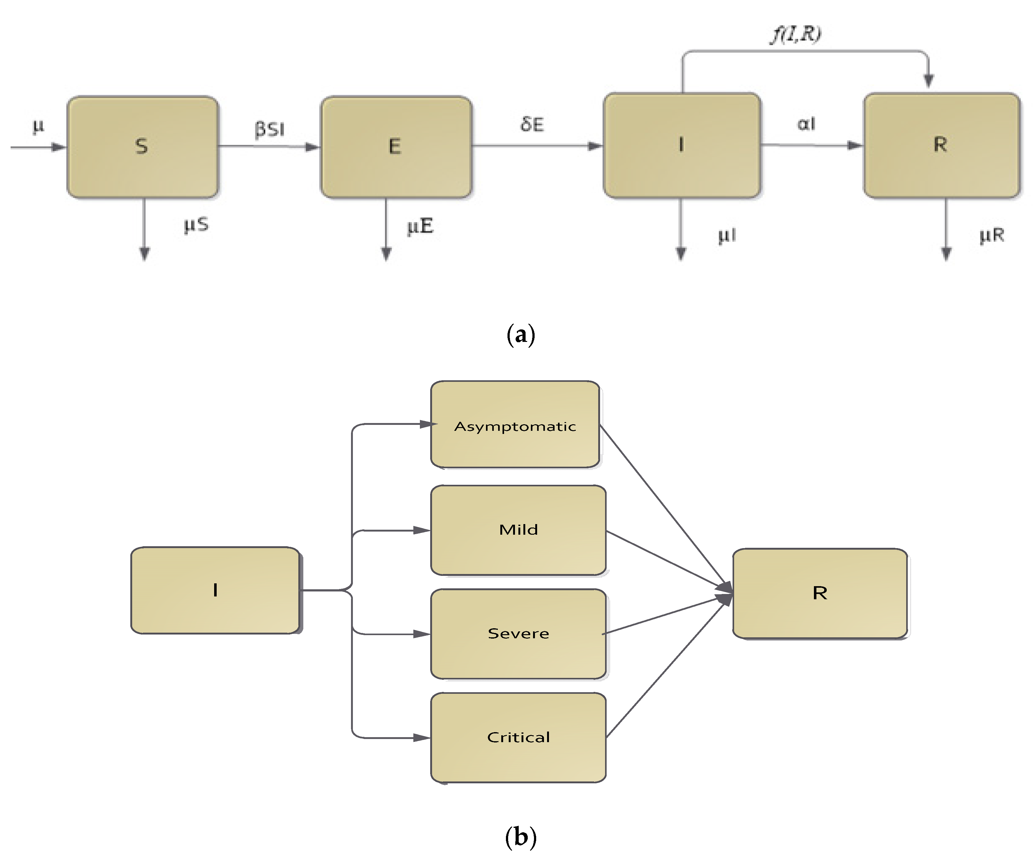
Figure 1. Progression diagram of SEIR transmission with CPT effect f(I(t),R(t)) (a) and four possible severity levels of COVID-19 infected patients (b).
Mathematics 09 02857 g001
Figure 2. A graph of the SEIR model without CPT showing the susceptible and recovered classes (a) and the exposed and infective classes (b). The SEIR parameters were μ = 1/75, β = 0.95, δ = 0.90, and α = 0.40, with initial values of S0 = 0.99, E0 = 0, I0 = 0.01, and R0 = 0. The resulting equilibrium was approximately S = 44%, E = 1%, I = 2%, and R = 53% with the basic reproduction number 0 = 2.265 .
Mathematics 09 02857 g002
Figure 3. A graph of the SEIR model with CPT, showing the susceptible and recovered classes (a) and the exposed and infective classes (b). The SEIR parameters were μ = 1/75, β = 0.95, δ = 0.90, and α = 0.40, with initial values of S0 = 0.99, E0 = 0, I0 = 0.01, and R0 = 0. The CPT rate was assumed to be ε = 0.55. The resulting equilibrium was approximately S = 99%, R = 0.05%, and the remaining E and I were nearly zero. In this case, the resulting effective reproduction number was 0 = 0.97 (less than 1).
Mathematics 09 02857 g003
Figure 4. A graph of the SEIR model without CPT (top figures) showing the susceptible and recovered classes (a) and the exposed and infective classes (b) as in Figure 2 but with a shorter time horizon. (c,d) With CPT. The bottom figures show similar graphs for the SEIR model with CPT as in Figure 3 but with a shorter time horizon.
Mathematics 09 02857 g004
Figure 5. Graphs of the SEIR model assuming the “do nothing” decision during the time interval (0,200), followed by the implementation of CPT with the rate proportional to the number of infectives. The graph in (a) shows the dynamics of the susceptibles, while the graph in (b) shows the dynamics of the infectives.
Mathematics 09 02857 g005
Figure 6. Graphs showing the effects of different rates of CPT on decreasing the number of infectives (i.e., lowering the height of the infective peaks) (a,b) and, consequently, increasing the number of remaining susceptibles (c,d). The other parameters were the same as in Figure 2.
Mathematics 09 02857 g006aMathematics 09 02857 g006b
Figure 7. Plots of the effect of various CPT scenarios on the dynamics of the infective (red) and exposed (green) classes, with the assumption that the CPT intervention was carried out from the beginning of the pandemic. The scenarios and parameters were the same as in Table 2. The response functions and the parameters in the response functions for the graphs in (af) are presented in Table 2. See also Figure 2 as the reference for the other epidemiological parameters. Note that if Maxserv is unbounded, then the result is the same as Figure 3b.
Mathematics 09 02857 g007
Figure 8. The graph in (a) shows a plot the of mass action term of ε I ( t ) R ( t ) in Figure 7c. The graph in (b) shows a plot of the numerical response min ( ε I ( t ) R ( t ) , Maxserv ) used in Figure 7f with ε = 1 and Maxserv = 0.01.
Mathematics 09 02857 g008
Figure 9. Plots of the effect of various Maxserv CPT scenarios on the dynamics of infective (red) and exposed (green) classes, with the assumption that the CPT intervention is conducted from the beginning of the pandemic. The scenarios and parameters for the graphs in (ad) are as in Table 2.
Mathematics 09 02857 g009
Table 1. Different possible scenarios of CPT implementation.
NumberCPT ScenarioNumerical Response f ( I ( t ) , R ( t ) )
1Proportional rate to infectives ε I ( t )
2Proportional rate to recovered ε R ( t )
3Mass action rate (Lotka–Volterra) ε I ( t ) R ( t )
4Constant rate ε
5Saturating rate (Michaelis–Menten) ε R ( t ) r + R ( t )
6Maximum service limitation min ( ε I ( t ) , Maxserv )
7Maximum service limitation min ( ε R ( t ) , Maxserv )
8Maximum service limitation min ( ε I ( t ) R ( t ) , Maxserv )
9Maximum service limitation min ( ε R ( t ) r + R ( t ) , Maxserv )
Maxserv is the maximum rate of CPT intervention that a health authority could afford.
Table 2. Parameter values used for different scenarios of CPT implementation.
NumberCPT ScenarioNumerical Response
f ( I ( t ) , R ( t ) )
Used in the Figures Parameter Values in the Figures
1Proportional rate to infectives ε I ( t ) 7.a ε = 0.05
2Proportional rate to recovered ε R ( t ) 7.b ε = 0.05
3Mass action rate (Lotka–Volterra) ε I ( t ) R ( t ) 7.c ε = 0.05
4Constant rate ε 7.d ε = 0.001
5Saturating rate (Michaelis–Menten) ε R ( t ) r + R ( t ) 7.e ε = 0.001 ,   r = 0
6Maximum service limitation min ( ε I ( t ) , Maxserv ) 7.f, 9.a ε = 0.55 , Maxserv = 0.0028
7Maximum service limitation min ( ε R ( t ) , Maxserv ) 9.b ε = 0.55 , Maxserv = 0.0028
8Maximum service limitation min ( ε I ( t ) R ( t ) , Maxserv ) 9.c ε = 0.55 , Maxserv = 0.0028
9Maximum service limitation min ( ε R ( t ) r + R ( t ) , Maxserv ) 9.d ε = 0.55 , Maxserv = 0.0028
Publisher’s Note: MDPI stays neutral with regard to jurisdictional claims in published maps and institutional affiliations.