Reachability and Observability of Positive Linear Electrical Circuits Systems Described by Generalized Fractional Derivatives

Abstract

Positive linear electrical circuits systems described by generalized fractional derivatives are studied in this paper. We mainly focus on the reachability and observability of linear electrical circuits systems. Firstly, generalized fractional derivatives and $\rho$-Laplace transform of f is presented and some preliminary results are provided. Secondly, the positivity of linear electrical circuits systems described by generalized fractional derivatives is investigated and conditions for checking positivity of the systems are derived. Thirdly, reachability and observability of the generalized fractional derivatives systems are studied, in which the $\rho$-Laplace transform of a Mittag-Leffler function plays an important role. At the end of the paper, illustrative electrical circuits systems are presented, and conclusions of the paper are presented.

1. Introduction

Fractional differential equations play an important role in the analysis and modeling of various processes. Many classical methods, such as perturbation method [1], Fourier transform and Merlin transform, have important applications in fractional calculus. Fractional calculus has many new diffusion processes in physics [2,3,4]. There are many types of fractional derivatives in fractional calculus, see [5,6,7,8,9,10,11] for details. For the basic principles of fractional calculus and its most interesting applications, see [12,13,14,15,16,17,18]. In recent years, fractional calculus has become a useful and promising tool in modeling and analyzing different dynamic behavior processes. Fractional calculus system has attracted more and more scholars’ attention since its wide application value in the field of science and engineering.

Fractional derivative has more advantages than classical derivative. The first advantage is that the fractional derivative takes into account memory. Memory effect is a basic property of differential equations. This explains the application of fractional derivative in differential equation modeling [14,16]. Another advantage is that the fractional derivative produces many diffusion processes [4]. Due to these advantages, fractional derivative also has many applications in electronics [15,19,20].

The new mathematical model appears with the emergence of fractional derivative. In recent years, researchers began to apply fractional derivatives to describe electrical circuit systems. Many types of fractional electrical circuits have been introduced recently in the literature, see [14,15,19,20] and fractional RL (Resistor-Inductor) and RC (Resistor-Capacitance) circuit modeling in [11,18,21,22,23]. Many studies on the properties of fractional electrical circuit system will use numerical solutions and analytical solutions., because it is an important way to study properties of circuits systems. Reference [18] studies the analytical and numerical solutions of fractional RL and RC circuits using Atangana-Baleanu derivative and bi-order derivative. Reference [21] studies the solutions of fractional electrical RL, LC (Inductor-Capacitance) and RC electrical circuit systems described by Mittag-Leffler fractional derivatives. Fractional RL and LC electrical circuits systems are studied in reference [22]. They also compared the fractional electrical circuit systems with the traditional electrical circuit systems.

In the literature of fractional electrical circuits systems, many studies mainly focus on performance properties of systems, such as stability [11,23,24,25,26,27,28,29,30,31,32]. In [27,28], the asymptotic stability of integer and fractional positive continuous-time linear system with delays is studied, respectively. The necessary and sufficient conditions for the asymptotic stability of integer and fractional positive linear system with delays are given, and it is proved that the asymptotic stability integer and fractional of the systems is independent of delays. By comparison, it can be found that the asymptotic stability conditions and checking methods of integer and fractional positive linear systems with delays are similar. In recent years, generalized fractional derivative has been widely used in stability analysis. For more details, see [6,33,34]. In [29], several stabilities of fractional differential equations described by Caputo type generalized fractional derivatives are studied. In this paper, a new concept of stability, fractional input stability is introduced. Thus, it provides a new idea and method for the stability analysis of fractional differential equations described by generalized fractional derivatives. In [32], the stability of RLC (Resistor-Inductor-Capacitance) electrical circuits described by Caputo-Liouville generalized fractional derivatives is studied. The local asymptotic stability and global asymptotic stability of trivial equilibrium are analyzed. The results of this paper are very valuable for the study of circuit stability. Of course, in addition to stability, electrical circuits systems have other performance properties [35,36,37], such as reachability and observability. In [37], fractional positive discrete-time linear systems are studied in the literature. The necessary and sufficient conditions of positivity, reachability and controllability are given. In [38], the reachability and observability of integer and fractional positive linear electrical circuits are studied.And it is found that the reachability and observability of integer and fractional positive linear electrical circuits are invariant. At this time, reference [39] further extends the result of [38] to positive linear electrical circuits with delays. In [39], the electrical circuit systems are extended to positive linear electrical circuits with delays, and it is found that the reachability and observability of integer and fractional positive linear electrical circuits with delays are similar. Many scholars have studied the properties of electrical circuits described by generalized fractional derivatives and positive linear electrical circuit systems. In this paper, generalized fractional derivatives are applied to positive linear electrical circuit systems.

The generalized fractional derivative units the Riemann-Liouville fractional derivative and Hadamard fractional derivative into a unified form in that it is mediated by an additional fractional parameter, which is more general than the ordinary classical fractional derivative. By observing, we can find that when $\alpha$ is fixed, the smaller the parameter $\rho$ is, the greater the initial slope of the described circuit trajectory is, and the more realistic the described trajectory is. Contributions of this paper are listed below:

(1) We present the positivity of linear electrical circuits systems described by generalized fractional derivatives and obtained conditions for checking positivity of the systems. Also we investigate the checking method of reachability and observability of the generalized fractional derivatives studied.

(2) In references [23,29], the $\rho$-Laplace transform was performed on the Mittag-Leffler function with a constant $\lambda$, but we are extended to the Mittag-Leffler function with matrix A, and the corresponding form of $\rho$-Laplace transform is obtained.

(3) We investigate the effect of the parameter $\rho$ on the electrical circuits systems. Since the generalized fractional derivative involves parameters, which is more general than the classical fractional derivative. Therefore, we studied the electrical circuits systems by illustrative examples when the fixed order $\alpha$ is unchanged, We let the parameter $\rho$ take different values to observe how the parameter $\rho$ affects the change of state trajectories.

The remainder of the paper is organized as follows. In Section 2, generalized fractional integrals, derivatives and $\rho$-Laplace transform are reviewed and some new results are given. Positive linear electrical circuits systems described by generalized fractional derivatives are presented in Section 3. In Section 4, reachability of positive linear electrical circuits systems described by generalized fractional derivatives are investigated. Observability of positive linear electrical circuits systems described by generalized fractional derivatives are investigated in Section 5. The illustrative electrical circuits are presented in Section 6. Concluding remarks are given in Section 7.

The following notation will be used in this paper. R is a set of real numbers, $R^{n\times m}$ is a set of $n\times m$ dimensional real matrix, $R_{+}^{n\times m}$ is a set of $n\times m$ dimensional real matrix with nonnegative entries and $R_{+}^n=R_{+}^{n\times 1}$, $M_n$ is a set of $n\times n$ Metzler matrix (real matrix with nonnegative off-diagonal entries).

2. Generalized Fractional Integrals, Derivatives and $\rho$-Laplace Transform

For the knowledge of classical fractional calculus, we refer to references [7,13], in which there are many types of fractional integrals and derivatives. In this paper, we consider the following forms of generalized fractional integrals:

$$({{}_{a}I}^{\alpha ,\rho }f)(x)=\frac{1}{\mathsf{\Gamma }(\alpha )}{\int }_a^x{(\frac{x^{\rho }-t^{\rho }}{\rho })}^{\alpha -1}f(t)\frac{dt}{t^{1-\rho }}$$

(1)

and

$$(I_b^{\alpha ,\rho }f)(x)=\frac{1}{\mathsf{\Gamma }(\alpha )}{\int }_x^b{(\frac{t^{\rho }-x^{\rho }}{\rho })}^{\alpha -1}f(t)\frac{dt}{t^{1-\rho }}.$$

(2)

where $\alpha$ is the order, $\rho$ is an additional fractional parameter, and integrals (1) and (2) are left generalized fractional integral and right generalized fractional integral, respectively. We can find that when $\rho =1$, the integrals (1) and (2) become Riemann-Liouville fractional integrals. See [13] for details. When the limit is $\rho \to 0$, the integrals (1) and (2) will become Hadamard fractional integrals defined in [7].

The generalized fractional derivatives defined by [6] for order $\alpha >0$ are as follows:

$$({{}_{a}D}^{\alpha ,\rho }f)(x)={\gamma }^n({{}_{a}I}^{n-\alpha ,\rho }f)(x)=\frac{{\gamma }^n}{\mathsf{\Gamma }(n-\alpha )}{\int }_a^x{(\frac{x^{\rho }-t^{\rho }}{\rho })}^{n-\alpha -1}f(t)\frac{dt}{t^{1-\rho }}$$

(3)

and

$$(D_b^{\alpha ,\rho }f)(x)=(-{\gamma }^n)({{}_{a}I}^{n-\alpha ,\rho }f)(x)=\frac{-{\gamma }^n}{\mathsf{\Gamma }(\alpha )}{\int }_x^b{(\frac{t^{\rho }-x^{\rho }}{\rho })}^{n-\alpha -1}f(t)\frac{dt}{t^{1-\rho }}$$

(4)

where fractional parameter $\rho >0$, $n=\lfloor \alpha \rfloor +1$ and $\gamma =x^{1-\rho }\frac{d}{dx}$.

Derivatives (3) and (4) are left and right generalized fractional derivatives, respectively. We can find that when $\rho =1$, the derivatives (3) and (4) become Riemann-Liouville fractional derivatives. See [13] for details. When the limit is $\rho \to 0$, the derivatives (3) and (4) will become Hadamard fractional derivatives defined in [7].

The reason we study the generalized fractional derivative is that it generalizes the Riemann-Liouville fractional derivative and Hadamard fractional derivative into one form. When the parameters are fixed at different values or take limits, the above derivative is generated as a special case [6]. The generalized fractional derivative is more general than the ordinary classical fractional derivative.

Let’s recall some details of the $\rho$-Laplace transform and its basic concepts, which plays an important role in the next research.

Definition 1

([9]). The ρ-Laplace transform of a continuous function $f:[0,\infty )\to R$ is defined by

$${\mathcal{L}}_{\rho }\{f(x)\}(s)={\int }_0^{\infty }{e}^{-s\frac{x^{\rho }}{\rho }}f(x)\frac{dx}{x^{1-\rho }},\rho >0,$$

(5)

The integral is valid for all values of s.

Theorem 1

([7]). If the ρ-Laplace transform of a continuous function $f:[0,\infty )\to R$ exists, the following relationship holds

$${\mathcal{L}}_{\rho }\{f(x)\}(s)=\mathcal{L}\{f({(\rho x)}^{\frac{1}{\rho }})\}(s),$$

(6)

where $\mathcal{L}\{f\}$ is the usual Laplace transform of f.

Theorem 2

([7]). If continuous function $f:[0,\infty )\to R$ has ρ-Laplace transform for $s>c_1$ and continuous function $g:[0,\infty )\to R$ has ρ-Laplace transform for $s>c_2$. Then, continuous function $af+bg$ has Laplace transform for any constants a and b, and has the following linear property

$${\mathcal{L}}_{\rho }\{af(x)+bg(x)\}(s)=a{\mathcal{L}}_{\rho }\{f(x)\}(s)+b{\mathcal{L}}_{\rho }\{g(x)\}(s),s>max\{c_1,c_2\}.$$

(7)

The reference [9] gave some $\rho$-Laplace transforms of elementary functions as shown below.

Theorem 3.

Suppose ${\mathcal{L}}_{\rho }\{·\}$ is the ρ-Laplace transform

$$\begin{array}{cc}\hfill (1)& {\mathcal{L}}_{\rho }\{1\}(s)=\frac{1}{s},s>0.\hfill \\ \hfill (2)& {\mathcal{L}}_{\rho }\{t^p\}(s)={\rho }^{\frac{p}{\rho }}\frac{\mathsf{\Gamma }(1+\frac{p}{\rho })}{s^{1+\frac{p}{\rho }}},p\in R,s>0.\hfill \\ \hfill (3)& {\mathcal{L}}_{\rho }\{e^{\lambda \frac{t^{\rho }}{\rho }}\}(s)=\frac{1}{s-\lambda },s>\lambda .\hfill \\ \hfill (4)& {\mathcal{L}}_{\rho }\{{(\frac{t^{\rho }}{\rho })}^{\alpha -1}{E}_{\alpha ,\alpha }(A{(\frac{t^{\rho }}{\rho })}^{\alpha })\}(s)={(s^{\alpha }I-A)}^{-1},A\in R^{n\times n},\rho (A)<s^{\alpha }\mathrm{and}\underset{n\to \infty }{lim}{(\frac{A}{s^{\alpha }})}^n=0,\hfill \end{array}$$

(8)

where ρ(A) is the spectral radius of the matrix A.

Proof. 

(1), (2) and (3) have been proved, please refer to [9] for details. Only (4) will be proved below

$${\mathcal{L}}_{\rho }\{{(\frac{t^{\rho }}{\rho })}^{\alpha -1}{E}_{\alpha ,\alpha }(A{(\frac{t^{\rho }}{\rho })}^{\alpha })\}(s)=\sum _{k=0}^{\infty }\frac{A^k}{\mathsf{\Gamma }(k\alpha +\alpha ){\rho }^{k\alpha +\alpha -1}}{\mathcal{L}}_{\rho }\{t^{k\alpha \rho +\alpha \rho -\rho }\}$$

(9)

From (2) we can get

$$\sum _{k=0}^{\infty }\frac{A^k}{\mathsf{\Gamma }(k\alpha +\alpha ){\rho }^{k\alpha +\alpha -1}}{\rho }^{k\alpha +\alpha -1}\frac{\mathsf{\Gamma }(k\alpha +\alpha )}{s^{k\alpha +\alpha }}=\frac{1}{s^{\alpha }}\sum _{k=0}^{\infty }{(\frac{A}{s^{\alpha }})}^k=\frac{1}{s^{\alpha }}(I+\frac{A}{s^{\alpha }}+\frac{A^2}{s^{2\alpha }}+\cdots ).$$

(10)

According to the famous Neumann series, we can know if $\underset{n\to \infty }{lim}{A}^n=0$, then $I-A$ is nonsingular and ${(I-A)}^{-1}=I+A+A^2+\cdots =\sum _{k=0}^{\infty }{A}^k$. In that case, here Equation (10) can be written in the following form

$$\frac{1}{s^{\alpha }}(I+\frac{A}{s^{\alpha }}+\frac{A^2}{s^{2\alpha }}+\cdots )=\frac{1}{s^{\alpha }}{(I-\frac{A}{s^{\alpha }})}^{-1}={(s^{\alpha }I-A)}^{-1}$$

(11)

where we can find an s and let $\underset{n\to \infty }{lim}{(\frac{A}{s^{\alpha }})}^n=0$, then $I-\frac{A}{s^{\alpha }}$ is nonsingular. Then

$${\mathcal{L}}_{\rho }\{{(\frac{t^{\rho }}{\rho })}^{\alpha -1}{E}_{\alpha ,\alpha }(A{(\frac{t^{\rho }}{\rho })}^{\alpha })\}(s)=\frac{1}{s^{\alpha }}{(I-\frac{A}{s^{\alpha }})}^{-1}={(s^{\alpha }I-A)}^{-1}$$

(12)

when $\underset{n\to \infty }{lim}{(\frac{A}{s^{\alpha }})}^n=0$, the above formula holds. □

Definition 2

([7]). Let fand g be two piecewise continuous functions on each interval $[0,T]$ and of exponential order. We define the ρ-convolution formula of functions f and g is

$$(f{\ast }_{\rho }g)(t)={\int }_0^{t}f({(t^{\rho }-{\tau }^{\rho })}^{\frac{1}{\rho }})g(\tau )\frac{d\tau }{{\tau }^{1-\rho }}$$

(13)

The following lemma gives the commutativity of $\rho$-convolution of two functions.

Lemma 1

([7]). Let fand g be two piecewise continuous functions on each interval $[0,T]$ and of exponential order. Then

$$f{\ast }_{\rho }g=g{\ast }_{\rho }f$$

(14)

Theorem 4

([7]). Let fand g be two piecewise continuous functions on each interval $[0,T]$ and of exponential order $e^{c\frac{t^{\rho }}{\rho }}$. Then

$${\mathcal{L}}_{\rho }\{f{\ast }_{\rho }g\}={\mathcal{L}}_{\rho }\{f\}{\mathcal{L}}_{\rho }\{g\}s>c.$$

(15)

The following theorem is the $\rho$-Laplace transformation of the left generalized fractional derivative starting from 0.

Theorem 5

([7]). Let $\alpha >0$ and $f\in A{C}_{\gamma }^n[0,a]$ for any $a>0$ and ${{}_{0}I}^{n-k-\alpha ,\rho }f$, $k=0,1,\dots ,n-1$ be of ρ-exponential order $e^{c\frac{t^{\rho }}{\rho }}$. Then

$${\mathcal{L}}_{\rho }\{({{}_{0}D}^{\alpha ,\rho }f)(t)\}(s)=s^{\alpha }{\mathcal{L}}_{\rho }\{f(t)\}-\sum _{k=0}^{n-1}{s}^{n-k-1}({{}_{0}I}^{n-k-\alpha ,\rho }f)(0),s>c.$$

(16)

3. Positive Linear Electrical Circuits Described by Generalized Fractional Derivatives

Consider the linear electrical circuit systems described by the left generalized fractional derivatives as the following system equation:

$$({{}_{0}D}^{\alpha ,\rho }x)(t)=Ax(t)+Bu(t),0<\alpha \le 1$$

(17)

$$y(t)=Cx(t)+Du(t),$$

(18)

where $x(t)\in R^n$ is the state vector, $u(t)\in R^m$ is the input vector and $y(t)\in R^p$ is the output vector, and $A\in R^{n\times n}$, $B\in R^{n\times m}$, $C\in R^{p\times n}$, $D\in R^{p\times m}$. The initial conditions for (17)and (18) have the form $x_0=({{}_{0}I}^{1-\alpha ,\rho }x)(0)$, where $x_0$ is a given vector function.

Theorem 6.

The solution of Equation (17) is given by:

$$x(t)={(\frac{t^{\rho }}{\rho })}^{\alpha -1}{E}_{\alpha ,\alpha }(A{(\frac{t^{\rho }}{\rho })}^{\alpha })x(0)+{\int }_0^t{(\frac{t^{\rho }-{\tau }^{\rho }}{\rho })}^{\alpha -1}{E}_{\alpha ,\alpha }(A{(\frac{t^{\rho }-{\tau }^{\rho }}{\rho })}^{\alpha })Bu(\tau )\frac{d\tau }{{\tau }^{1-\rho }}$$

(19)

where

$$E_{\alpha ,\alpha }(A{(\frac{t^{\rho }}{\rho })}^{\alpha })=\sum _{k=0}^{\infty }\frac{A^k{t}^{\alpha \rho k}}{\mathsf{\Gamma }(\alpha k+\alpha ){\rho }^{\alpha k}}$$

(20)

and $E_{\alpha ,\alpha }(A{(\frac{t^{\rho }}{\rho })}^{\alpha })$ is the Mittage-Leffler matrix function, $\mathsf{\Gamma }(x)={\int }_0^{\infty }{e}^{-t}{t}^{x-1}dt$ is the gamma function.

Proof. 

Firstly, $\rho$-Laplace transform is performed on both sides of Equation (17). Then, when $n=1$, through Theorem 5, we can write

$$\begin{array}{cc}\hfill {\mathcal{L}}_{\rho }\{({{}_{0}D}^{\alpha ,\rho }x)(t)\}& =A{\mathcal{L}}_{\rho }\{x(t)\}+{\mathcal{L}}_{\rho }\{Bu(t)\},\hfill \\ \hfill s^{\alpha }{\mathcal{L}}_{\rho }\{x(t)\}-({{}_{0}I}^{1-\alpha ,\rho }x)(0)& =A{\mathcal{L}}_{\rho }\{x(t)\}+{\mathcal{L}}_{\rho }\{Bu(t)\},\hfill \end{array}$$

(21)

Let $x_0=({{}_{0}I}^{1-\alpha ,\rho }x)(0)$ and multiply the identity matrix I on both sides of the above formula, then we have

$$\begin{array}{cc}\hfill & s^{\alpha }I{\mathcal{L}}_{\rho }\{x(t)\}-I{x}_0=A{\mathcal{L}}_{\rho }\{x(t)\}+I{\mathcal{L}}_{\rho }\{Bu(t)\},\hfill \\ \hfill & (s^{\alpha }I-A){\mathcal{L}}_{\rho }\{x(t)\}=I{x}_0+I{\mathcal{L}}_{\rho }\{Bu(t)\},\hfill \\ \hfill & {\mathcal{L}}_{\rho }\{x(t)\}={(s^{\alpha }I-A)}^{-1}{x}_0+{(s^{\alpha }I-A)}^{-1}{\mathcal{L}}_{\rho }\{Bu(t)\},\hfill \end{array}$$

(22)

From (4) of Theorems 3 and 4, We can write the above form as follows

$$\begin{array}{cc}\hfill {\mathcal{L}}_{\rho }\{x(t)\}& ={(s^{\alpha }I-A)}^{-1}{x}_0+{(s^{\alpha }I-A)}^{-1}{\mathcal{L}}_{\rho }\{Bu(t)\}\hfill \\ \hfill & ={\mathcal{L}}_{\rho }\{{(\frac{t^{\rho }}{\rho })}^{\alpha -1}{E}_{\alpha ,\alpha }(A{(\frac{t^{\rho }}{\rho })}^{\alpha })\}{x}_0+{\mathcal{L}}_{\rho }\{{(\frac{t^{\rho }}{\rho })}^{\alpha -1}{E}_{\alpha ,\alpha }(A{(\frac{t^{\rho }}{\rho })}^{\alpha })\}{\mathcal{L}}_{\rho }\{Bu(t)\}\hfill \\ \hfill & ={\mathcal{L}}_{\rho }\{{(\frac{t^{\rho }}{\rho })}^{\alpha -1}{E}_{\alpha ,\alpha }(A{(\frac{t^{\rho }}{\rho })}^{\alpha })x_0+{(\frac{t^{\rho }}{\rho })}^{\alpha -1}{E}_{\alpha ,\alpha }(A{(\frac{t^{\rho }}{\rho })}^{\alpha }){\ast }_{\rho }Bu(t)\}.\hfill \end{array}$$

(23)

Therefore,

$$\begin{array}{cc}\hfill x(t)& ={(\frac{t^{\rho }}{\rho })}^{\alpha -1}{E}_{\alpha ,\alpha }(A{(\frac{t^{\rho }}{\rho })}^{\alpha })x_0+{(\frac{t^{\rho }}{\rho })}^{\alpha -1}{E}_{\alpha ,\alpha }(A{(\frac{t^{\rho }}{\rho })}^{\alpha }){\ast }_{\rho }Bu(t)\hfill \\ \hfill & ={(\frac{t^{\rho }}{\rho })}^{\alpha -1}{E}_{\alpha ,\alpha }(A{(\frac{t^{\rho }}{\rho })}^{\alpha })x_0+{\int }_0^t{(\frac{t^{\rho }-{\tau }^{\rho }}{\rho })}^{\alpha -1}{E}_{\alpha ,\alpha }(A{(\frac{t^{\rho }-{\tau }^{\rho }}{\rho })}^{\alpha })Bu(\tau )\frac{d\tau }{{\tau }^{1-\rho }}.\hfill \end{array}$$

(24)

□

Definition 3

([12]). The linear electrical circuit described by (17) and (18) is called (internally) positive if $x(t)\in R_{+}^n$ and $y(t)\in R^p$ for $t\ge 0$ for any initial conditions $x_0\in R_{+}^n$ for $t\ge 0$ and $u(t)\in R_{+}^m$, $t\ge 0$.

Theorem 7

([12]). The linear electrical circuit system described by (17) and (18) is (internally) positive if and only if

$$A\in M_n,B\in R_{+}^{n\times m},C\in R_{+}^{p\times n},D\in R_{+}^{p\times m}.$$

(25)

Theorem 8.

Let $A\in R^{n\times n}$ and $0<\alpha \le 1$. Then, for $t\ge 0$,

$$E_{\alpha }(A{(\frac{t^{\rho }}{\rho })}^{\alpha })=\sum _{k=0}^{\infty }\frac{A^k{t}^{\alpha \rho k}}{\mathsf{\Gamma }(\alpha k+1){\rho }^{\alpha k}}\in R_{+}^{n\times n}$$

(26)

and

$$E_{\alpha ,\alpha }(A{(\frac{t^{\rho }}{\rho })}^{\alpha })=\sum _{k=0}^{\infty }\frac{A^k{t}^{\alpha \rho k}}{\mathsf{\Gamma }(\alpha k+\alpha ){\rho }^{\alpha k}}\in R_{+}^{n\times n}$$

(27)

if and only if A is a Metzler matrix.

Proof. 

From the expansions:

$$\begin{array}{cc}\hfill & E_{\alpha }(A{(\frac{t^{\rho }}{\rho })}^{\alpha })=I+\frac{A{t}^{\alpha \rho }}{\mathsf{\Gamma }(\alpha +1){\rho }^{\alpha }}+\frac{A^2{t}^{2\alpha \rho }}{\mathsf{\Gamma }(2\alpha +1){\rho }^{2\alpha }}+\cdots ,\hfill \\ \hfill & E_{\alpha ,\alpha }(A{(\frac{t^{\rho }}{\rho })}^{\alpha })=\frac{I}{\mathsf{\Gamma }(\alpha )}+\frac{A{t}^{\alpha \rho }}{\mathsf{\Gamma }(2\alpha ){\rho }^{\alpha }}+\frac{A^2{t}^{2\alpha \rho }}{\mathsf{\Gamma }(3\alpha ){\rho }^{2\alpha }}+\cdots .\hfill \end{array}$$

(28)

It follows that $E_{\alpha }(A{(\frac{t^{\rho }}{\rho })}^{\alpha })\in R_{+}^{n\times n}$ and $E_{\alpha ,\alpha }(A{(\frac{t^{\rho }}{\rho })}^{\alpha })\in R_{+}^{n\times n}$ for small $t>0$ only if A is a Metzler matrix.

The sufficiency will be proved by counter evidence. Suppose $\mathsf{\Psi }=E_{\alpha ,\alpha }(A{(\frac{t^{\rho }}{\rho })}^{\alpha })$ is not positive, that is, there are i and j such that $\mathsf{\Psi }(i,j)<0,i\ne j$. (27) can be written in the following form

$$\frac{E_{\alpha ,\alpha }(A{(\frac{t^{\rho }}{\rho })}^{\alpha })-\frac{I}{\mathsf{\Gamma }(\alpha )}}{\frac{t^{\alpha \rho }}{\mathsf{\Gamma }(2\alpha ){\rho }^{\alpha }}}=A[I+\frac{A{t}^{\alpha \rho }\mathsf{\Gamma }(2\alpha )}{\mathsf{\Gamma }(3\alpha ){\rho }^{\alpha }}+\cdots ]$$

(29)

Let $e_i={(001\cdots 0)}^{\mathrm{T}}$ denote a vector whose i-th component is 1 and the rest is 0. Calculate the limit of $t\to 0^{+}$ for the above formula, we can get

$$\underset{t\to 0^{+}}{lim}\frac{\mathsf{\Psi }(i,j)}{\frac{t^{\alpha \rho }}{\mathsf{\Gamma }(2\alpha ){\rho }^{\alpha }}}=\underset{t\to 0^{+}}{lim}{e}_i^{\mathrm{T}}\frac{E_{\alpha ,\alpha }(A{(\frac{t^{\rho }}{\rho })}^{\alpha })-\frac{I}{\mathsf{\Gamma }(\alpha )}}{\frac{t^{\alpha \rho }}{\mathsf{\Gamma }(2\alpha ){\rho }^{\alpha }}}{e}_j=e_i^{\mathrm{T}}A{e}_j=a_{ij}$$

(30)

where $e_i^{\mathrm{T}}{e}_j=0$ and $e_i^{\mathrm{T}}\mathsf{\Psi }{e}_j=\mathsf{\Psi }(i,j)$.

From $\mathsf{\Psi }(i,j)<0$, we can get $a_{ij}<0,i\ne j$. Therefore, matrix A is not a Metzler matrix. Thus, A is Metzler matrix, which means $E_{\alpha ,\alpha }(A{(\frac{t^{\rho }}{\rho })}^{\alpha })>0$ for $t\ge 0$. The proof for Equation (26) is similar. □

4. Reachability of Positive Linear Electrical Circuits Systems Described by Generalized Fractional Derivatives

In this part, since it is independent of the output term, we only need to consider the fractional electrical circuit systems (17).

Definition 4

([12]). The fractional linear electrical circuit described by Equation (17) is called (internally) positive if $x(t)\in R_{+}^n$ and all $u(t)\in R_{+}^m$, $t\ge 0$.

Theorem 9

([12]). The fractional linear electrical circuit (17) is (internally) positive if and only if

$$A\in M_n,B\in R_{+}^{n\times m}.$$

(31)

Definition 5

([29]). If there exists the input $u(t)\in R_{+}^m$ for $t\in [0,t_f]$, $t_f>0$, which steers the state of electrical circuit from $x(0)=0$ to the given final state $x_f\in R_{+}^n$, i.e., $x(t_f)=x_f$, we will call this fractional positive electrical circuit (17), reachable in time $[0,t_f]$.

Theorem 10.

The fractional linear positive electrical circuit described by Equation (17) is reachable in the time $[0,t_f]$ if and only if the reachability matrix

$$R_{\alpha }(t_f)={\int }_0^{t_f}{(\frac{{t_f}^{\rho }-{\tau }^{\rho }}{\rho })}^{\alpha -1}{E}_{\alpha ,\alpha }(A{(\frac{{t_f}^{\rho }-{\tau }^{\rho }}{\rho })}^{\alpha })B{B}^{\mathrm{T}}{E}_{\alpha ,\alpha }^{\mathrm{T}}(A{(\frac{{t_f}^{\rho }-{\tau }^{\rho }}{\rho })}^{\alpha })\frac{d\tau }{{\tau }^{1-\rho }}\in R_{+}^{n\times n}$$

(32)

is a monomial matrix.

The input $u(t)\in R_{+}^m$,$t\in [0,t_f]$ which steers the state of system from $x(0)=0$ to the given final state $x_f\in R_{+}^n$, is given by

$$u(\tau )=B^{\mathrm{T}}{E}_{\alpha ,\alpha }^{\mathrm{T}}(A{(\frac{{t_f}^{\rho }-{\tau }^{\rho }}{\rho })}^{\alpha })R_{\alpha }^{-1}(t_f)x_f\in R_{+}^m,\tau \in [0,t_f].$$

(33)

Proof. 

The solution of (17) for $t\ge 0$ has the form (18), let $x(0)=0$, $t=t_f$ then we obtain

$$x(t_f)={\int }_0^{t_f}{(\frac{{t_f}^{\rho }-{\tau }^{\rho }}{\rho })}^{\alpha -1}{E}_{\alpha ,\alpha }(A{(\frac{{t_f}^{\rho }-{\tau }^{\rho }}{\rho })}^{\alpha })Bu(\tau )\frac{d\tau }{{\tau }^{1-\rho }}$$

(34)

It is well-known that $R_{\alpha }^{-1}(t_f)\in R_{+}^{n\times n}$ if and only if the matrix (32) is monomial [12]. Substituting (33) into (34) we obtain

$$\begin{array}{cc}\hfill x(t_f)& ={\int }_0^{t_f}{(\frac{{t_f}^{\rho }-{\tau }^{\rho }}{\rho })}^{\alpha -1}{E}_{\alpha ,\alpha }(A{(\frac{{t_f}^{\rho }-{\tau }^{\rho }}{\rho })}^{\alpha })B{B}^{\mathrm{T}}{E}_{\alpha ,\alpha }^{\mathrm{T}}(A{(\frac{{t_f}^{\rho }-{\tau }^{\rho }}{\rho })}^{\alpha })R_{\alpha }^{-1}(t_f)x_f\frac{d\tau }{{\tau }^{1-\rho }}\hfill \\ & ={\int }_0^{t_f}{(\frac{{t_f}^{\rho }-{\tau }^{\rho }}{\rho })}^{\alpha -1}{E}_{\alpha ,\alpha }(A{(\frac{{t_f}^{\rho }-{\tau }^{\rho }}{\rho })}^{\alpha })B{B}^{\mathrm{T}}{E}_{\alpha ,\alpha }^{\mathrm{T}}(A{(\frac{{t_f}^{\rho }-{\tau }^{\rho }}{\rho })}^{\alpha })\frac{d\tau }{{\tau }^{1-\rho }}{R}_{\alpha }^{-1}(t_f)x_f\hfill \\ & =x_f\hfill \end{array}$$

(35)

Therefore, the input (33) steers the state of the electrical circuit from $x(0)=0$ to $x(t_f)=x_f$. □

Theorem 11.

The fractional linear positive electrical circuit (17) is reachable if and only if the following $n\times nm$ dimensional matrix is row full rank.

$$Q_r=[BAB{A}^{2}B\cdots A^{n-1}B],rank{Q}_r=n.$$

(36)

Proof. 

Using the well-known Cayley-Hamilton theorem it is possible to write the transition matrix in the form

$$\begin{array}{c}\hfill E_{\alpha ,\alpha }(A{(\frac{t^{\rho }}{\rho })}^{\alpha })=\sum _{i=0}^{n-1}{a}_i(t^{\rho })A^i\end{array}$$

(37)

where the coefficients $a_i(t^{\rho })$ depend on t, and $a_i(t)\ge 0,i=1,2,\dots ,n-1$.

Substitute the above formula into (34), we can get

$$x(t_f)=\sum _{i=0}^{n-1}{A}^{i}B{\int }_0^{t_f}{(\frac{{t_f}^{\rho }-{\tau }^{\rho }}{\rho })}^{\alpha -1}{a}_i({t_f}^{\rho }-{\tau }^{\rho })u(\tau )\frac{d\tau }{{\tau }^{1-\rho }}$$

(38)

where

$$\begin{array}{c}\hfill {\int }_0^{t_f}{(\frac{{t_f}^{\rho }-{\tau }^{\rho }}{\rho })}^{\alpha -1}{a}_i({t_f}^{\rho }-{\tau }^{\rho })u(\tau )\frac{d\tau }{{\tau }^{1-\rho }}\triangleq \left[\begin{array}{c}{\gamma }_{i1}\\ {\gamma }_{i2}\\ .\\ .\\ .\\ {\gamma }_{im}\end{array}\right]={\gamma }_i,(i=0,1,\dots ,n-1).\end{array}$$

(39)

Then

$$\begin{array}{cc}\hfill x(t_f)& =\sum _{i=0}^{n-1}{A}^{i}B{\gamma }_i=[BAB{A}^{2}B...A^{n-1}B]\left[\begin{array}{c}{\gamma }_0\\ {\gamma }_1\\ .\\ .\\ .\\ {\gamma }_{n-1}\end{array}\right],\hfill \end{array}$$

(40)

where we let $[BAB{A}^{2}B\cdots A^{n-1}B]=Q_r$. If the system is reachable ${\gamma }_0\cdots {\gamma }_{n-1}$ can be obtained from Equation (40), when $rank{Q}_r=n$. □

5. Observability of Positive Linear Electrical Circuits Systems Described by Generalized Fractional Derivatives

This section will study the observability of fractional linear electrical circuits described by differential Equations (17) and (18). The positivity of electrical circuits described by (17) and (18) have been explained in definition 3 and theorem 8. The observability of the circuit will be studied below.

Definition 6

([29]). If by knowing the input u(t) and output y(t) for $[0,t_f]$ it is possible to find the unique $x(0)\in R_{+}^n$ of the electrical circuit, we will call the fractional positive electrical circuit described by (17) and (18) is (strongly) observable in the interval of $[0,t_f]$.

Theorem 12.

The fractional positive electrical circuit described by (17) and (18) is observable in the interval $[0,t_f]$ if and only if the matrix

$$W_{\alpha }={\int }_0^{t_f}{(\frac{t^{\rho }}{\rho })}^{\alpha -1}{E}_{\alpha ,\alpha }^{\mathrm{T}}(A{(\frac{t^{\rho }}{\rho })}^{\alpha })C^{\mathrm{T}}C{E}_{\alpha ,\alpha }(A{(\frac{t^{\rho }}{\rho })}^{\alpha })dt\in R_{+}^{n\times n}$$

(41)

is a monomial matrix.

Proof. 

Assuming $u(t)=0$ and we have

$$\begin{array}{c}\hfill y(t)=C{(\frac{t^{\rho }}{\rho })}^{\alpha -1}{E}_{\alpha ,\alpha }(A{(\frac{t^{\rho }}{\rho })}^{\alpha })x(0).\end{array}$$

(42)

Using the value of $y(t)$ in $[0,t_f]$, by weighting, i.e., multiply $E_{\alpha ,\alpha }^{\mathrm{T}}(A{(\frac{t^{\rho }}{\rho })}^{\alpha })C^{\mathrm{T}}$ left on both sides of (42), then

$${(\frac{t^{\rho }}{\rho })}^{\alpha -1}{E}_{\alpha ,\alpha }^{\mathrm{T}}(A{(\frac{t^{\rho }}{\rho })}^{\alpha })C^{\mathrm{T}}C{E}_{\alpha ,\alpha }(A{(\frac{t^{\rho }}{\rho })}^{\alpha })x(0)=E_{\alpha ,\alpha }^{\mathrm{T}}(A{(\frac{t^{\rho }}{\rho })}^{\alpha })C^{\mathrm{T}}y(t).$$

(43)

Integrating (43) on the interval $[0,t_f]$, we obtain

$$W_{\alpha }x(0)={\int }_0^{t_f}{E}_{\alpha ,\alpha }^{\mathrm{T}}(A{(\frac{t^{\rho }}{\rho })}^{\alpha })C^{\mathrm{T}}y(t)dt$$

and

$$x(0)=W_{\alpha }^{-1}{\int }_0^{t_f}{E}_{\alpha ,\alpha }^{\mathrm{T}}(A{(\frac{t^{\rho }}{\rho })}^{\alpha })C^{\mathrm{T}}y(t)dt\in R_{+}^n$$

(44)

if and only if the matrix (41) is monomial [29]. □

Theorem 13.

The fractional linear positive electrical circuit system described by (17) and (18) is observable if and only if the following $np\times n$ dimensional matrix is column full rank.

$$\begin{array}{c}\hfill Q_o=\left[\begin{array}{c}C\\ CA\\ .\\ .\\ .\\ C{A}^{n-1}\end{array}\right],rank{Q}_o=n\end{array}$$

(45)

Proof. 

Let $u(t)=0$, the solution of the system described by (17) and (18) is

$$\begin{array}{c}\hfill x(t)={(\frac{t^{\rho }}{\rho })}^{\alpha -1}{E}_{\alpha ,\alpha }(A{(\frac{t^{\rho }}{\rho })}^{\alpha })x(0),\end{array}$$

(46)

$$\begin{array}{c}\hfill y(t)=C{(\frac{t^{\rho }}{\rho })}^{\alpha -1}{E}_{\alpha ,\alpha }(A{(\frac{t^{\rho }}{\rho })}^{\alpha })x(0),\end{array}$$

(47)

Using the well-known Cayley-Hamilton theorem (37) and substituting (47), we have

$$\begin{array}{cc}\hfill y(t)& ={(\frac{t^{\rho }}{\rho })}^{\alpha -1}\sum _{i=0}^{n-1}{a}_i(t^{\rho })C{A}^{i}x(0)\hfill \\ \hfill & ={(\frac{t^{\rho }}{\rho })}^{\alpha -1}[a_0(t^{\rho })a_1(t^{\rho })\cdots a_{n-1}(t^{\rho })]\left[\begin{array}{c}C\\ CA\\ .\\ .\\ .\\ C{A}^{n-1}\end{array}\right]x(0).\hfill \end{array}$$

(48)

Let ${[CCA\cdots C{A}^{n-1}]}^{\mathrm{T}}=Q_o$, since $a_i(t^{\rho })$ is a known function, the initial state $x(0)$ can be uniquely determined according to $y(t)$ in finite time $[0,t_f]$ if and only if the matrix $Q_o$ is column full rank. □

6. Illustrative Examples

In this section, we will present some generalized fractional derivatives circuit systems examples.

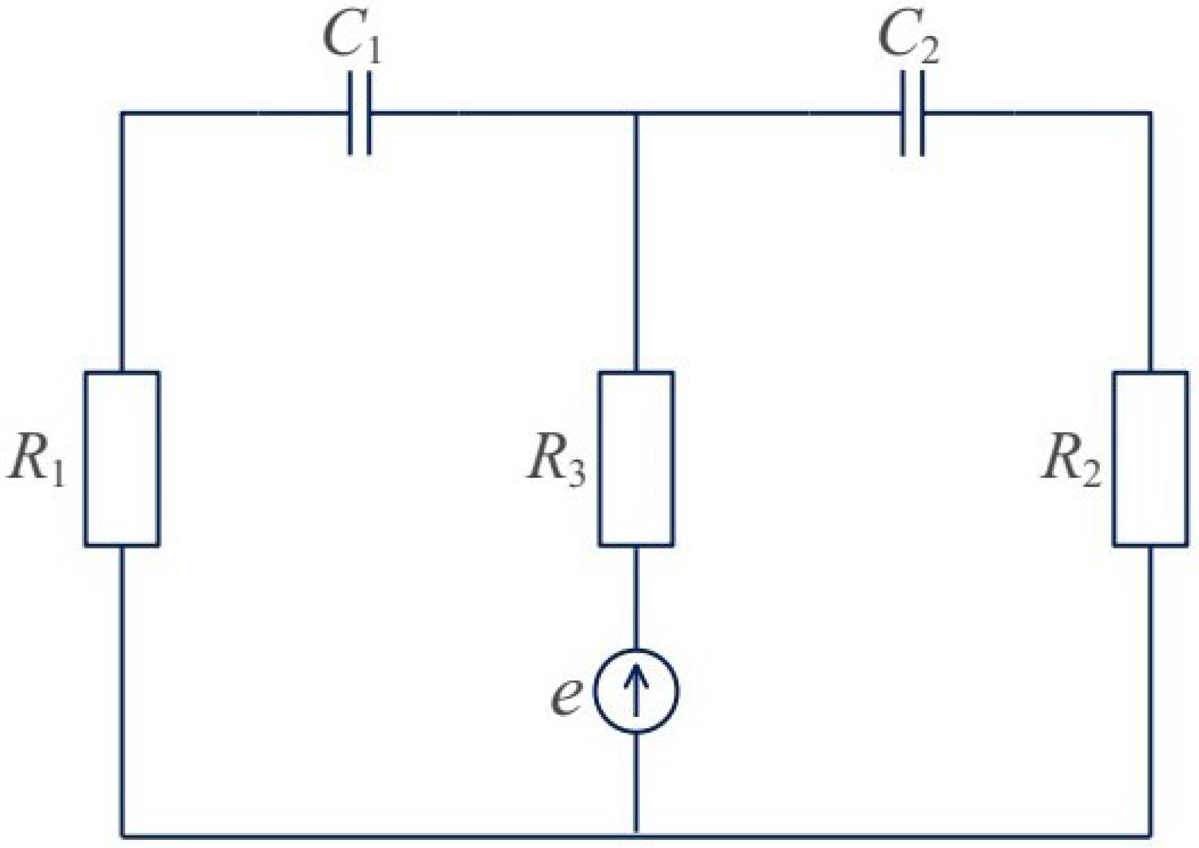
6.1. RC Circuit Systems

The circuit shown in Figure 1 is a fractional RC circuit. It includes source e, resistances $R_1, R_2$ and $R_3$ and fractional element Capacitor $C_1$ and $C_2$; both of them are of $\alpha$. Denote $v(t)$ as voltage, let $x_1(t)=v_{C_1},x_2(t)=v_{C_2}$ and $u(t)=e$ is the source voltage; $u(t)$ and $y(t)$ are input and output vectors, respectively. Set its parameters as follows: $C_1=3\times {10}^4$ µF, $C_2=3\times {10}^4$ µF, $R_1=10\mathsf{\Omega },R_2=20\mathsf{\Omega },R_3=30\mathsf{\Omega }$. Using Kirchhoff’s law, we can write the following systems:

$$({{}_{0}D}^{\alpha ,\rho }{x}_1)(t)=-\frac{R_2+R_3}{C_{1}R}{x}_1(t)+\frac{R_3}{C_{1}R}{x}_2(t)+\frac{R_2}{C_{1}R}u(t)$$

(49)

$$({{}_{0}D}^{\alpha ,\rho }{x}_2)(t)=\frac{R_3}{C_{2}R}{x}_1(t)-\frac{R_1+R_3}{C_{2}R}{x}_2(t)+\frac{R_1}{C_{2}R}u(t)$$

(50)

where $R=[R_1(R_2+R_3)+R_2{R}_3]$ and choose

$$y(t)=x_1(t)+x_2(t)$$

(51)

The Systems Equations (49)–(51) can be rewritten into the following system

$$({{}_{0}D}^{\alpha ,\rho }x)(t)=Ax(t)+Bu(t)$$

(52)

$$y(t)=Cx(t)$$

(53)

where

$$A=\left[\begin{array}{cc}-\frac{R_2+R_3}{C_{1}R}& \frac{R_3}{C_{1}R}\\ \frac{R_3}{C_{2}R}& -\frac{R_1+R_3}{C_{2}R}\end{array}\right],B=\left[\begin{array}{c}\frac{R_2}{C_{1}R}\\ \frac{R_1}{C_{2}R}\end{array}\right],C=\left[\begin{array}{cc}1& 1\end{array}\right].$$

(54)

From (54), we have

$$A=\left[\begin{array}{cc}-1.515& 0.909\\ 0.682& -0.909\end{array}\right],B=\left[\begin{array}{c}0.606\\ 0.227\end{array}\right],C=\left[\begin{array}{cc}1& 1\end{array}\right].$$

(55)

According to (36),

$$Q_r=\left[\begin{array}{cc}B& AB\end{array}\right]=\left[\begin{array}{cc}0.606& -0.71175\\ 0.227& 0.20695\end{array}\right],rank{Q}_r=2.$$

(56)

From Theorem 11 it follows that the fractional RC circuit is reachable.

Also, from Theorem 13 it follows that

$$Q_o=\left[\begin{array}{c}C\\ CA\end{array}\right]=\left[\begin{array}{cc}1& 1\\ \frac{R_3}{C_{2}R}-\frac{R_2+R_3}{C_{1}R}& \frac{R_3}{C_{1}R}-\frac{R_1+R_3}{C_{2}R}\end{array}\right]=\left[\begin{array}{cc}1& 1\\ -0.833& 0\end{array}\right],rank{Q}_o=2$$

(57)

the fractional RC circuit is observable.

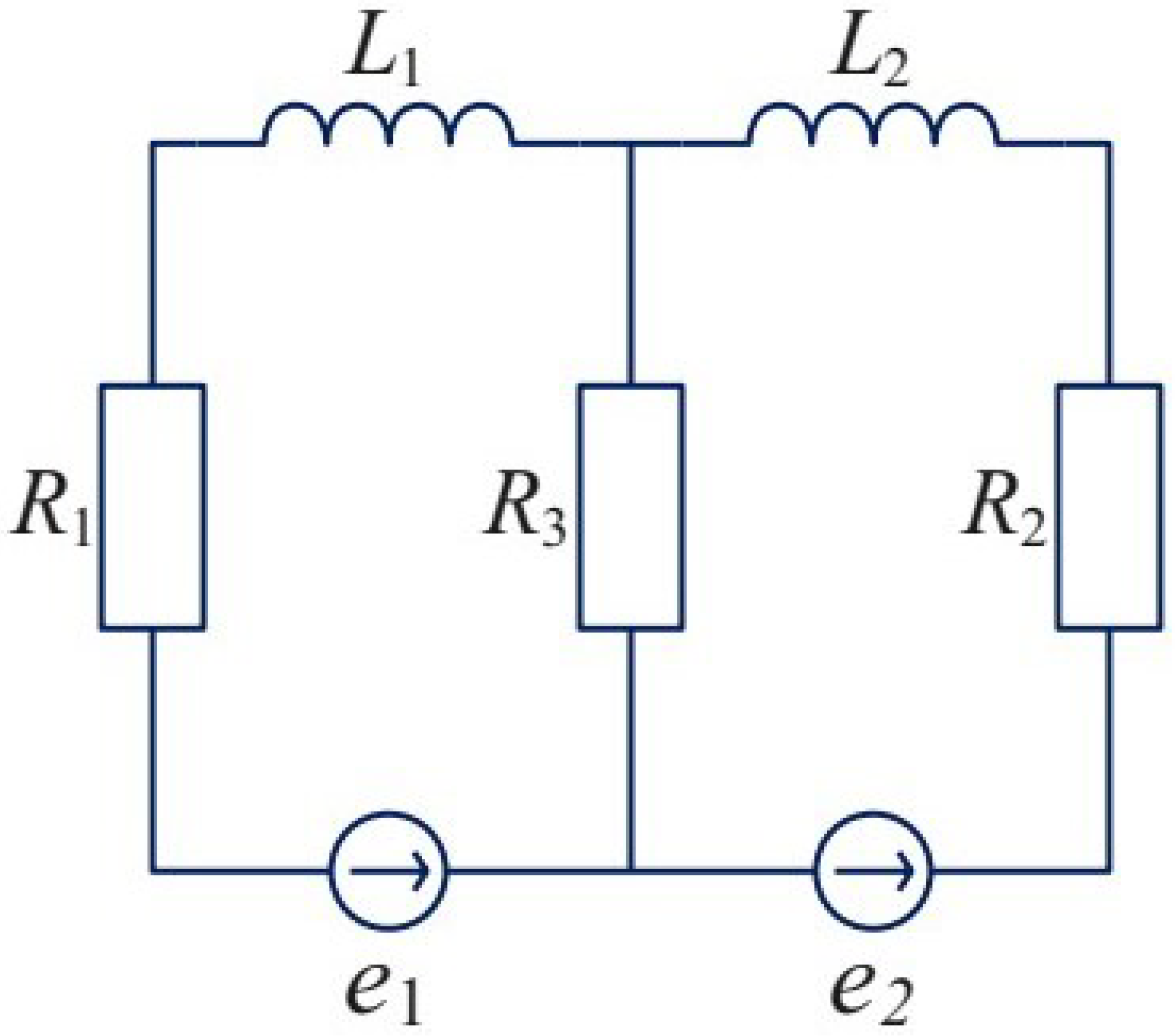
6.2. RL Circuit Systems

The circuit shown in Figure 2 is a fractional RL circuit. It includes sources $e_1,e_2$, resistances $R_1, R_2$ and $R_3$, and fractional element Capacitor $L_1$ and $L_2$, both of them are of $\alpha$. Denote $i(t)$ as current, let $x_1(t)=i_{L_1},x_2(t)=i_{L_2}$ and $u(t)$ is the source voltage; $u(t)$ and $y(t)$ are input and output vectors, respectively. Set its parameters as follows: $L_1=0.6H,L_2=0.8H,R_1=300\mathsf{\Omega },R_2=400\mathsf{\Omega },R_3=500\mathsf{\Omega }$.

Using Kirchhoff’s law, we can obtain the following systems equations:

$$({{}_{0}D}^{\alpha ,\rho }{x}_1)(t)=-\frac{R_1+R_3}{L_1}{x}_1(t)+\frac{R_3}{L_1}{x}_2(t)+\frac{1}{L_1}{e}_1$$

(58)

$$({{}_{0}D}^{\alpha ,\rho }{x}_2)(t)=\frac{R_3}{L_2}{x}_1(t)-\frac{R_2+R_3}{L_2}{x}_2(t)+\frac{1}{L_2}{e}_2$$

(59)

and choose

$$y(t)=R_1{x}_1(t)+R_2{x}_2(t)$$

(60)

The system Equations (58)–(60) can be rewritten into the following systems equations:

$$({{}_{0}D}^{\alpha ,\rho }x)(t)=Ax(t)+Bu(t)$$

(61)

$$y(t)=Cx(t)$$

(62)

where

$$A=\left[\begin{array}{cc}-\frac{R_1+R_3}{L_1}& \frac{R_3}{L_1}\\ \frac{R_3}{L_2}& -\frac{R_2+R_3}{L_2}\end{array}\right],B=\left[\begin{array}{cc}\frac{1}{L_1}& 0\\ 0& \frac{1}{L_2}\end{array}\right],C=\left[\begin{array}{cc}{R}_1& R_2\end{array}\right],u(t)=\left[\begin{array}{c}{e}_1\\ e_2\end{array}\right].$$

(63)

From (63), we have

$$A=\left[\begin{array}{cc}-1.3& 0.8\\ 0.6& -1.1\end{array}\right],B=\left[\begin{array}{cc}1.7& 0\\ 0& 1.25\end{array}\right],C=\left[\begin{array}{cc}300& 400\end{array}\right].$$

(64)

According to (36),

$$Q_r=\left[\begin{array}{cc}B& AB\end{array}\right]=\left[\begin{array}{cccc}1.7& 0& -2.2& 1\\ 0& 1.25& 1& 1.4\end{array}\right],rank{Q}_r=2.$$

(65)

From Theorem 11 it follows that the fractional RL circuit is reachable.

Also, from Theorem 13 it follows that

$$Q_o=\left[\begin{array}{c}C\\ CA\end{array}\right]=\left[\begin{array}{cc}300& 400\\ -150& -200\end{array}\right],rank{Q}_o=2$$

(66)

the fractional RL circuit is observable.

6.3. RC, RL Circuit Systems with Different Parameters $\rho$

Consider the RC electrical circuit (49–51) described by the left generalized fractional derivative with $C_1=3\times {10}^4$ µF, $C_2=3\times {10}^4$ µF, $R_1=10\mathsf{\Omega },R_2=20\mathsf{\Omega },R_3=30\mathsf{\Omega }$ and $e=6$. The numerical simulations for the circuit with $\alpha =0.85$ and $\rho =0.8$ are depicted in Figure 3. In the RC circuit described by (49–51) with $\alpha =0.85$, the relationship between the states and different parameters $\rho$ is shown in Figure 4.

Consider the RL electrical circuit (58–60) described by the left generalized fractional derivative with $L_1=0.6H,L_2=0.8H,R_1=300\mathsf{\Omega },R_2=400\mathsf{\Omega },R_3=500\mathsf{\Omega },e_1=23.56$ and $e_2=5.89$. The numerical simulations for the circuit with $\alpha =0.85$ and $\rho =0.8$ are depicted in Figure 5. And the relationship between states and different parameters in RL circuit described by (58–60) with $\alpha =0.85$ are depicted in Figure 6.

7. Conclusions

In this work, we use the differential equations based on the generalized fractional derivative to describe linear electrical circuits systems, and discuss the positivity of the electrical circuits systems, methods of checking the positivity of the systems are also presented. The main work is to deduce the checking method of reachability and observability of fractional order positive linear electrical circuit systems described by generalized fractional derivative. The $\rho$-Laplace transform of a Mittage-Leffler function with matrix form is proved, and the conditions of this transformation are also given. At the end of the paper, illustrative examples of RLC, RC and RL electrical circuits systems are presented, the influence of parameter $\rho$ on the state trajectory is observed, and it is found that parameter $\rho$ has an influence on the slope of the state trajectory. The state trajectory of the circuit system described by the generalized fractional derivative is more realistic.

References

1. Sene, N.; Fall, A. Homotopy perturbation ρ-Laplace transform method and its application to the fractional diffusion equation and the fractional diffusion-reaction equation. Fractal Fract. 2019, 3, 14. [Google Scholar] [CrossRef] [Green Version]
2. Dos Santos, M.; Gomez, I. A fractional Fokker-Planck equation for non-singular kernel operators. J. Stat. Mech. Theory Exp. 2018, 2018, 123205. [Google Scholar] [CrossRef] [Green Version]
3. Dos Santos, M. Fractional Prabhakar derivative in diffusion equation with non-static stochastic resetting. Physics 2019, 1, 40–58. [Google Scholar] [CrossRef] [Green Version]
4. Sene, N.; Abdelmalek, K. Analysis of the fractional diffusion equations described by Atangana-Baleanu-Caputo fractional derivative. Chaos Soli. Fract. 2019, 127, 158–164. [Google Scholar] [CrossRef]
5. Atangana, A.; Baleanu, D. New fractional derivatives with nonlocal and non-singular kernel: Theory and application to heat transfer model. Therm. Sci. 2016, 20, 763–769. [Google Scholar] [CrossRef] [Green Version]
6. Katugampola, U. A new approach to generalized fractional derivatives. Bul. Math. Anal.Appl. 2014, 6, 1–15. [Google Scholar]
7. Fahd, J.; Abdeljawad, T. A modified Laplace transform for certain generalized fractional operators. Results Nonlinear Anal. 2018, 1, 88–98. [Google Scholar]
8. Hristov, J. On the Atangana-Baleanu derivative and its relation to the fading memory concept: The diffusion equation formulation. In Trends in Theory and Applications of Fractional Derivatives with Mittag-Leffler Kernel; Gomez, J., Torres, L., Escobar, R., Eds.; Springer: Cham, Switzerland, 2019; pp. 175–193. [Google Scholar]
9. Abdeljawad, T. On conformable fractional calculus. J. Comput. Appl. Math. 2013, 279, 57–66. [Google Scholar] [CrossRef]
10. Khan, H.; Jarad, F.; Abdeljawad, T.; Khan, A. A singular ABC-fractional differential equation with ρ-Laplacian operator. Chaos Solitons Fractals 2019, 129, 56–61. [Google Scholar] [CrossRef]
11. Sene, N. Fractional input stability for electrical circuits described by the Riemann-Liouville and the Caputo fractional derivatives. AIMS Math. 2019, 4, 147–165. [Google Scholar] [CrossRef]
12. Kaczorek, T. Selected Problems of Fractional Systems Theory; Springer: Berlin/Heidelberg, Germany, 2011. [Google Scholar]
13. Kilbas, A.; Srivastava, H.; Trujillo, J. Theory and Application of Fractional Differential Equations, Volume 13; North-Holland Mathematics Studies; Elsevier Science: Amsterdam, The Netherlands, 2006; Volume 204, 523p. [Google Scholar]
14. Kaczorek, T.; Rogowski, K. Fractional Linear Systems and Electrical Circuits; Springer: Cham, Switzerland, 2015. [Google Scholar]
15. Aguilar, J. Behavior characteristics of a cap-resistor, memcapacitor, and a memristor from the response obtained of RC and RL electrical circuits described by fractional differential equations. Turk. J. Electr. Eng. Comput. Sci. 2016, 24, 1421–1433. [Google Scholar] [CrossRef] [Green Version]
16. Gomez-Aguilar, J.; Atangana, A. New insight in fractional differentiation: Power, exponential decay and Mittag-Leffler laws and applications. Eur. Phys. J. Plus 2017, 132, 13. [Google Scholar] [CrossRef]
17. Aguilar, J.; Baleanu, D. Baleanu, Fractional Transmission Line with Losses. Z. Naturforschung A 2014, 69, 539–546. [Google Scholar] [CrossRef] [Green Version]
18. Gomez-Aguilar, J.; Escobar-Jimenez, R.; OlivaresPeregrino, V.; Taneco-Hernandez, M.; Guerrero-Ramirez, G. Electrical circuits RC and RL involving fractional operators with bi-order. Adv. Mech. Eng. 2017, 9, 1–10. [Google Scholar] [CrossRef]
19. Morales-Delgado, V.; Gomez-Aguilar, J.; TanecoHernandez, M.; Escobar-Jimenez, R. Fractional operator without singular kernel: Applications to linear electrical circuits. Int. J. Circuit Theory Appl. 2018, 46, 2394–2419. [Google Scholar] [CrossRef]
20. Morales-Delgado, V.; Gomez-Aguilar, J.; TanecoHernandez, M. Analytical solutions of electrical circuits described by fractional conformable derivatives in Liouville-Caputo sense. AEU-Int. J. Electron. Commun. 2018, 85, 108–117. [Google Scholar] [CrossRef]
21. Gomez-Aguilar, J.; Morales-Delgado, V. Electrical circuits RC, LC, and RL described by AtanganaBaleanu fractional derivatives. Int. J. Circuit Theory Appl. 2017, 45, 1514–1533. [Google Scholar] [CrossRef]
22. Radwan, A.; Salama, K. Fractional-order RC and RL circuits. Circuits Syst. Signal Process. 2012, 31, 1901–1915. [Google Scholar] [CrossRef]
23. Sene, N.; Gomez-Aguilar, J. Analytical solutions of electrical circuits considering certain generalized fractional derivatives. Eur. Phys. J. Plus 2019, 134, 260. [Google Scholar] [CrossRef]
24. Si, X.; Yang, H. A new method for judgment and computation of stability and stabilization of fractional order positive systems with constraints. J. Shandong Univ. Sci. Technol. (Nat. Sci.) 2021, 40, 12–20. [Google Scholar]
25. Si, X.; Yang, H. Optimization approach to the constrained regulation problem for linear continuous-time fractional-order systems. Int. J. Nonlinear Sci. Numer. Simul. 2021, 22, 1–16. [Google Scholar] [CrossRef]
26. Ji, S.; Li, G. Existence of solution to nonlocal fractional differential inclusions via resolvent operators. J. Shandong Univ. Sci. Technol. (Nat. Sci.) 2021, 40, 103–108. [Google Scholar]
27. Kaczorek, T. Stability of positive continuous-time linear systems with delays. Bull. Pol. Acad. Sci. Tech. Sci. 2009, 57, 395–398. [Google Scholar]
28. Kaczorek, T. Stability Tests of Positive Fractional Continuous-time Linear Systems with Delays. TransNav Int. J. Mar. Navig. Saf. Sea Transp. 2013, 7, 211–215. [Google Scholar] [CrossRef]
29. Sene, N. Stability analysis of the generalized fractional differential equations with and without exogenous inputs. J. Nonlinear Sci. Appl. 2019, 12, 562–572. [Google Scholar] [CrossRef]
30. Yu, Z.; Sun, Y.; Dai, X. Stability and Stabilization of the Fractional-order Power System with Time Delay. IEEE Trans. Circuits Syst. 2021, 68, 3446–3450. [Google Scholar] [CrossRef]
31. Chao, C.; Chen, D.; Chiou, J. Stability Analysis and Robust Stabilization of Uncertain Fuzzy Time-Delay Systems. Mathematics 2021, 9, 2441. [Google Scholar] [CrossRef]
32. Sene, N. Stability analysis of electrical RLC circuit described by the Caputo-Liouville generalized fractional derivative. Alex. Eng. J. 2020, 59, 2083–2090. [Google Scholar] [CrossRef]
33. Erdelyi, A.; Kober, H. Some remarks on hankel transforms. Q. J. Math. 1940, 11, 212–221. [Google Scholar] [CrossRef]
34. Herrmann, R. Towards a geometric interpretation of generalized fractional integrals—Erdelyi-Kober type integrals on RN as an example. Fract. Calc. Appl. Anal. 2014, 17, 361–370. [Google Scholar] [CrossRef] [Green Version]
35. Jerzy, K. Controllability of Fractional Linear Systems with Delays. In Proceedings of the 25th International Conference on Methods and Models in Automation and Robotics (MMAR), Międzyzdroje, Poland, 23–26 August 2021; Institute of Electrical and Electronics Engineers: New York, NY, USA, 2021. [Google Scholar]
36. Gu, P.; Chen, Y.; Tian, S. Learnability of Linear Fractional-Order ILC Systems. IEEE Trans. Circuits Syst. 2021, 68, 963–967. [Google Scholar] [CrossRef]
37. Kaczorek, T. Reachability and controllability to zero of positive fractional discrete-time systems. In Proceedings of the European Control Conference (ECC), Kos, Greece, 2–5 July 2007; Institute of Electrical and Electronics Engineers: New York, NY, USA, 2007. [Google Scholar]
38. Kaczorek, T. Invariant properties of positive linear electrical circuit. Arch. Elektrotech. 2019, 68, 875–890. [Google Scholar]
39. Yuan, T.; Yang, H. Invariance of reachability and observability for fractional positive linear electrical circuit with delays. Arch. Elektrotech. 2021, 70, 513–530. [Google Scholar]
Figure 1. The fractional RC circuit.
Mathematics 09 02856 g001
Figure 2. The fractional RL circuit.
Mathematics 09 02856 g002
Figure 3. Voltage trajectories across the capacitors described by the fractional RC circuit (49–51).
Mathematics 09 02856 g003
Figure 4. States with different parameters in RC circuit (49–51): (a) Trajectory of x 1 with different parameters; (b) Trajectory of x 2 with different parameters.
Mathematics 09 02856 g004
Figure 5. Current trajectories across the inductors described by the fractional RL circuit (58–60).
Mathematics 09 02856 g005
Figure 6. Relationship between states and different parameters in RL circuit (58–60): (a) Trajectory of x 1 with different parameters; (b) Trajectory of x 2 with different parameters.
Mathematics 09 02856 g006
Publisher’s Note: MDPI stays neutral with regard to jurisdictional claims in published maps and institutional affiliations.