
Faster and Slower Soliton Phase Shift: Oceanic Waves Affected by Earth Rotation


Abstract
:1. Introduction
- (a)
- ;
- (b)
- ;
- (c)
- ;
- (d)
- , provided
- (e)
- , where is a constant.
2. Analytical Solutions
3. Solutions’ Accuracy
4. Results and Discussion
5. Conclusions
Author Contributions
Funding
Institutional Review Board Statement
Informed Consent Statement
Data Availability Statement
Acknowledgments
Conflicts of Interest
References
- Baskonus, H.M.; Osman, M.; Ramzan, M.; Tahir, M.; Ashraf, S. On pulse propagation of soliton wave solutions related to the perturbed Chen–Lee–Liu equation in an optical fiber. Opt. Quantum Electron. 2021, 53, 1–17. [Google Scholar]
- Sarwar, S. New soliton wave structures of nonlinear (4 + 1)-dimensional Fokas dynamical model by using different methods. Alex. Eng. J. 2021, 60, 795–803. [Google Scholar] [CrossRef]
- Kumar, S.; Almusawa, H.; Hamid, I.; Akbar, M.A.; Abdou, M. Abundant analytical soliton solutions and Evolutionary behaviors of various wave profiles to the Chaffee–Infante equation with gas diffusion in a homogeneous medium. Results Phys. 2021, 30, 104866. [Google Scholar] [CrossRef]
- Zhao, J.; Manafian, J.; Zaya, N.E.; Mohammed, S.A. Multiple rogue wave, lump-periodic, lump-soliton, and interaction between k-lump and k-stripe soliton solutions for the generalized KP equation. Math. Methods Appl. Sci. 2021, 44, 5079–5098. [Google Scholar] [CrossRef]
- Ismael, H.F.; Ma, W.X.; Bulut, H. Dynamics of soliton and mixed lump-soliton waves to a generalized Bogoyavlensky-Konopelchenko equation. Phys. Scr. 2021, 96, 035225. [Google Scholar] [CrossRef]
- Nisar, K.S.; Ilhan, O.A.; Abdulazeez, S.T.; Manafian, J.; Mohammed, S.A.; Osman, M. Novel multiple soliton solutions for some nonlinear PDEs via multiple Exp-function method. Results Phys. 2021, 21, 103769. [Google Scholar] [CrossRef]
- Kumar, S.; Niwas, M.; Osman, M.; Abdou, M. Abundant different types of exact soliton solution to the (4 + 1)-dimensional Fokas and (2 + 1)-dimensional breaking soliton equations. Commun. Theor. Phys. 2021, 73, 105007. [Google Scholar] [CrossRef]
- Raza, N.; Rafiq, M.H.; Kaplan, M.; Kumar, S.; Chu, Y.M. The unified method for abundant soliton solutions of local time fractional nonlinear evolution equations. Results Phys. 2021, 22, 103979. [Google Scholar] [CrossRef]
- Osman, M.; Almusawa, H.; Tariq, K.U.; Anwar, S.; Kumar, S.; Younis, M.; Ma, W.X. On global behavior for complex soliton solutions of the perturbed nonlinear Schrödinger equation in nonlinear optical fibers. J. Ocean. Eng. Sci. 2021, in press. [Google Scholar] [CrossRef]
- Rizvi, S.; Seadawy, A.; Ashraf, M.; Bashir, A.; Younis, M.; Baleanu, D. Multi-wave, homoclinic breather, M-shaped rational and other solitary wave solutions for coupled-Higgs equation. Eur. Phys. J. Spec. Top. 2021, 230, 3519–3532. [Google Scholar] [CrossRef]
- Ismael, H.F.; Bulut, H. Multi soliton solutions, M-lump waves and mixed soliton-lump solutions to the awada-Kotera equation in (2 + 1)-dimensions. Chin. J. Phys. 2021, 71, 54–61. [Google Scholar] [CrossRef]
- Feng, Y.; Wang, X.; Bilige, S. Evolutionary behavior and novel collision of various wave solutions to (3 + 1)-dimensional generalized Camassa–Holm Kadomtsev–Petviashvili equation. Nonlinear Dyn. 2021, 104, 4265–4275. [Google Scholar] [CrossRef]
- Kumar, S.; Jiwari, R.; Mittal, R.; Awrejcewicz, J. Dark and bright soliton solutions and computational modeling of nonlinear regularized long wave model. Nonlinear Dyn. 2021, 104, 661–682. [Google Scholar] [CrossRef]
- Liu, C. The Gaussian soliton in the Fermi–Pasta–Ulam chain. Nonlinear Dyn. 2021, 106, 899–905. [Google Scholar] [CrossRef]
- Ma, W.X.; Osman, M.; Arshed, S.; Raza, N.; Srivastava, H. Practical analytical approaches for finding novel optical solitons in the single-mode fibers. Chin. J. Phys. 2021, 72, 475–486. [Google Scholar] [CrossRef]
- Kuo, C.K.; Chen, Y.C.; Wu, C.W.; Chao, W.N. Novel solitary and resonant multi-soliton solutions to the (3 + 1)-dimensional potential-YTSF equation. Mod. Phys. Lett. B 2021, 35, 2150326. [Google Scholar] [CrossRef]
- Zahran, E.H.; Khater, M.M. Modified extended tanh-function method and its applications to the Bogoyavlenskii equation. Appl. Math. Model. 2016, 40, 1769–1775. [Google Scholar] [CrossRef]
- Abdelrahman, M.A.; Zahran, E.H.; Khater, M.M. The Exp −ϕ(ξ)-expansion method and its application for solving nonlinear evolution equations. Int. J. Mod. Nonlinear Theory Appl. 2015, 4, 37. [Google Scholar] [CrossRef] [Green Version]
- Khater, M.M.; Seadawy, A.R.; Lu, D. Dispersive solitary wave solutions of new coupled Konno-Oono, Higgs field and Maccari equations and their applications. J. King Saud Univ.-Sci. 2018, 30, 417–423. [Google Scholar] [CrossRef]
- Khater, M.M. Extended exp Expansion method for Solving the Generalized Hirota-Satsuma Coupled KdV System. Glob. J. Sci. Front. Res. F Math. Decis. Sci. 2015, 15, 1–15. [Google Scholar]
- Wang, K.L.; Yao, S.W. Numerical method for fractional Zakharov-Kuznetsov equations with He’s fractional derivative. Therm. Sci. 2019, 23, 2163–2170. [Google Scholar] [CrossRef]
- Wang, K.L.; Liu, S.Y. He’s fractional derivative for non-linear fractional heat transfer equation. Therm. Sci. 2016, 20, 793–796. [Google Scholar] [CrossRef]
- Zuo, Y.; Liu, H. A fractal rheological model for sic paste using a fractal derivative. J. Appl. Comput. Mech. 2020, 7, 13–18. [Google Scholar]
- Ma, W.X.; Osman, M.; Arshed, S.; Raza, N.; Srivastava, H. Different analytical approaches for finding novel optical solitons in the single-mode fibers. Chin. J. Phys. 2021, 27, 475–486. [Google Scholar] [CrossRef]
- Khan, Y. A novel type of soliton solutions for the Fokas–Lenells equation arising in the application of optical fibers. Mod. Phys. Lett. B 2021, 35, 2150058. [Google Scholar] [CrossRef]
- Kuo, C.K.; Ghanbari, B. On novel resonant multi-soliton and wave solutions to the (3 + 1)-dimensional GSWE equation via three effective approaches. Results Phys. 2021, 26, 104421. [Google Scholar] [CrossRef]
- Alsaedi, A.; Ahmad, B.; Kirane, M.; Torebek, B.T. Blowing-up solutions of the time-fractional dispersive equations. Adv. Nonlinear Anal. 2021, 10, 952–971. [Google Scholar] [CrossRef]
- Wang, K.J. On new abundant exact traveling wave solutions to the local fractional Gardner equation defined on Cantor sets. Math. Methods Appl. Sci. 2021, 1, 12. [Google Scholar] [CrossRef]
- Fang, Y.; Wu, G.Z.; Wang, Y.Y.; Dai, C.Q. Data-driven femtosecond optical soliton excitations and parameters discovery of the high-order NLSE using the PINN. Nonlinear Dyn. 2021, 105, 603–616. [Google Scholar] [CrossRef]
- Alfalqi, S.H.; Alzaidi, J.F.; Zhang, Y.F.; Salama, S.A.; Khater, M.M. Plenty accurate soliton wave solutions of the prototype of an excitable system. AIP Adv. 2021, 11, 095315. [Google Scholar] [CrossRef]
- Han, C.; Wang, Y.L.; Li, Z.Y. Numerical solutions of space fractional variable-coefficient KdV-modified KdV equation by Fourier spectral method. Fractals 2021, 0, 2150246. [Google Scholar] [CrossRef]
- Manafian, J.; Lakestani, M.; Bekir, A. Comparison between the generalized tanh–coth and the (G′/G)-expansion methods for solving NPDEs and NODEs. Pramana 2016, 87, 1–14. [Google Scholar] [CrossRef]
- Heris, J.M.; Lakestani, M. Solitary wave and periodic wave solutions for variants of the KdV-Burger and the K (n, n)-Burger equations by the generalized tanh-coth method. Commun. Numer. Anal. 2013, 2013, 1–18. [Google Scholar] [CrossRef] [Green Version]
- Dai, D.D.; Ban, T.T.; Wang, Y.L.; Zhang, W. The piecewise reproducing kernel method for the time variable fractional order advection-reaction-diffusion equations. Therm. Sci. 2021, 25, 21. [Google Scholar] [CrossRef]
- Khater, M.M.; Lu, D. Analytical versus numerical solutions of the nonlinear fractional time–space telegraph equation. Mod. Phys. Lett. B 2021, 35, 2150324. [Google Scholar] [CrossRef]
- Khater, M.M. Diverse solitary and Jacobian solutions in a continually laminated fluid with respect to shear flows through the Ostrovsky equation. Mod. Phys. Lett. B 2021, 35, 2150220. [Google Scholar] [CrossRef]
- Köroğlu, C.; Öziş, T. A novel traveling wave solution for Ostrovsky equation using Exp-function method. Comput. Math. Appl. 2009, 58, 2142–2146. [Google Scholar] [CrossRef] [Green Version]
- Yusufoğlu, E.; Bekir, A. A travelling wave solution to the Ostrovsky equation. Appl. Math. Comput. 2007, 186, 256–260. [Google Scholar] [CrossRef]
- Khalil, R.; Al Horani, M.; Yousef, A.; Sababheh, M. A new definition of fractional derivative. J. Comput. Appl. Math. 2014, 264, 65–70. [Google Scholar] [CrossRef]
- Abdeljawad, T. On conformable fractional calculus. J. Comput. Appl. Math. 2015, 279, 57–66. [Google Scholar] [CrossRef]
- Atangana, A.; Baleanu, D.; Alsaedi, A. New properties of conformable derivative. Open Math. 2015, 3, 000010151520150081. [Google Scholar] [CrossRef]
- Li, Z.B.; He, J.H. Fractional complex transform for fractional differential equations. Math. Comput. Appl. 2010, 15, 970–973. [Google Scholar] [CrossRef] [Green Version]
- Li, Z.B. An extended fractional complex transform. Int. J. Nonlinear Sci. Numer. Simul. 2010, 11, 335–338. [Google Scholar] [CrossRef]
- Khater, M.M.; Salama, S.A. Novel analytical simulations of the complex nonlinear Davey–Stewartson equations in the gravity–capillarity surface wave packets. J. Ocean. Eng. Sci. 2021, in press. [Google Scholar] [CrossRef]


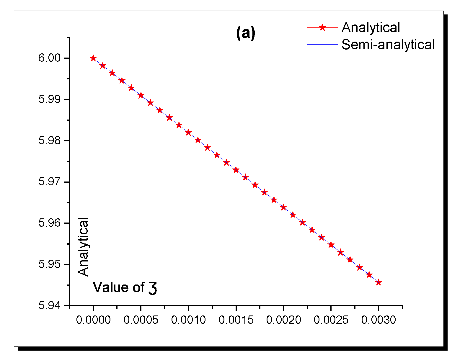
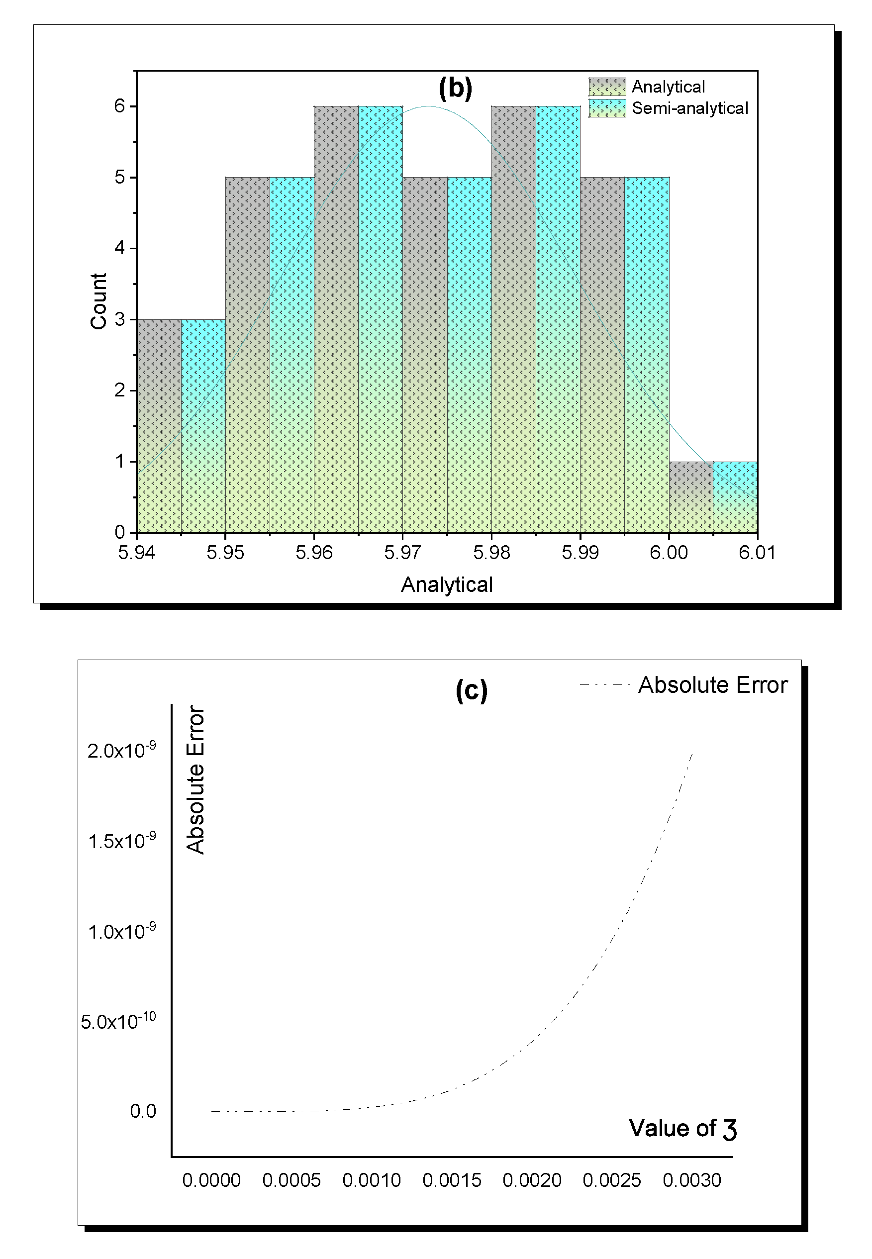
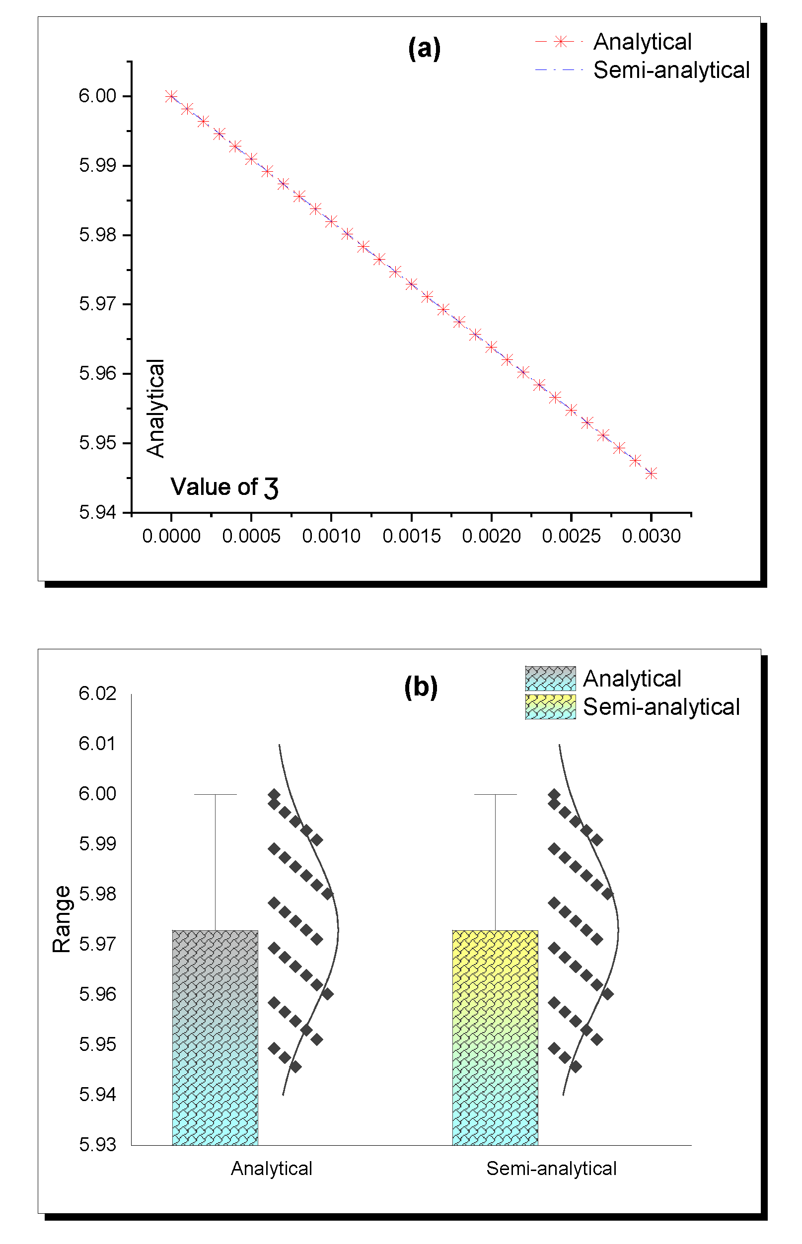
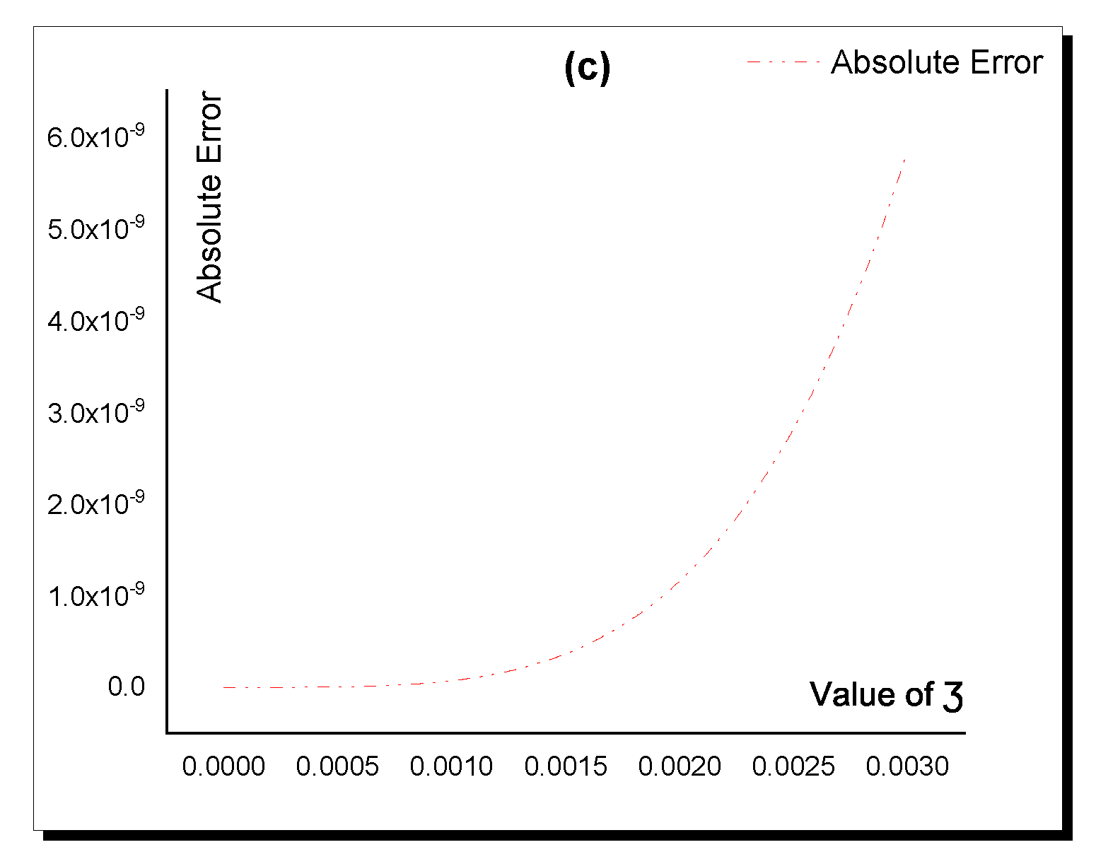
| Value of | Analytical | Semi-Analytical | Absolute Error |
|---|---|---|---|
| 0 | 6 | 6 | 0 |
| 0.0001 | 5.99819964 | 5.99819964 | 2.66454 |
| 0.0002 | 5.99639856 | 5.99639856 | 3.81917 |
| 0.0003 | 5.994596762 | 5.994596762 | 1.97176 |
| 0.0004 | 5.992794244 | 5.992794244 | 6.12843 |
| 0.0005 | 5.990991008 | 5.990991008 | 1.50635 |
| 0.0006 | 5.989187053 | 5.989187053 | 3.12017 |
| 0.0007 | 5.987382381 | 5.987382381 | 5.78648 |
| 0.0008 | 5.985576991 | 5.985576991 | 9.87299 |
| 0.0009 | 5.983770884 | 5.983770884 | 1.58265 |
| 0.001 | 5.98196406 | 5.98196406 | 2.41354 |
| 0.0011 | 5.98015652 | 5.98015652 | 3.53566 |
| 0.0012 | 5.978348264 | 5.978348264 | 5.00977 |
| 0.0013 | 5.976539292 | 5.976539292 | 6.90425 |
| 0.0014 | 5.974729605 | 5.974729605 | 9.29203 |
| 0.0015 | 5.972919203 | 5.972919203 | 1.22514 |
| 0.0016 | 5.971108086 | 5.971108086 | 1.58691 |
| 0.0017 | 5.969296256 | 5.969296255 | 2.02347 |
| 0.0018 | 5.967483711 | 5.967483711 | 2.5447 |
| 0.0019 | 5.965670453 | 5.965670452 | 3.16081 |
| 0.002 | 5.963856482 | 5.963856481 | 3.88278 |
| 0.0021 | 5.962041798 | 5.962041797 | 4.72212 |
| 0.0022 | 5.960226401 | 5.960226401 | 5.69098 |
| 0.0023 | 5.958410293 | 5.958410292 | 6.80211 |
| 0.0024 | 5.956593473 | 5.956593472 | 8.06888 |
| 0.0025 | 5.954775941 | 5.95477594 | 9.50533 |
| 0.0026 | 5.952957699 | 5.952957698 | 1.11259 |
| 0.0027 | 5.951138746 | 5.951138745 | 1.29459 |
| 0.0028 | 5.949319083 | 5.949319081 | 1.49812 |
| 0.0029 | 5.94749871 | 5.947498708 | 1.72481 |
| 0.003 | 5.945677628 | 5.945677626 | 1.97638 |
| Value of | Analytical | Semi-Analytical | Absolute Error |
|---|---|---|---|
| 0 | 6 | 6 | 0 |
| 0.0001 | 5.99819964 | 5.99819964 | 7.10543 |
| 0.0002 | 5.99639856 | 5.99639856 | 1.15463 |
| 0.0003 | 5.994596762 | 5.994596762 | 5.86198 |
| 0.0004 | 5.992794244 | 5.992794244 | 1.84031 |
| 0.0005 | 5.990991008 | 5.990991008 | 4.50218 |
| 0.0006 | 5.989187053 | 5.989187053 | 9.33031 |
| 0.0007 | 5.987382381 | 5.987382381 | 1.72893 |
| 0.0008 | 5.985576991 | 5.985576991 | 2.94902 |
| 0.0009 | 5.983770884 | 5.983770884 | 4.72404 |
| 0.001 | 5.98196406 | 5.98196406 | 7.20011 |
| 0.0011 | 5.98015652 | 5.98015652 | 1.05417 |
| 0.0012 | 5.978348264 | 5.978348264 | 1.49297 |
| 0.0013 | 5.976539292 | 5.976539292 | 2.05637 |
| 0.0014 | 5.974729605 | 5.974729605 | 2.76596 |
| 0.0015 | 5.972919203 | 5.972919203 | 3.64495 |
| 0.0016 | 5.971108086 | 5.971108086 | 4.71857 |
| 0.0017 | 5.969296256 | 5.969296256 | 6.01343 |
| 0.0018 | 5.967483711 | 5.967483711 | 7.55819 |
| 0.0019 | 5.965670453 | 5.965670453 | 9.38302 |
| 0.002 | 5.963856482 | 5.963856482 | 1.15199 |
| 0.0021 | 5.962041798 | 5.962041798 | 1.40024 |
| 0.0022 | 5.960226401 | 5.960226401 | 1.68662 |
| 0.0023 | 5.958410293 | 5.958410293 | 2.01482 |
| 0.0024 | 5.956593473 | 5.956593473 | 2.38874 |
| 0.0025 | 5.954775941 | 5.954775941 | 2.81244 |
| 0.0026 | 5.952957699 | 5.952957699 | 3.29015 |
| 0.0027 | 5.951138746 | 5.951138746 | 3.82628 |
| 0.0028 | 5.949319083 | 5.949319083 | 4.42541 |
| 0.0029 | 5.94749871 | 5.94749871 | 5.09228 |
| 0.003 | 5.945677628 | 5.945677628 | 5.83183 |
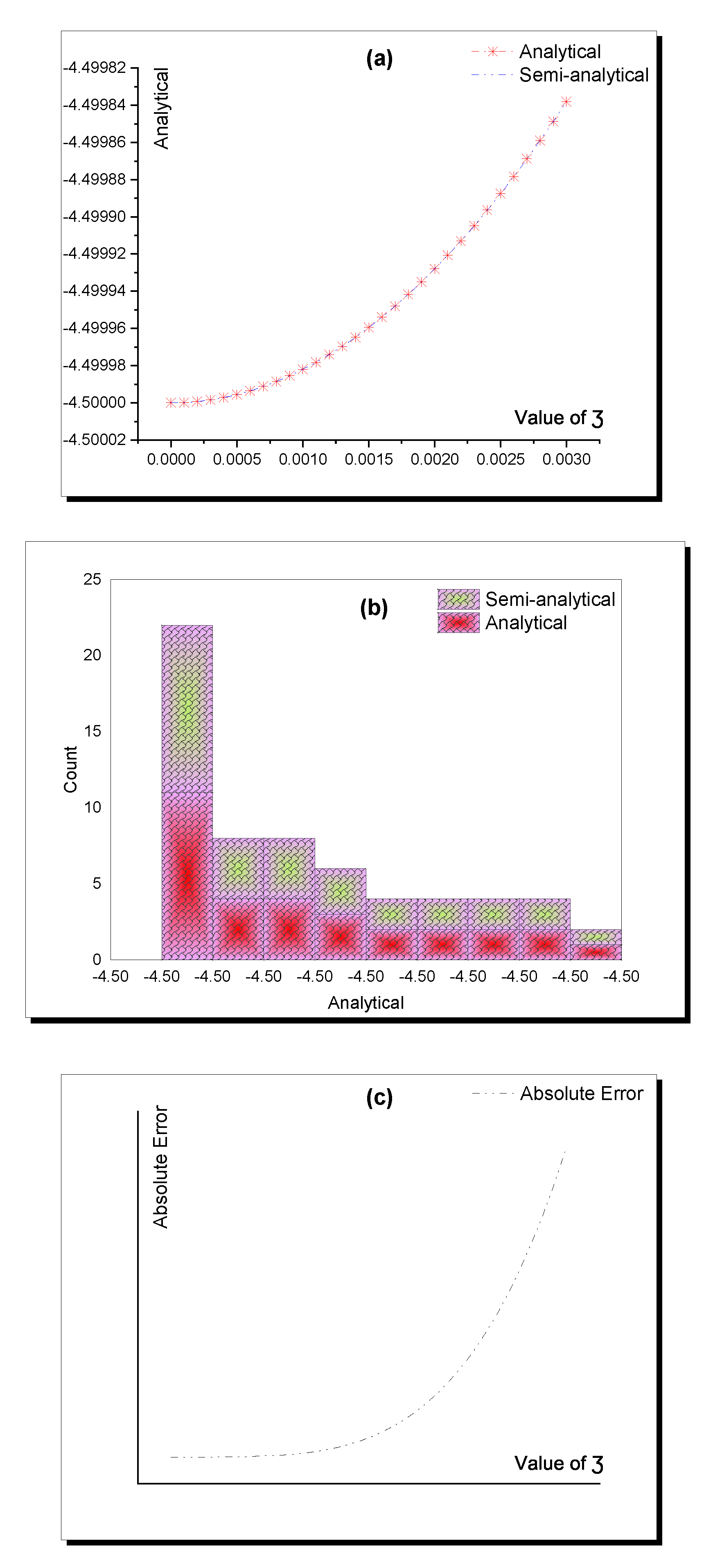
| Value of | Analytical | Semi-Analytical | Absolute Error |
|---|---|---|---|
| 0 | −4.5 | −4.5 | 0 |
| 0.0001 | −4.49999982 | −4.49999982 | 7.99361 |
| 0.0002 | −4.49999928 | −4.49999928 | 1.14575 |
| 0.0003 | −4.49999838 | −4.49999838 | 5.81757 |
| 0.0004 | −4.49999712 | −4.49999712 | 1.84475 |
| 0.0005 | −4.4999955 | −4.4999955 | 4.49862 |
| 0.0006 | −4.49999352 | −4.49999352 | 9.33209 |
| 0.0007 | −4.49999118 | −4.49999118 | 1.72866 |
| 0.0008 | −4.49998848 | −4.49998848 | 2.9492 |
| 0.0009 | −4.49998542 | −4.49998542 | 4.72387 |
| 0.001 | −4.499982 | −4.499982 | 7.19993 |
| 0.0011 | −4.49997822 | −4.49997822 | 1.05415 |
| 0.0012 | −4.49997408 | −4.49997408 | 1.49301 |
| 0.0013 | −4.49996958 | −4.49996958 | 2.0564 |
| 0.0014 | −4.49996472 | −4.49996472 | 2.76596 |
| 0.0015 | −4.4999595 | −4.499959501 | 3.64502 |
| 0.0016 | −4.49995392 | −4.499953921 | 4.71861 |
| 0.0017 | −4.49994798 | −4.499947981 | 6.01355 |
| 0.0018 | −4.499941681 | −4.499941681 | 7.55829 |
| 0.0019 | −4.499935021 | −4.499935022 | 9.38313 |
| 0.002 | −4.499928001 | −4.499928002 | 1.152 |
| 0.0021 | −4.499920621 | −4.499920622 | 1.40027 |
| 0.0022 | −4.499912881 | −4.499912883 | 1.68665 |
| 0.0023 | −4.499904781 | −4.499904783 | 2.01487 |
| 0.0024 | −4.499896322 | −4.499896324 | 2.3888 |
| 0.0025 | −4.499887502 | −4.499887505 | 2.81252 |
| 0.0026 | −4.499878322 | −4.499878325 | 3.29025 |
| 0.0027 | −4.499868783 | −4.499868786 | 3.82641 |
| 0.0028 | −4.499858883 | −4.499858887 | 4.42556 |
| 0.0029 | −4.499848623 | −4.499848628 | 5.09247 |
| 0.003 | −4.499838004 | −4.49983801 | 5.83205 |
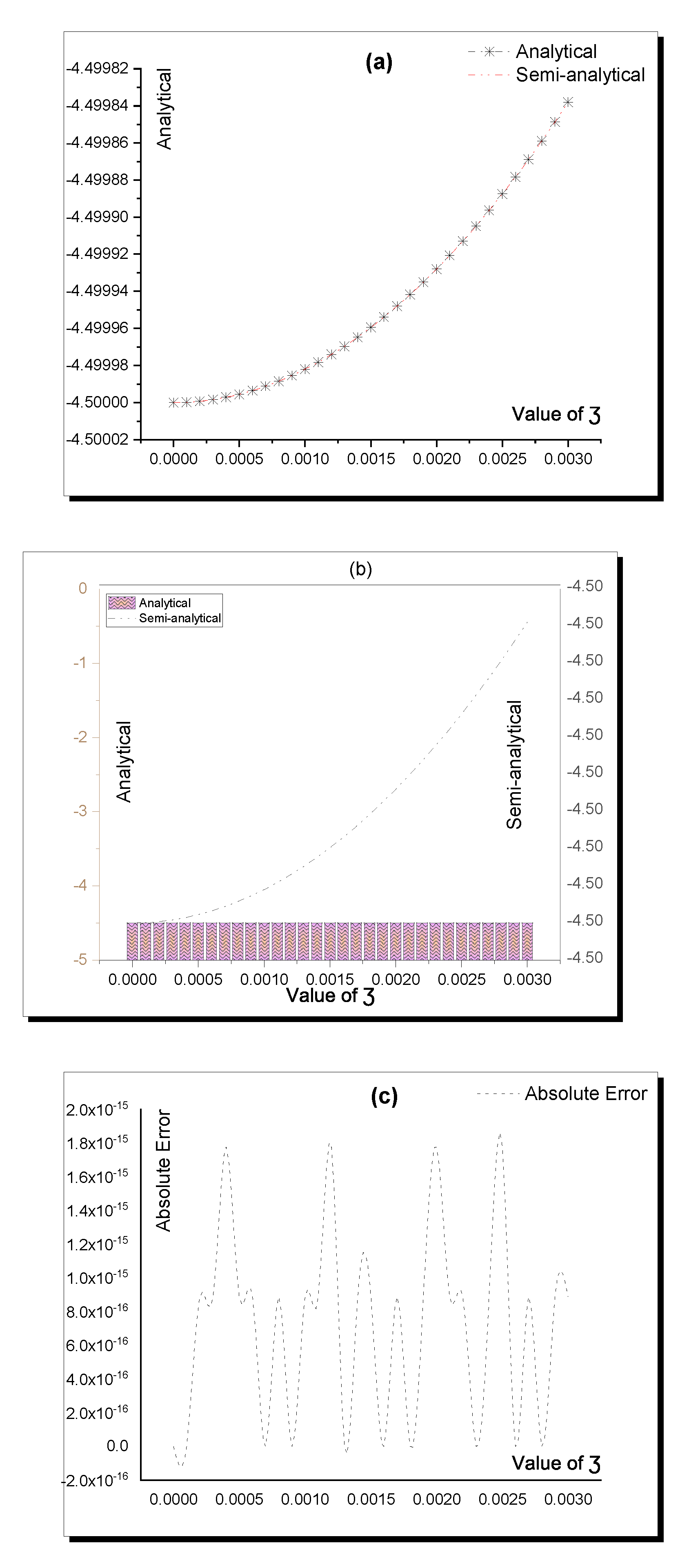
| Value of | Analytical | Semi-Analytical | Absolute Error |
|---|---|---|---|
| 0 | −4.5 | −4.5 | 0 |
| 0.0001 | −4.49999982 | −4.49999982 | 0 |
| 0.0002 | −4.49999928 | −4.49999928 | 8.88178 |
| 0.0003 | −4.49999838 | −4.49999838 | 8.88178 |
| 0.0004 | −4.49999712 | −4.49999712 | 1.77636 |
| 0.0005 | −4.4999955 | −4.4999955 | 8.88178 |
| 0.0006 | −4.49999352 | −4.49999352 | 8.88178 |
| 0.0007 | −4.49999118 | −4.49999118 | 0 |
| 0.0008 | −4.49998848 | −4.49998848 | 8.88178 |
| 0.0009 | −4.49998542 | −4.49998542 | 0 |
| 0.001 | −4.499982 | −4.499982 | 8.88178 |
| 0.0011 | −4.49997822 | −4.49997822 | 8.88178 |
| 0.0012 | −4.49997408 | −4.49997408 | 1.77636 |
| 0.0013 | −4.49996958 | −4.49996958 | 0 |
| 0.0014 | −4.49996472 | −4.49996472 | 8.88178 |
| 0.0015 | −4.4999595 | −4.4999595 | 8.88178 |
| 0.0016 | −4.49995392 | −4.49995392 | 0 |
| 0.0017 | −4.49994798 | −4.49994798 | 8.88178 |
| 0.0018 | −4.499941681 | −4.499941681 | 0 |
| 0.0019 | −4.499935021 | −4.499935021 | 8.88178 |
| 0.002 | −4.499928001 | −4.499928001 | 1.77636 |
| 0.0021 | −4.499920621 | −4.499920621 | 8.88178 |
| 0.0022 | −4.499912881 | −4.499912881 | 8.88178 |
| 0.0023 | −4.499904781 | −4.499904781 | 0 |
| 0.0024 | −4.499896322 | −4.499896322 | 8.88178 |
| 0.0025 | −4.499887502 | −4.499887502 | 1.77636 |
| 0.0026 | −4.499878322 | −4.499878322 | 0 |
| 0.0027 | −4.499868783 | −4.499868783 | 8.88178 |
| 0.0028 | −4.499858883 | −4.499858883 | 0 |
| 0.0029 | −4.499848623 | −4.499848623 | 8.88178 |
| 0.003 | −4.499838004 | −4.499838004 | 8.88178 |
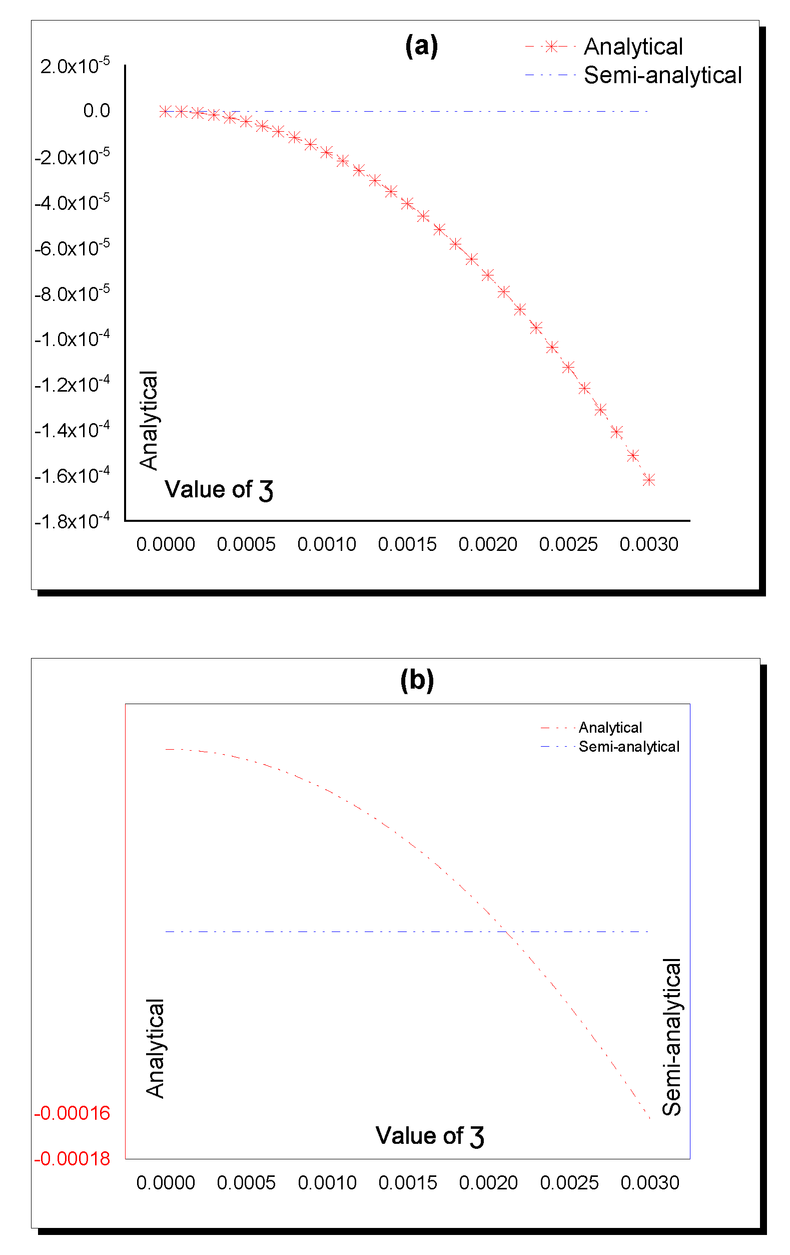
| Value of | Analytical | Semi-Analytical | Absolute Error |
|---|---|---|---|
| 0 | 0 | 0 | 0 |
| 0.0001 | −1.8 | 0 | 1.8 |
| 0.0002 | −7.2 | 0 | 7.2 |
| 0.0003 | −1.62 | 0 | 1.62 |
| 0.0004 | −2.88 | 0 | 2.88 |
| 0.0005 | −4.5 | 0 | 4.5 |
| 0.0006 | −6.47999 | 0 | 6.47999 |
| 0.0007 | −8.81999 | 0 | 8.81999 |
| 0.0008 | −1.152 | 0 | 1.152 |
| 0.0009 | −1.458 | 0 | 1.458 |
| 0.001 | −1.8 | 0 | 1.8 |
| 0.0011 | −2.17799 | 0 | 2.17799 |
| 0.0012 | −2.59199 | 0 | 2.59199 |
| 0.0013 | −3.04199 | 0 | 3.04199 |
| 0.0014 | −3.52798 | 0 | 3.52798 |
| 0.0015 | −4.04998 | 0 | 4.04998 |
| 0.0016 | −4.60797 | 0 | 4.60797 |
| 0.0017 | −5.20196 | 0 | 5.20196 |
| 0.0018 | −5.83195 | 0 | 5.83195 |
| 0.0019 | −6.49794 | 0 | 6.49794 |
| 0.002 | −7.19992 | 0 | 7.19992 |
| 0.0021 | −7.93791 | 0 | 7.93791 |
| 0.0022 | −8.71189 | 0 | 8.71189 |
| 0.0023 | −9.52187 | 0 | 9.52187 |
| 0.0024 | −0.000103678 | 0 | 0.000103678 |
| 0.0025 | −0.000112498 | 0 | 0.000112498 |
| 0.0026 | −0.000121678 | 0 | 0.000121678 |
| 0.0027 | −0.000131217 | 0 | 0.000131217 |
| 0.0028 | −0.000141117 | 0 | 0.000141117 |
| 0.0029 | −0.000151377 | 0 | 0.000151377 |
| 0.003 | −0.000161996 | 0 | 0.000161996 |
Publisher’s Note: MDPI stays neutral with regard to jurisdictional claims in published maps and institutional affiliations. |
© 2021 by the authors. Licensee MDPI, Basel, Switzerland. This article is an open access article distributed under the terms and conditions of the Creative Commons Attribution (CC BY) license (https://creativecommons.org/licenses/by/4.0/).
Share and Cite
Khater, M.M.A.; Alabdali, A.M. Faster and Slower Soliton Phase Shift: Oceanic Waves Affected by Earth Rotation. Mathematics 2021, 9, 3223. https://doi.org/10.3390/math9243223
Khater MMA, Alabdali AM. Faster and Slower Soliton Phase Shift: Oceanic Waves Affected by Earth Rotation. Mathematics. 2021; 9(24):3223. https://doi.org/10.3390/math9243223
Chicago/Turabian StyleKhater, Mostafa M. A., and Aliaa Mahfooz Alabdali. 2021. "Faster and Slower Soliton Phase Shift: Oceanic Waves Affected by Earth Rotation" Mathematics 9, no. 24: 3223. https://doi.org/10.3390/math9243223
APA StyleKhater, M. M. A., & Alabdali, A. M. (2021). Faster and Slower Soliton Phase Shift: Oceanic Waves Affected by Earth Rotation. Mathematics, 9(24), 3223. https://doi.org/10.3390/math9243223