Zhang–Zhang Polynomials of Multiple Zigzag Chains Revisited: A Connection with the John–Sachs Theorem

Abstract

Multiple zigzag chains $Z\left(m,n\right)$ of length n and width m constitute an important class of regular graphene flakes of rectangular shape. The physical and chemical properties of these basic pericondensed benzenoids can be related to their various topological invariants, conveniently encoded as the coefficients of a combinatorial polynomial, usually referred to as the ZZ polynomial of multiple zigzag chains $Z\left(m,n\right)$. The current study reports a novel method for determination of these ZZ polynomials based on a hypothesized extension to John–Sachs theorem, used previously to enumerate Kekulé structures of various benzenoid hydrocarbons. We show that the ZZ polynomial of the $Z\left(m,n\right)$ multiple zigzag chain can be conveniently expressed as a determinant of a Toeplitz (or almost Toeplitz) matrix of size $⌈\frac{m}{2}⌉\times ⌈\frac{m}{2}⌉$ consisting of simple hypergeometric polynomials. The presented analysis can be extended to generalized multiple zigzag chains $Z_k\left(m,n\right)$, i.e., derivatives of $Z\left(m,n\right)$ with a single attached polyacene chain of length k. All presented formulas are accompanied by formal proofs. The developed theoretical machinery is applied for predicting aromaticity distribution patterns in large and infinite multiple zigzag chains $Z\left(m,n\right)$ and for computing the distribution of spin densities in biradical states of finite multiple zigzag chains $Z\left(m,n\right)$.

1. Introduction

The construction, enumeration, and characterization of Kekulé structures and Clar covers of benzenoid hydrocarbons constitute one of the most important topics of graph-theoretical characterization of chemical molecules, a scientific discipline dwelling in the intersection of theoretical chemistry and discrete mathematics [1,2,3,4,5]. For a chemist, a Kekulé structure is a resonance structure in which each carbon atoms participates in exactly one double bond [6]. Similarly, a Clar cover is a resonance structure in which each carbon atoms participates in exactly one double bond or in exactly one aromatic sextet with some other five carbon atoms [7]. These concepts are explained graphically in Figure 1 using pyrene (i.e., the multiple zigzag chain structure $Z\left(2,2\right)$) as an example, together with an intuitive definition of the ZZ polynomial of $Z\left(2,2\right)$. For a mathematician, a Kekulé structure K is a spanning subgraph of the molecular graph G corresponding to a given benzenoid $\mathit{B}$, such that every component of K is isomorphic to a complete graph on two vertices, $K_2$. Similarly, a Clar cover C is a spanning subgraph of G, such that every component of C is isomorphic to $K_2$ or isomorphic to a cyclic graph on six vertices, $C_6$ [8]. The most important questions pertinent to graph-theoretical characterization of a given benzenoid $\mathit{B}$ are as follows. (i) What is the number of Kekulé structures, $\mathcal{K}\equiv \mathcal{K}\left(\mathit{B}\right)$, that can be constructed for $\mathit{B}$? (ii) What is the number of Clar covers, $\mathcal{C}\equiv \mathcal{C}\left(\mathit{B}\right)$, that can be constructed for $\mathit{B}$? (iii) What is the maximal number, $Cl\equiv Cl\left(\mathit{B}\right)$, of aromatic sextets $C_6$ that can be accommodated in $\mathit{B}$? (iv) How many distinct Clar covers exist, $c_{Cl}\equiv c_{Cl}\left(\mathit{B}\right)$, with exactly $Cl$ aromatic sextets? (v) Assuming that k is a non-negative integer, how many distinct Clar covers exist, $c_k\equiv c_k\left(\mathit{B}\right)$, with exactly k aromatic sextets? Note that the answer to the last question, i.e., the sequence of numbers $\left[c_0,c_1,c_2,\dots \right]$, is the most general here, being capable of also providing a solution to the preceding questions. Indeed, we have $\mathcal{K}=c_0$, $\mathcal{C}={\sum }_k{c}_k$, $Cl=max\left\{k|c_k\ne 0\right\}$, and $c_{Cl}=c_{max\left\{k|c_k\ne 0\right\}}$. Note that for a finite benzenoid $\mathit{B}$ with N atoms, the maximal number of aromatic sextets that can be accommodated in $\mathit{B}$ is naturally bounded from above by $N/6$, and thus for all $k>N/6$, we have $c_k=0$. The most convenient way of representing the subsequence $\left[c_0,c_1,c_2,\dots ,c_{Cl}\right]$ is given in the form of its generating function

$$\mathrm{ZZ}\left(\mathit{B},x\right)=\sum _{k=0}^{Cl}{c}_k{x}^k,$$

(1)

which is most often referred to as the Clar covering polynomial or, from the names of its inventors, as the Zhang–Zhang polynomial or the ZZ polynomial of $\mathit{B}$ [9,10,11,12,13,14,15]. Substantial research effort has been invested in the determination of $\mathrm{ZZ}\left(\mathit{B},x\right)$ for elementary families of benzenoids [8,16,17,18,19,20,21,22,23,24,25,26,27,28,29,30,31,32,33,34,35,36,37,38,39,40,41]. The rapid development of Clar theory stimulated by these discoveries in recent years has led to many new interesting applications and connections to other branches of chemistry, graph theory, and combinatorics [8,17,18,19,21,28,34,42,43,44,45,46,47,48,49,50,51,52,53,54,55,56,57,58,59,60,61].

In one of our recent contributions to the field of characterization of Clar covers of basic pericondensed benzenoids, we have derived [33] a closed-form generating function for the ZZ polynomials of multiple zigzag chains $Z\left(m,n\right)$ and generalized multiple zigzag chains $Z_k\left(m,n\right)$ [2,62]. For a graphical definition of both families of benzenoids, see Figure 2. For $Z\left(m,n\right)$, the derived formula (Equation (20) of the work in [33]) had an aesthetically pleasing and compact structure of a finite, regular continued fraction

$$\sum _{m=0}^{\infty }\mathrm{ZZ}\left(Z\left(m,n\right),x\right)t^m=\left[0;-t,{\left(-1\right)}^{2}zt,{\left(-1\right)}^{3}zt,\dots ,{\left(-1\right)}^{n}zt,1+{\left(-1\right)}^{n+1}zt\right]$$

(2)

where, as usual in the theory of ZZ polynomials, $z=1+x$, and where the continued fraction notation $\left[a_0;a_1,a_2,a_3,\dots ,a_n\right]$ should be interpreted as in the following example

$$\left[a_0;a_1,a_2,a_3,a_4\right]=a_0+\frac{1}{a_1+\frac{1}{a_2+\frac{1}{a_3+\frac{1}{a_4}}}}$$

(3)

The formula in Equation (2) is quite regular, but probably its high symmetry is most elegantly reflected in a slightly different continued fraction representation:

$$\sum _{m=0}^{\infty }\mathrm{ZZ}\left(Z\left(m,n\right),x\right)t^m=\frac{-1}{\phantom{z}t+\frac{-1}{zt+\frac{-1}{\ddots +\frac{\ddots }{zt+\frac{-1}{zt+\frac{-1}{zt-{\left(-1\right)}^n}}}}}}$$

(4)

Note that the length of the continued fraction in Equation (4) is $n+1$, i.e., the number of times the product $zt$ appears in it is n. Similar expressions, in terms of products of generating functions of the form (4), were obtained for the generalized multiple zigzag chains $Z_k\left(m,n\right)$ shown in Figure 2.

Despite the internal beauty of the $\mathrm{ZZ}\left(Z\left(m,n\right),x\right)$ and $\mathrm{ZZ}\left(Z_k\left(m,n\right),x\right)$ generating functions, it turned out that extracting the original ZZ polynomials from the generating functions in Equations (2) and (4) is a rather formidable task. A binomial expansion of the continued fraction of type (4), starting from the most shallow level, together with an appropriate multiple sum rotation produces a rather lengthy and cumbersome expression for the ZZ polynomial of $Z\left(m,n\right)$ given by

$$\mathrm{ZZ}\left(Z\left(m,n\right),x\right)=\sum _{l_1=0}^m\sum _{l_2=0}^{l_1}\cdots \sum _{l_n=0}^{l_{n-1}}\prod _{j=2}^{n+1}{\left(-1\right)}^{l_j}\left(\genfrac{}{}{0pt}{}{c_j-l_{j-1}}{l_{j-1}-l_j}\right)z^{l_1}$$

(5)

with the coefficient $c_j$ expressed by

$$c_j={\left(-1\right)}^j\left(1+m+2{\displaystyle \sum _{i=1}^{j-2}}{\left(-1\right)}^i{l}_i\right)$$

(6)

Similar expansions for $\mathrm{ZZ}\left(Z_k\left(m,n\right),x\right)$ were not rigorously attempted, in conviction that their mathematical structure is much too complicated and of little practical importance. Equations (5) and (6) provide formally a closed-form formula for $\mathrm{ZZ}\left(Z\left(m,n\right),x\right)$, but at the same time, they do not bring full intellectual satisfaction of possessing such a formula, as Equation (5) provides little, if any, conceptual insight into the problem of enumeration of Clar covers of $Z\left(m,n\right)$. We concluded our previous work [33] by expressing a hope that the evaluation of multiple sums in Equation (5) could lead to a more compact and transparent expression, but to date no such a result has been reported.

In the current work, we report the discovery and demonstrate formal validity of new ZZ polynomial formulas for the multiple zigzag chains $Z\left(m,n\right)$ and the generalized multiple zigzag chains $Z_k\left(m,n\right)$. The new formulas possess both a transparent algebraic form and deep internal structure, which reveal a direct connection to the structural parameters m, n, and k, and offer a possibility for fast and robust determination of the ZZ polynomials in a form of a determinant of $\left(n+2\right)$-diagonal Toeplitz (or almost Toeplitz) matrices of size $⌈\frac{m}{2}⌉\times ⌈\frac{m}{2}⌉$ or $⌈\frac{m+1}{2}⌉\times ⌈\frac{m+1}{2}⌉$. The new formulas are numerically consistent with the previously obtained Equations (5) and (6). In a sense, the reported formulas are a direct conceptual extension of the formulas in Equations (14.34)–(14.36) and Equations (14.38)–(14.39) of the seminal work of Cyvin and Gutman [2], which reported the determinantal John–Sachs expressions for the number of Kekulé structures for $Z\left(m,n\right)$ and $Z_k\left(m,n\right)$. The actual form of the reported Toeplitz matrices reported here originates from an anticipated extension of the John–Sachs theorem to the world of Clar covers. This hypothesized extension encouraged us to recently conduct an intensive search of examples of elementary benzenoids $\mathit{B}$, for which it is possible to construct a generalization of the John–Sachs matrix, whose determinant would be equal to the ZZ polynomial of $\mathit{B}$ and which, upon the evaluation $x=0$, would reduce to the original John–Sachs matrix of $\mathit{B}$. Among other examples given in [63], we have been able to achieve this task for multiple zigzag chains with $n=1$, 2, and 3. Here, we have been able to achieve this goal for general values of the structural parameters m and n for $Z\left(m,n\right)$, as well as for an arbitrary-sized structures $Z_k\left(m,n\right)$. In addition, the somewhat ad hoc derivations of these formulas are accompanied here with a formal mathematical proof of their validity using the usual recurrence relations obeyed simultaneously by the ZZ polynomials of $Z\left(m,n\right)$ and $Z_k\left(m,n\right)$ and the determinants of the discovered Toeplitz matrices.

In the last section of the current manuscript, we present an application of the developed theoretical framework for computing the aromaticity distribution patterns and the biradical spin population patterns in finite and infinite multiple zigzag chains $Z\left(m,n\right)$. These structures, usually referred by physicists as graphene nanoribbons, received considerable attention from the physics community as promising candidates for future nanoelectronics and spintronics [64,65,66,67,68].

2. Preliminaries

To explain our reasoning leading to the discovery of determinantal formulas for the ZZ polynomials of the multiple zigzag chains $Z\left(m,n\right)$ and generalized multiple zigzag chains $Z_k\left(m,n\right)$, we need to start with some formal preliminaries. Assume, like always, that a benzenoid $\mathit{B}$ is a planar graph embedded in a hexagonal lattice. We define a Kekulé structure K of $\mathit{B}$ as a spanning subgraph of $\mathit{B}$ whose components are $K_2$ (i.e., complete graphs on 2 vertices). Similarly, we define a Clar cover C of $\mathit{B}$ as a spanning subgraph of $\mathit{B}$ whose components are either $K_2$ or $C_6$ (i.e., cycle graphs of length 6) [7]. The number of the $C_6$ components in a given Clar cover C will be referred to as the order of this Clar cover. Denoting by $c_k$ the number of distinct Clar covers of order k, the generating function for the sequence $\left[c_0,c_1,c_2,\dots ,c_{Cl}\right]$ is usually referred to as the Clar covering polynomial (or Zhang–Zhang polynomial or ZZ polynomial) of $\mathit{B}$ and is formally defined as

$$\mathrm{ZZ}\left(\mathit{B},x\right)=\sum _{k=0}^{Cl}{c}_k{x}^k,$$

(7)

where the maximal number $Cl$ of the $C_6$ components that can be accommodated within $\mathit{B}$ is referred to as the Clar number of $\mathit{B}$ [9,10,11,12,13,14,15]. In practice, the ZZ polynomial of an arbitrary benzenoid $\mathit{B}$ can be robustly computed using recursive decomposition algorithms [4,20,26] or can be conveniently determined using interface theory of benzenoids [31,39,69,70,71,72]. A useful theoretical tool for finding ZZ polynomials for an arbitrary benzenoid is ZZDecomposer [25,26]. With this program, one can conveniently define a benzenoid using a mouse drawing pad and subsequently use the underlying graph representation of the benzenoid to find its ZZ polynomial, manipulate its Clar covers, and determine its structural similarity to other related benzenoids. ZZDecomposer has been successfully applied to find close-form formulas of ZZ polynomials for numerous families of basic elementary benzenoids [20,22,23,24,25,27,29,30,32,33,34,36,37,63,73,74].

Assume further that the benzenoids $Z\left(m,n\right)$ and $Z_k\left(m,n\right)$ are drawn in a plane in the way shown in Figure 3 with some of their edges oriented vertically. We say that a vertex $p_i$ is a peak, if all its neighbors are located below $p_i$. Similarly, we say that a vertex $v_j$ is a valley, if all its neighbors are located above $v_j$. It is a well-known fact that if the structure $\mathit{B}$ is Kekuléan, and both families of $\mathit{B}=Z\left(m,n\right)$ and $\mathit{B}=Z_k\left(m,n\right)$ possess this quality for any admissible values of the structural parameters m, n, and k, then the number of peaks in $\mathit{B}$ is equal to the number of valleys in $\mathit{B}$; let us denote this number as l. It is clear from Figure 3 that $l=\frac{m}{2}$ for $Z\left(m,n\right)$ with even m, $l=\frac{m+1}{2}$ for $Z\left(m,n\right)$ and $Z_k\left(m,n\right)$ with odd m, and $l=\frac{m+2}{2}$ for $Z_k\left(m,n\right)$ with even m. The next two important concepts are the wetting region of a peak $p_i$, which is defined as a subgraph of $\mathit{B}$ spanned by all the vertices of $\mathit{B}$ that are accessible from $p_i$ by going exclusively downward, and the funnel region of a valley $v_j$, which is defined as a subgraph of $\mathit{B}$ spanned by all the vertices of $\mathit{B}$ that are accessible from $v_j$ by going exclusively upward. Finally, the $p_i\to v_j$ path region is defined as the intersection of the wetting region of $p_i$ and the funnel region of $v_j$. All these concepts [75] are illustrated schematically in Figure 4.

Let us finally denote by $\mathcal{K}\left(p_i\to v_j\right)$ the number of Kekulé structures for the $p_i\to v_j$ path region. Then, for an arbitrary Kekuléan benzenoid $\mathit{B}$ with l peaks $p_1,\dots ,p_l$ and l valleys $v_1,\dots ,v_l$, the John–Sachs matrix $\mathbb{P}\left(\mathit{B}\right)$ is defined as a square, $l\times l$ matrix with elements $P_{ij}=\mathcal{K}\left(p_i\to v_j\right)$. The celebrated John–Sachs theorem (see, for example, Theorem 1 in [76] or Equation (5) in [77]) states that the number of Kekulé structures for $\mathit{B}$ is equal to the determinant of $\mathbb{P}\left(\mathit{B}\right)$,

$$\mathcal{K}\left(\mathit{B}\right)=\left|\mathbb{P}\left(\mathit{B}\right)\right|.$$

(8)

In our recent work [63], we have asked whether the concept of the John–Sachs matrix $\mathbb{P}\left(\mathit{B}\right)$ can be generalized to encompass the theory of Clar covers. The natural extension meant to make the matrix $\mathbb{P}\left(\mathit{B}\right)$ x-dependent, i.e., replacing $P_{ij}=\mathcal{K}\left(p_i\to v_j\right)$ by $P_{ij}=\mathrm{ZZ}\left(p_i\to v_j,x\right)$, does not work, as the determinant of the resulting matrix does not evaluate to the ZZ polynomial of $\mathit{B}$. Notwithstanding, we have discovered that for numerous families of basic benzenoids, it is actually possible to find a generalized John–Sachs matrix ${\mathbb{P}}_{\mathrm{ZZ}}\left(\mathit{B}\right)$ that possesses all the qualities expected for such a generalization:

• The determinant of the John–Sachs matrix $\mathbb{P}\left(\mathit{B}\right)$ is equal to the number of Kekulé structures as stipulated by Equation (8). Similarly, we request that the determinant of the generalized John–Sachs matrix ${\mathbb{P}}_{\mathrm{ZZ}}\left(\mathit{B}\right)$ is equal to the ZZ polynomial of $\mathit{B}$

  $$\left|{\mathbb{P}}_{\mathrm{ZZ}}\left(\mathit{B}\right)\right|=\mathrm{ZZ}\left(\mathit{B},x\right).$$

  (9)
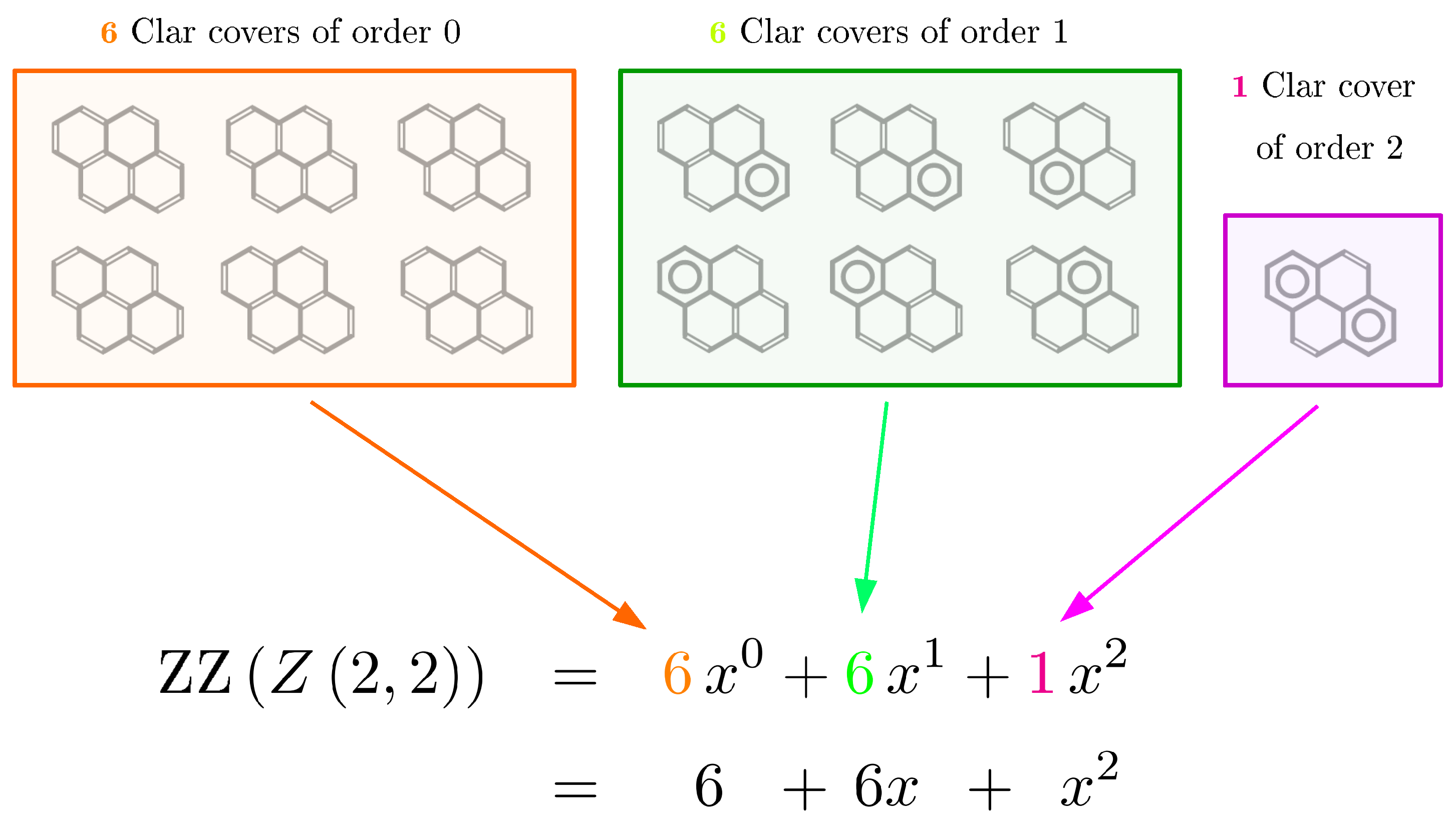
• As the Kekulé structures of $\mathit{B}$ are simply the Clar covers of $\mathit{B}$ of order 0, the number $K\left(\mathit{B}\right)$ of Kekulé structures can be obtained from the ZZ polynomial of $\mathit{B}$ by evaluating it at $x=0$,

  $${\left.\mathrm{ZZ}\left(\mathit{B},x\right)\right|}_{x=0}=\mathcal{K}\left(\mathit{B}\right),$$

  (10)

  which effectively corresponds to removing from the set of Clar covers those which contain at least one component $C_6$. It is then only natural to request that in the same limiting process the John–Sachs path matrix $\mathbb{P}\left(\mathit{B}\right)$ is obtained from the generalized John–Sachs path matrix ${\mathbb{P}}_{\mathrm{ZZ}}\left(\mathit{B}\right)$ upon the evaluation at $x=0$

  $${\left.{\mathbb{P}}_{\mathrm{ZZ}}\left(\mathit{B}\right)\right|}_{x=0}=\mathbb{P}\left(\mathit{B}\right).$$

  (11)

Numerous examples of generalized John–Sachs path matrices ${\mathbb{P}}_{\mathrm{ZZ}}\left(\mathit{B}\right)$ have been given in our recent work [63]. Here, we augment this collection with two further examples corresponding to multiple zigzag chains $Z\left(m,n\right)$ and generalized multiple zigzag chains $Z_k\left(m,n\right)$. Note that most of the previous results were given without a proof, while here for both $Z\left(m,n\right)$ and $Z_k\left(m,n\right)$ we are able to furnish formal proof of all of the presented results. Interestingly, the off-diagonal elements of the generalized John–Sachs path matrices ${\mathbb{P}}_{\mathrm{ZZ}}\left(\mathit{B}\right)$ have a rather unexpected form, for which no plausible explanation nor interpretation has been yet discovered. We hope that a formal extension of the John–Sachs theory to the world of Clar covers will explain this conundrum. We also hope that the results given in the current work will stimulate the community to work on such the generalization of John–Sachs theorem to the world of Clar covers. We finally truly hope that the designed here strategy will be sufficient to discover one of the last missing gems in the theory of ZZ polynomials of basic benzenoids, the ZZ polynomial formula for an arbitrary hexagonal flake $O\left(k,m,n\right)$, similarly like the original John–Sachs theory was used to prove analogous formula for $\mathcal{K}\left(O\left(k,m,n\right)\right)$.

3. Discovery of the Determinantal Formulas

In this section, we briefly discuss the process that led us to the discovery of the determinantal formulas of the ZZ polynomials of multiple zigzag chains $Z\left(m,n\right)$ and generalized multiple zigzag chains $Z_k\left(m,n\right)$. Our motivation for presenting this somewhat obsolete reasoning is purely pedagogical, as it is hoped that similar heuristic reasoning processes can lead to a discovery of other missing formulas in the theory of ZZ polynomials. We limit our discussion to the case of $Z\left(m,n\right)$ with an even value of m. In our previous work [63], we have discovered that the (multiple) zigzag chains $Z\left(m,1\right)$, $Z\left(m,2\right)$, and $Z\left(m,3\right)$ are characterized by the following generalized John–Sachs path matrices:

$$\begin{array}{ccc}\hfill {\mathbb{P}}_{\mathrm{ZZ}}\left(Z\left(m,1\right)\right)& =& \underset{\mathrm{matrix}\frac{m}{2}\times \frac{m}{2}}{\underbrace{\left[\begin{array}{ccccc}{w}_0& w_1& 0& \cdots & 0\\ z& \ddots & \ddots & \ddots & ⋮\\ 0& \ddots & \ddots & \ddots & 0\\ ⋮& \ddots & \ddots & \ddots & w_1\\ 0& \cdots & 0& z& w_0\end{array}\right]}}\mathrm{with}\left\{\begin{array}{ccc}\hfill w_0& =& 1+2z\hfill \\ \hfill w_1& =& z\hfill \end{array}\right.\hfill \end{array}$$

$$\begin{array}{ccc}\hfill {\mathbb{P}}_{\mathrm{ZZ}}\left(Z\left(m,2\right)\right)& =& \underset{\mathrm{matrix}\frac{m}{2}\times \frac{m}{2}}{\underbrace{\left[\begin{array}{ccccc}{w}_0& w_1& w_2& 0& 0\\ z& \ddots & \ddots & \ddots & ⋮\\ 0& \ddots & \ddots & \ddots & w_2\\ ⋮& \ddots & \ddots & \ddots & w_1\\ 0& \cdots & 0& z& w_0\end{array}\right]}}\mathrm{with}\left\{\begin{array}{ccc}\hfill w_0& =& 1+4z+z^2\hfill \\ \hfill w_1& =& 3z\left(1+\frac{2}{3}z\right)\hfill \\ \hfill w_2& =& z^2\hfill \end{array}\right.\hfill \\ \hfill {\mathbb{P}}_{\mathrm{ZZ}}\left(Z\left(m,3\right)\right)& =& \underset{\mathrm{matrix}\frac{m}{2}\times \frac{m}{2}}{\underbrace{\left[\begin{array}{ccccc}{w}_0& w_1& w_2& w_3& 0\\ z& \ddots & \ddots & \ddots & w_3\\ 0& \ddots & \ddots & \ddots & w_2\\ ⋮& \ddots & \ddots & \ddots & w_1\\ 0& \cdots & 0& z& w_0\end{array}\right]}}\mathrm{with}\left\{\begin{array}{ccc}\hfill w_0& =& 1+6z+3z^2\hfill \\ \hfill w_1& =& 6z\left(1+\frac{4}{3}z+\frac{1}{6}{z}^2\right)\hfill \\ \hfill w_2& =& 5z^2\left(1+\frac{2}{5}z\right)\hfill \\ \hfill w_3& =& z^3\hfill \end{array}\right.\hfill \end{array}$$

where, as before, $z=1+x$. A number of regularities can be immediately noticed:

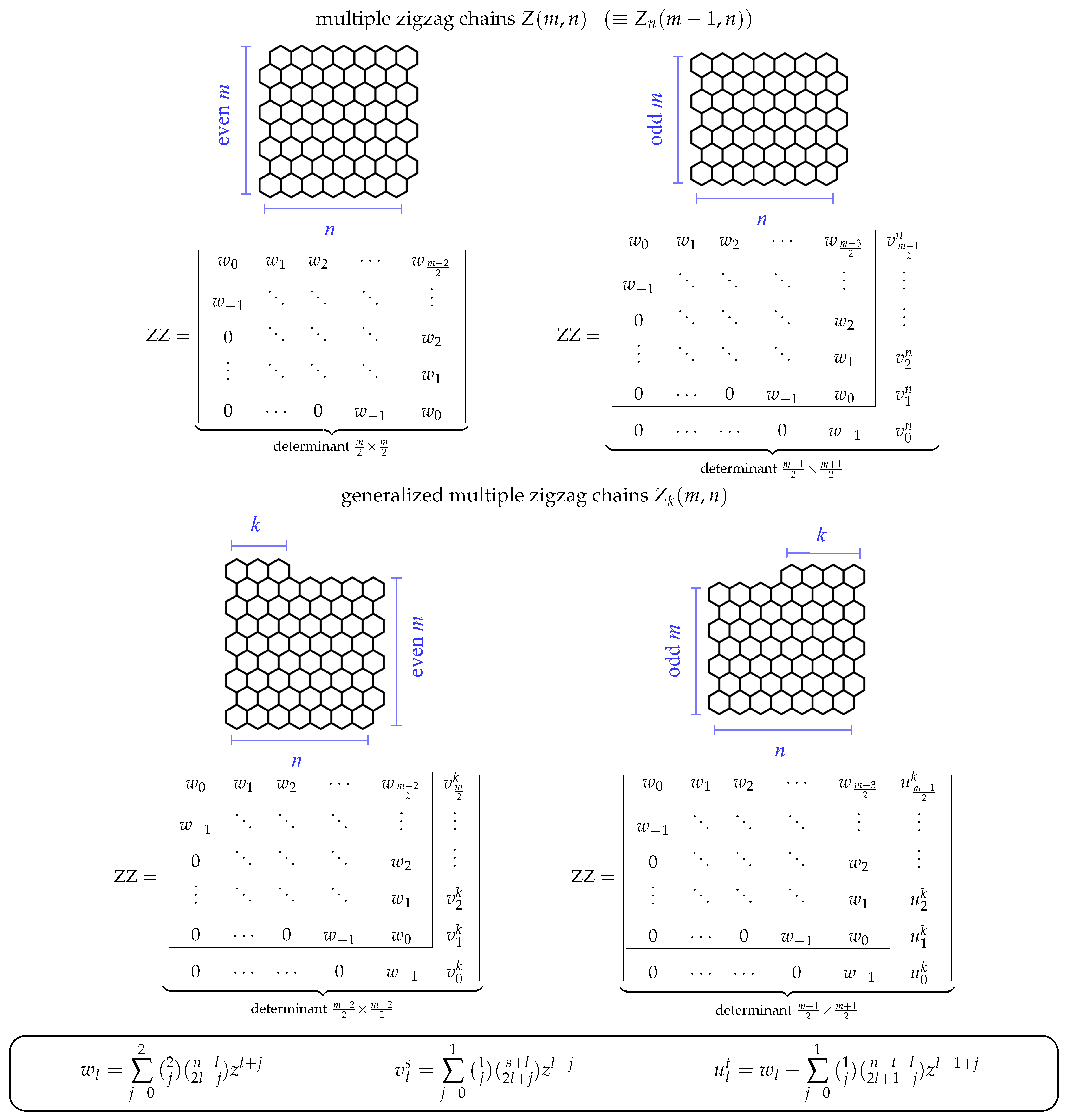
• The matrices ${\mathbb{P}}_{\mathrm{ZZ}}\left(Z\left(m,n\right)\right)$ are $\frac{m}{2}\times \frac{m}{2}$ Toeplitz matrices with $n+2$ diagonals: 1 subdiagonal $\left(z\right)$, 1 diagonal $\left(w_0\right)$, and n consecutive superdiagonals $\left(w_1,\dots ,w_n\right)$.
• The value on the subdiagonal, $z=1+x$, does not depend on n.
• The value of the diagonal element $w_0$ is equal to $\mathrm{ZZ}\left(M\left(2,n\right),x\right)$, given explicitly by

  $$\mathrm{ZZ}\left(M\left(2,n\right),x\right)=\sum _{k=0}^2\left(\genfrac{}{}{0pt}{}{2}{k}\right)\left(\genfrac{}{}{0pt}{}{n}{k}\right)z^k={}_2{F}_1\left[\begin{array}{c}-2,-n\\ 1\end{array};z\right].$$

  (12)
  This value is consistent with the natural extension of the John–Sachs matrix $\mathbb{P}\left(\mathit{B}\right)$ diagonal elements, i.e., with replacing $P_{ii}=\mathcal{K}\left(p_i\to v_i\right)$ by $P_{ii}=\mathrm{ZZ}\left(p_i\to v_i,x\right)$.
• The value $w_l$ on the l-th superdiagonal is a product of a multiplicative factor $z^l$, a numerical factor $c_{nl}$, and a polynomial $p_{nl}\left(z\right)$ of degree 2, 1, or 0.

Further analysis requires slightly larger amount of data. Similar techniques to those used in our previous work [63] allow us to find the values of $w_l$ for ${\mathbb{P}}_{\mathrm{ZZ}}\left(Z\left(m,4\right)\right)$ and ${\mathbb{P}}_{\mathrm{ZZ}}\left(Z\left(m,5\right)\right)$; thus, we have

$$\begin{array}{ccc}\hfill \left\{\begin{array}{ccc}\hfill w_0& =& 1+8z+6z^2\hfill \\ \hfill w_1& =& 10z\left(1+\frac{6}{3}z+\frac{1}{2}{z}^2\right)\hfill \\ \hfill w_2& =& 15z^2\left(1+\frac{4}{5}z+\frac{1}{15}{z}^2\right)\hfill \\ \hfill w_3& =& 7z^3\left(1+\frac{2}{7}z\right)\hfill \\ \hfill w_4& =& z^4\hfill \end{array}\right.& \mathrm{for}& {\mathbb{P}}_{\mathrm{ZZ}}\left(Z\left(m,4\right)\right)\hfill \\ \hfill \left\{\begin{array}{ccc}\hfill w_0& =& 1+10z+10z^2\hfill \\ \hfill w_1& =& 15z\left(1+\frac{8}{3}z+1z^2\right)\hfill \\ \hfill w_2& =& 35z^2\left(1+\frac{6}{5}z+\frac{1}{5}{z}^2\right)\hfill \\ \hfill w_3& =& 28z^2\left(1+\frac{4}{7}z+\frac{1}{28}{z}^2\right)\hfill \\ \hfill w_4& =& 9z^3\left(1+\frac{2}{9}z\right)\hfill \\ \hfill w_5& =& z^5\hfill \end{array}\right.& \mathrm{for}& {\mathbb{P}}_{\mathrm{ZZ}}\left(Z\left(m,5\right)\right)\hfill \end{array}$$

(13)

Equipped with this knowledge it is relatively easy to identify the last two missing pieces of the puzzles: the numerical factor $c_{nl}$ and the polynomial $p_{nl}\left(z\right)$.

• The polynomials $p_{nl}\left(z\right)$ always start from 1 and contain coefficients, which factorize into small primes. This suggests that they are hypergeometric polynomials, i.e., hypergeometric functions ${}_p{F}_q\left[\begin{array}{c}{a}_1,\dots ,a_p\\ b_1,\dots ,b_q\end{array};z\right]$ with at least one of the upper indices $a_j$ being a negative integer. As the formula for the diagonal elements in Equation (12) contains a hypergeometric function ${}_2{F}_1$, it is natural to seek $p_{nl}\left(z\right)$ also in this form. The lower parameter $b_1$ is suggested by the denominator in the linear term of the polynomials $p_{nl}\left(z\right)$, and it is equal to 3 for $w_1$, 5 for $w_2$, 7 for $w_3$, etc. Therefore, in a general case, we can expect for $w_l$ a value of $b_1=1+2l$. Another observation is that the coefficient in the linear term of the polynomial, equal to $\frac{a_1{a}_2}{b_1}$, is always positive, which, taking into account that at least one of the upper indices should be negative, shows that actually both $a_1$ and $a_2$ are negative. One of these numbers, say $a_1$, is immediately recognizable as $-2$, because of the constant degree of the polynomials $p_{nl}\left(z\right)$ for $l\le n-2$. The other index, $a_2$, is a function $a_2=a_2\left(n,l\right)$, which for $l=n$ should be 0 (because of the degree 0 of the polynomial $p_{nl}\left(z\right)$ for $l=n$) and for $l=n-1$ should be 1 (because of the degree 0 of the polynomial $p_{nl}\left(z\right)$ for $l=n$). All these facts suggest that $a_2=l-n$. A straightforward verification with Maple [78] shows that indeed the hypergeometric function ${}_2{F}_1\left[\begin{array}{c}-2,-n+l\\ 1+2l\end{array};z\right]$ reproduces all the reported polynomials $p_{nl}\left(z\right)$ in the matrix elements $w_l$ given above. Note that this polynomial reproduces somewhat fortuitously also the diagonal entry $w_0$.
• The last remaining task is the identification of the two-dimensional sequence of numbers $c_{nl}$, which numerical values for small n and l are given by the following triangle:

  $$\begin{array}{ccc}1\hfill & 1& \phantom{1}1\\ 2\hfill & 1& \phantom{1}3& \phantom{1}1\\ 3\hfill & 1& \phantom{1}6& \phantom{1}5& \phantom{1}1\\ 4\hfill & 1& 10& 15& \phantom{1}7& \phantom{1}1\\ 5\hfill & 1& 15& 35& 28& \phantom{1}9& \phantom{1}1\\ n\mathrm{/}l\hfill & 0& 1& 2& 3& 4& 5\end{array}$$

  (14)
  This task can be readily performed by typing, for example, the last rows of this triangle in the The On-Line Encyclopedia of Integer Sequences [79], which recognizes it as the sequence A085478 generated by

  $$c_{nl}=\left(\genfrac{}{}{0pt}{}{n+l}{2l}\right)\equiv \left(\genfrac{}{}{0pt}{}{n+l}{n-l}\right)$$

  (15)

These two identifications conclude our heuristic deduction and allow to express the ZZ polynomial of multiple zigzag chains $Z\left(m,n\right)$ with even m as a determinant of the generalized John–Sachs path matrix ${\mathbb{P}}_{\mathrm{ZZ}}\left(Z\left(m,n\right)\right)$

$$\mathrm{ZZ}\left(Z\left(m,n\right),x\right)=\left|{\mathbb{P}}_{\mathrm{ZZ}}\left(Z\left(m,n\right)\right)\right|=\underset{\mathrm{determinant}\frac{m}{2}\times \frac{m}{2}}{\underbrace{\left|\begin{array}{ccccc}{w}_0& \cdots & w_n& 0& 0\\ z& \ddots & \phantom{w_m}& \ddots & ⋮\\ 0& \ddots & \ddots & \phantom{w_m}& w_n\\ ⋮& \ddots & \ddots & \ddots & ⋮\\ 0& \cdots & 0& z& w_0\end{array}\right|}},$$

(16)

where the matrix elements $w_l$ are given explicitly by

$$w_l={\left(1+x\right)}^l\left(\genfrac{}{}{0pt}{}{n+l}{n-l}\right){}_2{F}_1\left[\begin{array}{c}-2,-n+l\\ 1+2l\end{array};1+x\right].$$

(17)

The hypergeometric function in Equation (17) can be expanded as a power series in $\left(1+x\right)$, which gives a binomial-like definition convenient for evaluation:

$$w_l=\sum _{j=0}^2\left(\genfrac{}{}{0pt}{}{2}{j}\right)\left(\genfrac{}{}{0pt}{}{n+l}{2l+j}\right){\left(1+x\right)}^{l+j}.$$

(18)

While the definition of $w_l$ given by Equation (18) is probably more transparent and practical, we want to stress that the hypergeometric form in Equation (17) has been essential in the process of the identification of $w_l$, furnishing a convenient unified framework for the search process.

It is further possible to make the form of the matrix ${\mathbb{P}}_{\mathrm{ZZ}}\left(Z\left(m,n\right)\right)$ slightly more uniform by noticing that the presence of the binomial coefficient $\left(\genfrac{}{}{0pt}{}{n+l}{n-l}\right)$ in Equation (17) (or the binomial $\left(\genfrac{}{}{0pt}{}{n+l}{2l+j}\right)$ in Equation (18)) imposes that

$$w_l=0\mathrm{for}l>n,$$

(19)

which means we could omit the triangle of zeros in Equation (16) and simply fill all the superdiagonals with the entries $w_l$. We also note in passing that Equation (18) naturally extends also to $l=-1$, giving

$$w_{-1}=1+x,$$

(20)

which allows to rewrite the entry $z=1+x$ on the first subdiagonal of Equation (16) simply as $w_{-1}$. This gives the most transparent form of the ZZ polynomial of a multiple zigzag chain $Z\left(m,n\right)$ with even m as

$$\mathrm{ZZ}\left(Z\left(m,n\right),x\right)=\left|{\mathbb{P}}_{\mathrm{ZZ}}\left(Z\left(m,n\right)\right)\right|=\underset{\mathrm{determinant}\frac{m}{2}\times \frac{m}{2}}{\underbrace{\left|\begin{array}{ccccc}{w}_0& w_1& w_2& \cdots & w_{\frac{m-2}{2}}\\ w_{-1}& \ddots & \ddots & \ddots & ⋮\\ 0& \ddots & \ddots & \ddots & w_2\\ ⋮& \ddots & \ddots & \ddots & w_1\\ 0& \cdots & 0& w_{-1}& w_0\end{array}\right|}},$$

(21)

where the matrix elements $w_l$ are computed using Equation (18).

The correctness of Equation (16) has been extensively tested by comparing it with the ZZ polynomials of multiple zigzag chains $Z\left(m,n\right)$ computed by brute-force recursive calculations using ZZDecomposer for various values of the structural parameters m and n. A formal proof of correctness of Equation (16) is presented in Section 4.

So far, we have discussed the determinantal formula for the ZZ polynomial of multiple zigzag chains $Z\left(m,n\right)$ with even m. Now, we explain how analogous formulas for $Z_k\left(m,n\right)$ and for $Z\left(m,n\right)$ with odd values of m have been discovered. It is probably simplest to start with $Z_k\left(m,n\right)$ with even m. Figure 3 suggests that for even m, the generalized John–Sachs matrix ${\mathbb{P}}_{\mathrm{ZZ}}\left(Z_k\left(m,n\right)\right)$ corresponds to a matrix of size $\left(\frac{m}{2}+1\right)\times \left(\frac{m}{2}+1\right)$. As, for even values of m, the first $\frac{m}{2}$ peaks and $\frac{m}{2}$ valleys of $Z_k\left(m,n\right)$ coincide with those of $Z\left(m,n\right)$, it is natural to expect that the first, diagonal $\frac{m}{2}\times \frac{m}{2}$ block of ${\mathbb{P}}_{\mathrm{ZZ}}\left(Z_k\left(m,n\right)\right)$ is identical to ${\mathbb{P}}_{\mathrm{ZZ}}\left(Z\left(m,n\right)\right)$. The remaining diagonal entry corresponds to the $\left(p_{\frac{m+2}{2}}\to v_{\frac{m+2}{2}}\right)$ path and according to the hypothesized generalization of the John–Sachs theorem it can be expressed as $\mathrm{ZZ}\left(M\left(1,k\right),x\right)=1+k(1+x)$. It is also natural to assume the value on the first subdiagonal still is $z=1+x$. Discovering the values on the superdiagonals requires intensive numerical experimentation similar in character to the efforts needed to discover $w_l$. Fortunately, this process is relatively straightforward, as independent variations of two structural parameters—k and m—supply a sufficient amount of numerical data to complete the identification in an almost linear fashion. It turns out that the value $v_l^k$ located on the $l^{\mathrm{th}}$ superdiagonal in the last column of ${\mathbb{P}}_{\mathrm{ZZ}}\left(Z_k\left(m,n\right)\right)$ with even m can be expressed by the following hypergeometric formula:

$$v_l^s={\left(1+x\right)}^l\left(\genfrac{}{}{0pt}{}{s+l}{k-l}\right){}_2{F}_1\left[\begin{array}{c}-1,-s+l\\ 1+2l\end{array};1+x\right]$$

(22)

or its binomial-like equivalent

$$v_l^s=\sum _{j=0}^1\left(\genfrac{}{}{0pt}{}{1}{j}\right)\left(\genfrac{}{}{0pt}{}{s+l}{2l+j}\right){\left(1+x\right)}^{l+j},$$

(23)

where $s=k$. Both formulas bear close resemblance to Equations (17) and (18). It is obvious from the presence of the binomial coefficient $\left(\genfrac{}{}{0pt}{}{s+l}{k-l}\right)$ in Equation (22) that

$$v_l^s=0\mathrm{for}l>s,$$

(24)

which means that the last column contains only $k+1$ non-zero entries, including the diagonal element. Somewhat fortuitously, the diagonal element, $v_0^k=1+kz$, can be also expressed by Equations (22) and (23) with $l=0$ and $s=k$.

No effort is needed to discover the form of the generalized John–Sachs matrix ${\mathbb{P}}_{\mathrm{ZZ}}\left(Z\left(m,n\right)\right)$ for $Z\left(m,n\right)$ with odd m; it is immediately identified as ${\mathbb{P}}_{\mathrm{ZZ}}\left(Z_n\left(m-1,n\right)\right)$, because of the structural identity $Z\left(m,n\right)=Z_n\left(m-1,n\right)$.

The last remaining structure, for which we need to find the generalized John–Sachs matrix, is $Z_k\left(m,n\right)$, with an odd value of m. This is a considerable harder task. Here, ${\mathbb{P}}_{\mathrm{ZZ}}\left(Z_k\left(m,n\right)\right)$ corresponds to a matrix of size $\left(\frac{m+1}{2}\right)\times \left(\frac{m+1}{2}\right)$. Again, for odd values of m, the first $\frac{m-1}{2}$ peaks and $\frac{m-1}{2}$ valleys of $Z_k\left(m,n\right)$ coincide with those of $Z\left(m-1,n\right)$, so it is natural to expect that the first, diagonal $\left(\frac{m-1}{2}\right)\times \left(\frac{m-1}{2}\right)$ block of ${\mathbb{P}}_{\mathrm{ZZ}}\left(Z_k\left(m,n\right)\right)$ is identical to ${\mathbb{P}}_{\mathrm{ZZ}}\left(Z\left(m-1,n\right)\right)$. The remaining diagonal element $u_0^k$ corresponds to the $\left\{p_{\frac{m+2}{2}}\to v_{\frac{m+2}{2}}\right\}$ path area, which has a shape of an elementary benzenoid, a ribbon $Rb\left(k,n-k,1,1\right)$, with the ZZ polynomial given by $1+\left(n+k\right)\left(1+x\right)+\frac{k}{2}\left(2n-k-1\right){\left(1+x\right)}^2$. (for details, see Equation (10) in [35]). Extensive numerical experimentation allows to establish that the value $u_l^k$ located on the $l^{\mathrm{th}}$ superdiagonal in the last column of ${\mathbb{P}}_{\mathrm{ZZ}}\left(Z_k\left(m,n\right)\right)$ with odd m can be expressed by

$$u_l^t=v_l^n+\left(1+x\right)\sum _{j=1}^t{v}_l^{n-j}$$

(25)

where $t=k$, with $v_l^n$ and $v_l^{n-j}$ given by Equations (22) or (23). Direct evaluation of Equation (25) gives the following hypergeometric representation of this term:

$$u_l^t={\left(1+x\right)}^l\left(\genfrac{}{}{0pt}{}{n+l}{2l}\right){}_2{F}_1\left[\begin{array}{c}-2,-n+l\\ 1+2l\end{array};1+x\right]-{\left(1+x\right)}^{l+1}\left(\genfrac{}{}{0pt}{}{n-t+l}{2l+1}\right){}_2{F}_1\left[\begin{array}{c}-1,-n+t+l+1\\ 2+2l\end{array};1+x\right]$$

(26)

or its binomial equivalent

$$u_l^t=\sum _{j=0}^2\left(\genfrac{}{}{0pt}{}{2}{j}\right)\left(\genfrac{}{}{0pt}{}{n+l}{2l+j}\right){\left(1+x\right)}^{l+j}-\sum _{j=0}^1\left(\genfrac{}{}{0pt}{}{1}{j}\right)\left(\genfrac{}{}{0pt}{}{n-t+l}{2l+1+j}\right){\left(1+x\right)}^{l+1+j}.$$

(27)

Explicit determinantal formulas for ZZ polynomials of multiple zigzag chains $Z\left(m,n\right)$ and generalized multiple zigzag chains $Z_k\left(m,n\right)$ discovered in the previous paragraphs have been presented in Figure 2 together with binomial representation of all the matrix elements required for their determination and graphical representation of the analyzed structures. Figure 2 can be thought as the graphical abstract of the current work summarizing the most important discoveries reported here. For those who prefer hypergeometric representation of the elements of the relevant path matrices, the following compact formulas should suffice:

$$\begin{array}{ccc}\hfill w_l& =& {\left(1+x\right)}^l\left(\genfrac{}{}{0pt}{}{n+l}{2l}\right){}_2{F}_1\left[\begin{array}{c}-2,-n+l\\ 1+2l\end{array};1+x\right],\hfill \end{array}$$

(28)

$$\begin{array}{ccc}\hfill v_l^s& =& {\left(1+x\right)}^l\left(\genfrac{}{}{0pt}{}{s+l}{2l}\right){}_2{F}_1\left[\begin{array}{c}-1,-s+l\\ 1+2l\end{array};1+x\right],\hfill \end{array}$$

(29)

$$\begin{array}{ccc}\hfill u_l^t& =& w_l-{\left(1+x\right)}^{l+1}\left(\genfrac{}{}{0pt}{}{n-t+l}{2l+1}\right){}_2{F}_1\left[\begin{array}{c}-1,-n+t+l+1\\ 2+2l\end{array};1+x\right].\hfill \end{array}$$

(30)

4. Formal Proof of Determinantal Formulas for $\mathbf{ZZ}\left(\mathit{Z}\left(\mathit{m},\mathit{n}\right),\mathit{x}\right)$ and $\mathbf{ZZ}\left({\mathit{Z}}_{\mathit{k}}\left(\mathit{m},\mathit{n}\right),\mathit{x}\right)$

We start the proof by demonstrating that the formulas presented in Figure 2 produce the ZZ polynomials of $Z\left(m,n\right)$ and $Z_k\left(m,n\right)$ for low values of the index m. We argue in the next paragraph that ZZ polynomials of multiple zigzag chains $Z\left(m,n\right)$ with $m\ge 3$ and ZZ polynomials of generalized multiple zigzag chains $Z_k\left(m,n\right)$ with $m\ge 1$ can be computed in a recursive fashion from analogous ZZ polynomials of $Z\left(m,n\right)$ and $Z_k\left(m,n\right)$ with lower values of the index m. Such a recursive algorithm works neither for $Z\left(m,n\right)$ with $m=1$ or $m=2$ nor for $Z_k\left(m,n\right)$ with $m=0$, so we treat these cases separately here. Simple geometric considerations show that $Z\left(2,n\right)=M\left(2,n\right)$, $Z\left(1,n\right)=M\left(1,n\right)$, and $Z_k\left(0,n\right)=M\left(1,k\right)$. As the ZZ polynomial of a parallelogram $M\left(m,n\right)$ is well known ($\mathrm{ZZ}\left(M\left(m,n\right),x\right)={\sum }_{j=0}^m\left(\genfrac{}{}{0pt}{}{m}{j}\right)\left(\genfrac{}{}{0pt}{}{n}{j}\right){\left(1+x\right)}^j$, see for example Equation (4) of [24]), we obtain the following relations:

$$\mathrm{ZZ}\left(Z\left(1,n\right),x\right)=\mathrm{ZZ}\left(M\left(1,n\right),x\right)=\sum _{j=0}^1\left(\genfrac{}{}{0pt}{}{1}{j}\right)\left(\genfrac{}{}{0pt}{}{n}{j}\right){\left(1+x\right)}^j=v_0^n=\left|{\mathbb{P}}_{\mathrm{ZZ}}\left(Z\left(1,n\right)\right)\right|,$$

(31)

$$\mathrm{ZZ}\left(Z\left(2,n\right),x\right)=\mathrm{ZZ}\left(M\left(2,n\right),x\right)=\sum _{j=0}^2\left(\genfrac{}{}{0pt}{}{2}{j}\right)\left(\genfrac{}{}{0pt}{}{n}{j}\right){\left(1+x\right)}^j=w_0=\left|{\mathbb{P}}_{\mathrm{ZZ}}\left(Z\left(2,n\right)\right)\right|,$$

(32)

$$\mathrm{ZZ}\left(Z_k\left(0,n\right),x\right)=\mathrm{ZZ}\left(M\left(1,k\right),x\right)=\sum _{j=0}^1\left(\genfrac{}{}{0pt}{}{1}{j}\right)\left(\genfrac{}{}{0pt}{}{k}{j}\right){\left(1+x\right)}^j=v_0^k=\left|{\mathbb{P}}_{\mathrm{ZZ}}\left(Z_k\left(0,n\right)\right)\right|,$$

(33)

which confirm that the ZZ polynomials of $Z\left(1,n\right)$, $Z\left(2,n\right)$, and $Z_k\left(0,n\right)$ can be computed from the corresponding generalized John–Sachs matrices presented in Figure 2.

For $Z\left(m,n\right)$ with $m\ge 3$ and for $Z_k\left(m,n\right)$ with $m\ge 1$, the formal proof is a consequence of the general recursive relations derived by Zhang and Zhang for ZZ polynomials. For the multiple zigzag chains $Z\left(m,n\right)$ and generalized multiple zigzag chains $Z_k\left(m,n\right)$, the relevant recursive relations are derived in Figure 5 by choosing a particular edge in $Z\left(m,n\right)$ and $Z_k\left(m,n\right)$ and assigning it to $K_2$, $C_6$, or none. The three possibilities are labeled in Figure 5 as D, R, and S, respectively, where the designated letter abbreviates the corresponding chemical terms: a double bond, an aromatic ring, and a single bond. The resulting recurrence relations interconnecting the ZZ polynomials of various structures $Z\left(m,n\right)$ and $Z_k\left(m,n\right)$

$$\begin{array}{ccc}\hfill \mathrm{ZZ}\left(Z\left(m,n\right),x\right)& =& \mathrm{ZZ}\left(Z_{n-1}\left(m-1,n\right),x\right)+\left(1+x\right)·\mathrm{ZZ}\left(Z\left(m-2,n\right),x\right)\hfill \end{array}$$

(34)

$$\begin{array}{ccc}\hfill \mathrm{ZZ}\left(Z_k\left(m,n\right),x\right)& =& \mathrm{ZZ}\left(Z_{k-1}\left(m,n\right),x\right)+\left(1+x\right)·\mathrm{ZZ}\left(Z_{n-k}\left(m-1,n\right),x\right)\hfill \end{array}$$

(35)

should be consistently satisfied for all the permissible values of the structural parameters m, n, and k. Noting that $Z\left(m,n\right)\equiv Z_0\left(m,n\right)\equiv Z_n\left(m-1,n\right)$, we see that Equation (34) is a specialized version of Equation (35) with $k=n$ and m replaced by $m-1$. It is therefore sufficient to consider only Equation (35), which is valid for the following values of the structural parameters: $1\le m$ and $1\le k\le n$ together with the initial conditions given by Equations (31)–( 33) and corresponding to the edge cases $Z\left(1,n\right)$, $Z\left(2,n\right)$, and $Z_k\left(0,n\right)$. Equipped with this input, we are able to demonstrate below that the deduced earlier determinantal formulas for $\mathrm{ZZ}\left(Z\left(m,n\right),x\right)$ and $\mathrm{ZZ}\left(Z_k\left(m,n\right),x\right)$ (see Figure 2) satisfy the recurrence relation in Equation (35).

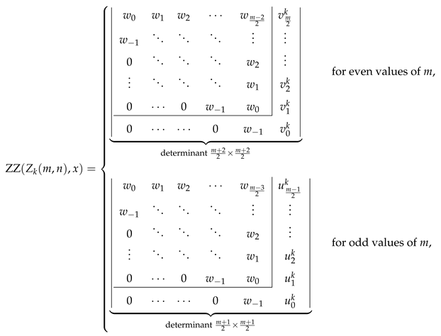
4.1. $Z\left(m,n\right)$ with Even m

Let us compute both sides of Equation (34) assuming the correctness of the determinantal formulas given in Figure 2. LHS of Equation (34) evaluates to $\left|{\mathbb{P}}_{\mathrm{ZZ}}\left(Z\left(m,n\right)\right)\right|$ given by Equation (21). RHS of Equation (34) evaluates to

(36)

where the value of $u_l^{n-1}$ defined in Equation (27) evaluates to the following explicit expression

$$\begin{array}{ccc}\hfill u_l^{n-1}& =& \left\{\begin{array}{cc}{w}_0-\left(1+x\right)\hfill & \mathrm{for}l=0,\hfill \\ w_l\hfill & \mathrm{for}l>0.\hfill \end{array}\right.\hfill \end{array}$$

(37)

Substituting the values of $u_l$ given by Equation (37) to the first determinant in Equation (36) and splitting it with respect to the last column into a sum of two determinants, (see, for example, in [80]) allows us to rewrite Equation (36) as a sum of $\left|{\mathbb{P}}_{\mathrm{ZZ}}\left(Z\left(m,n\right)\right)\right|$ and

(38)

Laplace expansion of the first determinant in Equation (38) with respect to the last column shows that the both addends in Equation (38) cancel each other, retaining only $\left|{\mathbb{P}}_{\mathrm{ZZ}}\left(Z\left(m,n\right)\right)\right|$ as the evaluation of RHS of Equation (34). This is identical to the LHS of Equation (34), proving the consistency of the determinantal formulas reported here with the recurrence relation in Equation (34) for even m.

4.2. $Z\left(m,n\right)$ with Odd m

The analogous consistency demonstration for the $\mathrm{ZZ}\left(Z\left(m,n\right),x\right)$ determinantal formulas with odd m is slightly more complicated. We start with LHS of Equation (34) evaluated to the determinantal form with odd m,

(39)

and perform the following consecutive operations on the following determinant:

• Use $v_l^s$ given by Equation (23) to rewrite the determinant in Equation (39) by expressing its last column as $\mathit{a}+\mathit{b}$, where $\mathit{a}={\left[v_{\frac{m-1}{2}}^n-v_{\frac{m-1}{2}}^{n-1},\dots ,v_1^n-v_1^{n-1},v_0^n-v_0^{n-1}\right]}^{⊺}$ and $\mathit{b}={\left[v_{\frac{m-1}{2}}^{n-1},\dots ,v_1^{n-1},v_0^{n-1}\right]}^{⊺}$.
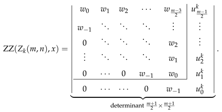
• Decompose the determinant into a sum of two determinants differing only by the last column [80]

  (40)
• Identify $\left(\star \right)$ the second determinant in Equation (40) as $\mathrm{ZZ}\left(Z_{n-1}\left(m-1,n\right),x\right)$ with the help of Figure 2.
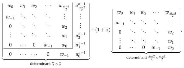
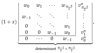
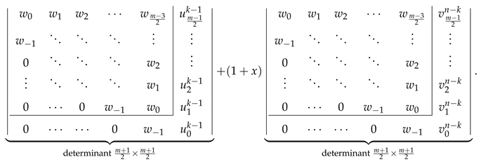
• Rewrite the first determinant in Equation (40) by subtracting its last column from its last-but-one column obtaining

  (41)
• Direct calculations using the definitions in Equations (18) and (23) allow us to establish that

  $$\begin{array}{ccc}\hfill v_0^n-v_0^{n-1}& =& 1+x,\hfill \\ \hfill w_{-1}-v_0^n+v_0^{n-1}& =& 0,\hfill \\ \hfill w_l-v_{l+1}^n+v_{l+1}^{n-1}& =& v_l^n\mathrm{for}l>0.\hfill \end{array}$$
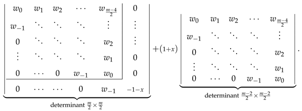
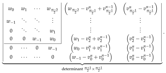
  Using these relations simplifies the determinant in Equation (41) to the following form:

  (42)
• Laplace expansion of the determinant in Equation (42) with respect to the last row gives

  (43)

  allowing us to identify $\left(\star \star \right)$ the expression in Equation (43) as $\left(1+x\right)\mathrm{ZZ}\left(Z\left(m-2,n\right),x\right)$.

The sum of both performed identifications, $\left(\star \right)$ and $\left(\star \star \right)$, is equal to the RHS of Equation (34) evaluated to the determinantal form with odd m; this equality confirms the consistency of the determinantal formulas presented in Figure 2 with Equation (34) for odd m.

4.3. $Z_k\left(m,n\right)$ with Even m

The consistency check process in this case is quite similar to that discussed in the previous section, so we minimize the discussion, giving only its most important intermediate steps. We start with the LHS of Equation (35) evaluated for even m to the determinantal form with the help of Figure 2 obtaining

(44)

We perform the following consecutive operations on this determinant:

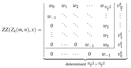
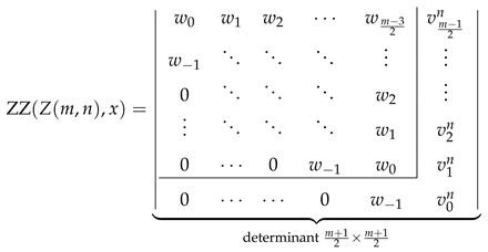
• We rewrite the last column of the determinant in Equation (44) as $\mathit{a}+\mathit{b}$, with $a_l=v_l^k-v_l^{k-1}$ and $b_l=v_l^{k-1}$.
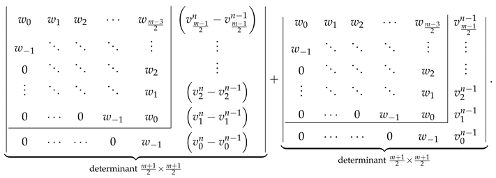
• We decompose the determinant in Equation (44) as a sum of two determinants, the first one having $\mathit{a}$ in the last column and the second one having $\mathit{b}$ in the last column.
• We identify $\left(\star \right)$ the second determinant with the help of Figure 2 as $\mathrm{ZZ}\left(Z_{k-1}\left(m,n\right),x\right)$.
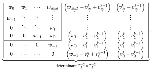
• In the first determinant, we subtract the last column from the last-but-one column obtaining

  (45)
• Direct calculations using the definitions in Equations (18), (23) and (27) allow us to establish that

  $$\begin{array}{ccc}\hfill v_0^k-v_0^{k-1}& =& 1+x,\hfill \\ \hfill w_{-1}-v_0^k+v_0^{k-1}& =& 0,\hfill \\ \hfill w_l-v_{l+1}^k+v_{l+1}^{k-1}& =& u_l^{n-k}\mathrm{for}l>0;\hfill \end{array}$$

  using these relations simplifies the determinant in Equation (45) to the following form:

  (46)
• Laplace expansion of the determinant in Equation (46) with respect to the last row gives

  (47)

  allowing to identify $\left(\star \star \right)$ this expression as $\left(1+x\right)\mathrm{ZZ}\left(Z_{n-k}\left(m-1,n\right),x\right)$.

The sum of both performed identifications, $\left(\star \right)$ and $\left(\star \star \right)$, representing LHS of Equation (35) by construction, is identical to RHS of Equation (35) evaluated to the determinantal form for even m using the formulas presented in Figure 2.

4.4. $Z_k\left(m,n\right)$ with Odd m

The consistency check process in this case relies on the identity $u_l^k=u_l^{k-1}+\left(1+x\right)v_l^{n-k}$ easily derivable directly from the definition of $u_l^k$ given by Equation (25). We start with LHS of Equation (35) evaluated to the determinantal form for odd m with the help of Figure 2, obtaining

(48)

Substituting the aforementioned identity for for every $u_l^k$ in the last column of the determinant in Equation (48) and representing it as a sum of two determinants (decomposition with respect to the last column) gives

(49)

The first determinant in Equation (49) is identified using Figure 2 as $\mathrm{ZZ}\left(Z_{k-1}\left(m,n\right),x\right)$, and the second determinant as $\mathrm{ZZ}\left(Z_{n-k}\left(m-1,n\right),x\right)$. Altogether, the expression in Equation (49) reproduces the RHS of Equation (35) evaluated to the determinantal form for odd m, concluding the consistency check for all possible values (odd and even) of m for both types of structures, $Z\left(m,n\right)$ and $Z_k\left(m,n\right)$, and consequently proving correctness of the determinantal formulas of multiple zigzag chains and generalized multiple zigzag chains given in Figure 2.

5. Chemical Applications

In the current section, we use the derived equations to determine various chemical properties of multiple zigzag chains $Z\left(m,n\right)$. In particular, we focus on the aromaticity pattern distribution within a multiple zigzag chain $Z\left(m,n\right)$ and on the distribution of unpaired spins in biradical excited states of multiple zigzag chains $Z\left(m,n\right)$. First, we define the ZZ aromaticity indicator and the ZZ spin populations and compare them with analogous quantities obtained from rigorous quantum chemical calculations using selected systems. Subsequently, the ZZ indices are computed for families of isostructural multiple zigzag chains and their variation with growing size of the graphene flake is analyzed. The developed ZZ methodology allows one to treat substantially larger flakes than the conventional quantum chemical calculations and in some cases permits computing the asymptotics in transition to infinite graphene nanoribbons.

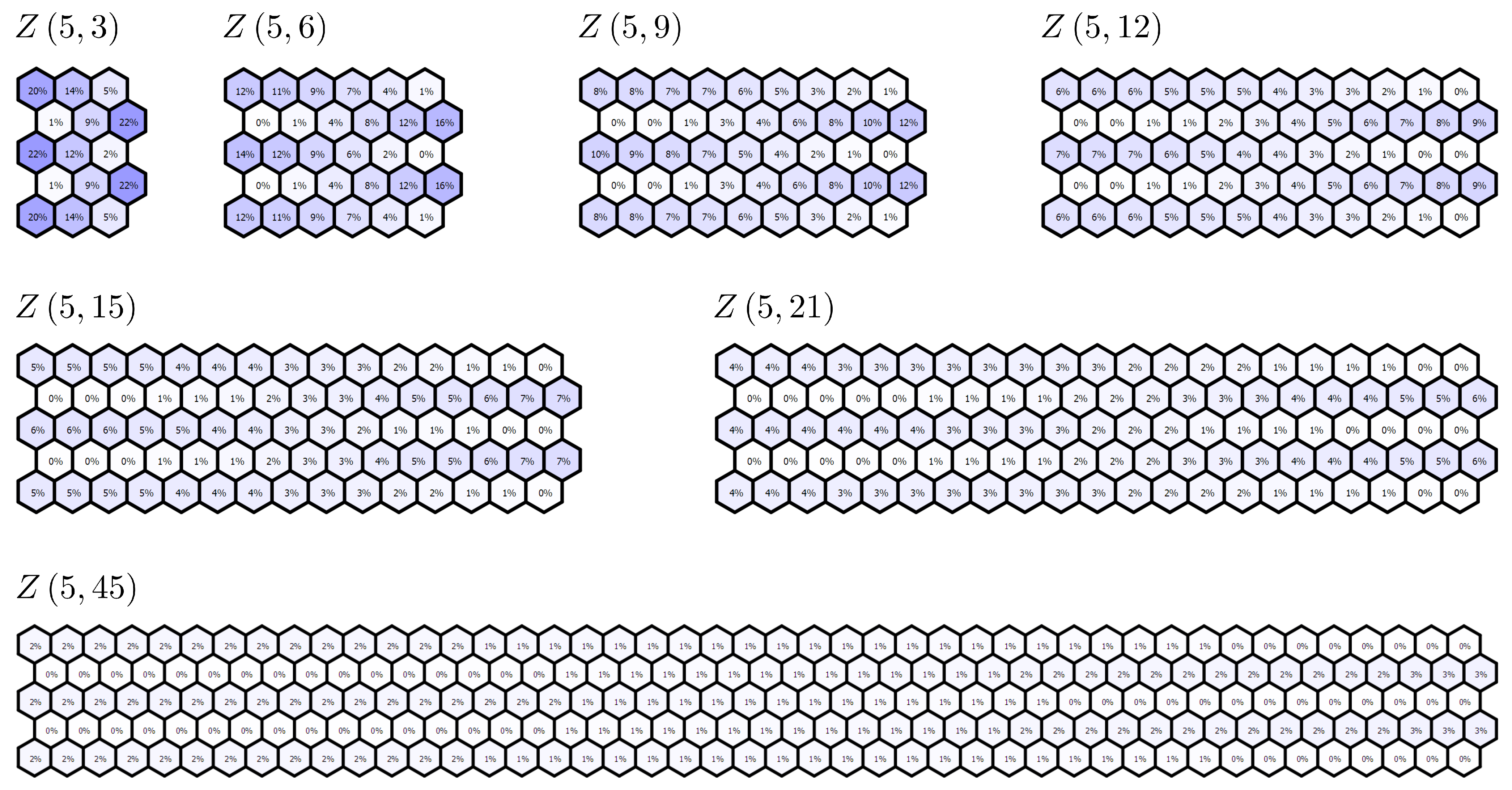
5.1. Local ZZ Aromaticity Indicators for Multiple Zigzag Chains $Z\left(m,n\right)$

The ZZ aromaticity index for some hexagon $h_i$ of a multiple zigzag chain $Z\left(m,n\right)$ is defined as a ratio of the number of Clar covers of $Z\left(m,n\right)$ in which the hexagon $h_i$ has aromatic character to the total number of Clar covers of $Z\left(m,n\right)$. The denominator in this ratio is easily computed as $\mathrm{ZZ}\left(Z\left(m,n\right),1\right)$, while the hexagon-dependent numerators must be computed independently for each hexagon of $Z\left(m,n\right)$. The maximal hexagon aromaticity computed in this way for an arbitrary graphene flake cannot exceed the theoretical value characterizing the infinite graphene sheet, i.e., 33%; the minimal value has a natural lower bound of 0%. The absolute aromaticity scale obtained in this way is very convenient, as it not only allows for finding most and least aromatic hexagons within a given graphene flake, but it also allows for aromaticity comparisons between flakes with various shapes.

The ZZ aromaticity indices computed in this way are shown schematically in Figure 6 for two multiple zigzag chains: $Z\left(5,3\right)$ and $Z\left(4,6\right)$. The maximal ZZ hexagon aromaticity in $Z\left(5,3\right)$ is approximately 67% of the value expected for the infinite graphene sheet, while for $Z\left(4,6\right)$, the maximal value is smaller (45%). A few general observations can be made. (i) Various quantum chemical aromaticity indicators show rather large discrepancies in the predicted aromaticity patterns. In particular, the Bird aromaticity indicator differs substantially from all the other indicators. (ii) The ZZ aromaticity pattern for $Z\left(5,3\right)$ agrees quite well with analogous patterns predicted by HOMA, NICS, PDI, and FLU, i.e., with the majority of selected quantum chemical aromaticity indicators. (iii) The ZZ aromaticity pattern for $Z\left(4,6\right)$ is similar to the patterns predicted by majority of other indicators (NICS, PDI, FLU, SCI, and PLR). (iv) The hexagons with maximal aromaticity in $Z\left(5,3\right)$ and $Z\left(4,6\right)$ are correctly predicted by the ZZ approach. (v) The hexagons with minimal aromaticity (i.e., with maximal antiaromaticity) in $Z\left(5,3\right)$ and $Z\left(4,6\right)$ are again correctly predicted by the ZZ approach. In particular, the ZZ approach is the only one to indicate very clear antiaromatic character of the hexagons characterized by positive chemical shift (blue dots in Figure 6) in the NICS approach. The two benchmark comparisons presented in Figure 6 suggest that the ZZ polynomial approach to graphene flakes aromaticity can be very useful, allowing to treat systems much larger than those accessible with quantum chemical calculations, as the computational cost of computing ZZ polynomials is only fractional in comparison to quantum chemical calculations.

The ZZ approach is now used to study the convergence of the aromaticity patterns for the family of multiple zigzag chains $Z\left(5,n\right)$ with the growing value of n. In Figure 7, we present the computed ZZ aromaticity indicators for all the hexagons of $Z\left(5,n\right)$ with $n=3,6,9,12,15,21$, and 45. A few observations are in place. (i) The aromaticity pattern in $Z\left(5,n\right)$ seems to converge with n to a uniformly non-aromatic infinite graphene strip. (ii) The location of the most aromatic and the most anti-aromatic hexagons is not altered by the elongation of the flake. (iii) In each of the five polyacene chains in $Z\left(5,n\right)$, the aromaticity decreases monotonically from the convex end to the concave end. By studying the recursive decomposition of $Z\left(5,n\right)$, it is possible to derive an analytical formula for the aromaticity of the most aromatic hexagon in each polyacene row. Denoting by $A_k\left(n\right)$ the aromaticity of the most aromatic hexagon in the row k of $Z\left(5,n\right)$, the results of the analysis can be given as follows:

$$\begin{array}{ccc}\hfill A_1\left(n\right)=A_5\left(n\right)& =\hfill & \frac{\mathrm{ZZ}\left(Z_{n-1}\left(3,n\right),1\right)}{\mathrm{ZZ}\left(Z\left(5,n\right),1\right)}\hfill \\ \hfill & =\hfill & \frac{5(10n^4+20n^3+8n^2-2n-3)}{(1+2n)(32n^4+64n^3+68n^2+36n+15)}\hfill \end{array}$$

(50)

$$\begin{array}{ccc}\hfill A_2\left(n\right)=A_4\left(n\right)& =\hfill & \frac{\mathrm{ZZ}\left(Z\left(1,n\right),1\right)·\mathrm{ZZ}\left(Z_{n-1}\left(2,n\right),1\right)}{\mathrm{ZZ}\left(Z\left(5,n\right),1\right)}\hfill \\ \hfill & =\hfill & \frac{5(2n+3){(2n-1)}^2}{(32n^4+64n^3+68n^2+36n+15)}\hfill \end{array}$$

(51)

$$\begin{array}{ccc}\hfill A_3\left(n\right)& =\hfill & \frac{{\left(\mathrm{ZZ}\left(Z_{n-1}\left(1,n\right),1\right)\right)}^2}{\mathrm{ZZ}\left(Z\left(5,n\right),1\right)}\hfill \\ \hfill & =\hfill & \frac{15{(2n^2+2n-1)}^2}{(1+2n)(32n^4+64n^3+68n^2+36n+15)}\hfill \end{array}$$

(52)

Each of these formulas converges like $c/n$ to 0 when $n\to \infty$ with the coefficient c equal to $25/32$ for $A_1\left(n\right)$, $40/32$ for $A_2\left(n\right)$, and $30/32$ for $A_3\left(n\right)$, showing that an infinitely long graphene strip of width 5 is completely non-aromatic, i.e., that all the bonds have either single or double character. At the same time, the formulas show that in each finite nanoribbon $Z\left(5,n\right)$ the most aromatic hexagon is located at the convex end of the second polyacene row. Note that obtaining these conclusions would not be possible directly from quantum chemical calculations without the developed here ZZ polynomial methodology.

5.2. Spin Densities in Biradical Multiple Zigzag Chains $Z\left(5,n\right)$

Another application of the developed here methodology is the computation of spin densities in biradical multiple zigzag chains $Z\left(5,n\right)$. The probability of finding an unpaired electron on the $p_z$ orbital of a selected carbon atom is computed from the associated ZZ polynomial in a similar manner as described above for aromaticities. Namely, we consider all possible distributions of two unpaired electrons in a biradical $Z\left(5,n\right)$ structure by localizing them at the $p_z$ orbitals of two selected carbon atoms—C${}_i$ and C${}_j$, and for each such distribution, we compute the number of Clar covers corresponding to it by evaluating the associated ZZ polynomial at $x=1$ (or equivalently, at $z=2$). This number, divided by the total number of Clar covers in the non-radical $Z\left(5,n\right)$ structure, gives the probability of finding the two unpaired electrons at positions C${}_i$ and C${}_j$ simultaneously. Summing such contributions over all the possible distributions of two unpaired electrons gives the total atomic probabilities of finding an unpaired electron over each carbon atom. The probabilities obtained in this way are then normalized to 1 and the resulting ZZ spin density probability distributions are plotted as red (spin up) and blue (spin down) circles centered at carbon atoms; for more details, see in [92]. The results computed in this manner are plotted in Figure 8 for two families of multiple zigzag chains: $Z\left(5,n\right)$ with $n=4,5,6,7,8,9,10,12,15$ and 21 (upper panel) and $Z\left(m,10\right)$ with $m=4,5,6$ and 7 (lower panel). All the presented spin density distributions look alike and consist of a single ↑ spin wave at one zigzag edge of $Z\left(m,n\right)$ and a single ↓ spin wave at the other zigzag edge of $Z\left(m,n\right)$. The spin densities at the carbon atoms in the interior of $Z\left(m,n\right)$ are negligible, except for the smallest studied here structures. The spin waves at each zigzag edge have no nodal points with the maximum of the distribution located approximately at the middle of the edge. By extrapolating this picture to infinite graphene strips, one can expect that the zigzag edges of the strip will have a constant spin density for each carbon atom located at each zigzag edge, with one side corresponding to spin up, and the other side, to spin down. The resulting spin density pattern is consistent with the predicted previously edge-state magnetism of infinite graphene nanoribbons with zigzag edges, for which it was suggested that the antiferromagnetic state may at some conditions be lower in energy than the nonmagnetic state, leading to spontaneous magnetization of such nanoribbons [64,93,94,95,96,97]. Similar considerations for finite-length nanoribbons did not confirm this effect, suggesting that the ferromagnetic correlation of unpaired electrons at the edge of finite nanoribbons is rather an excited state property [98,99]. Nevertheless, it is remarkable that simple topological considerations performed with Clar covers and ZZ polynomials can lead to similar conclusions as those drawn from sophisticated ab initio quantum mechanical calculations.

6. Conclusions

Inspired by the recently reported collection of generalized John–Sachs matrices ${\mathbb{P}}_{\mathrm{ZZ}}\left(\mathit{B}\right)$ for various classes of elementary aromatic hydrocarbons $\mathit{B}$ [63], which allowed us to express the ZZ polynomial of $\mathit{B}$ simply as $\mathrm{ZZ}\left(\mathit{B},x\right)=\left|{\mathbb{P}}_{\mathrm{ZZ}}\left(\mathit{B}\right)\right|$, we have extended this approach in the current work to two important families of benzenoids: multiple zigzag chains $Z\left(m,n\right)$ and generalized multiple zigzag chains $Z_k\left(m,n\right)$, defined graphically in Figure 2. The extension allowed us to discover compact and simple determinantal formulas for $\mathrm{ZZ}\left(Z\left(m,n\right),x\right)$ and $\mathrm{ZZ}\left(Z_k\left(m,n\right),x\right)$, offering a possibility of considerable simplifications in the process of computation of ZZ polynomials for these two types of structures. The previously known $\mathrm{ZZ}\left(Z\left(m,n\right),x\right)$ formula, reported originally as Equation (58) in [33] and reproduced here as Equation (5), has the form of multiple sums of multiple products of complicated binomials and is too complex to shed light on the structure and classification of Clar covers of $Z\left(m,n\right)$. In contrast, the determinantal formulas reported here hide all the algebraic complexity in the form of a determinant of a very simple object: a highly-structured Toeplitz or almost-Toeplitz matrix. In particular, we have discovered that for multiple zigzag chains $Z\left(m,n\right)$ with even values of the structural parameter m, their ZZ polynomials have particularly transparent form given by

$$\mathrm{ZZ}\left(Z\left(m,n\right),x\right)=\underset{\mathrm{determinant}\frac{m}{2}\times \frac{m}{2}}{\underbrace{\left|\begin{array}{ccccc}{w}_0& w_1& w_2& \cdots & w_{\frac{m-2}{2}}\\ w_{-1}& \ddots & \ddots & \ddots & ⋮\\ 0& \ddots & \ddots & \ddots & w_2\\ ⋮& \ddots & \ddots & \ddots & w_1\\ 0& \cdots & 0& w_{-1}& w_0\end{array}\right|}},$$

(53)

where $w_l$ is a simple polynomial in $\left(1+x\right)$ given explicitly by

$$w_l=\sum _{j=0}^2\left(\genfrac{}{}{0pt}{}{2}{j}\right)\left(\genfrac{}{}{0pt}{}{n+l}{2l+j}\right){\left(1+x\right)}^{l+j}.$$

(54)

Note that $w_l\equiv 0$ for $l>n$, so maximally only the lowest $n+2$ diagonals do not vanish identically. An analogous formula for the ZZ polynomial of multiple zigzag chains $Z\left(m,n\right)$ with odd values of the structural parameter m is only slightly more complicated

(55)

where $v_l^s$ is again a simple polynomial in $\left(1+x\right)$ given explicitly by

$$v_l^s=\sum _{j=0}^1\left(\genfrac{}{}{0pt}{}{1}{j}\right)\left(\genfrac{}{}{0pt}{}{s+l}{2l+j}\right){\left(1+x\right)}^{l+j}.$$

(56)

The corresponding formulas for $\mathrm{ZZ}\left(Z_k\left(m,n\right),x\right)$ closely follow the same pattern; we have

(57)

where $u_l^t$ is again a low-order polynomial in $\left(1+x\right)$ explicitly given by

$$u_l^t=v_l^n+\left(1+x\right)\sum _{j=1}^t{v}_l^{n-j}.$$

(58)

The reported determinantal ZZ polynomial formulas for $Z\left(m,n\right)$ and $Z_k\left(m,n\right)$ also implicitly define the corresponding generalized John–Sachs matrices ${\mathbb{P}}_{\mathrm{ZZ}}\left(Z\left(m,n\right)\right)$ and ${\mathbb{P}}_{\mathrm{ZZ}}\left(Z_k\left(m,n\right)\right)$ for these two families of elementary benzenoids, which upon the evaluation $x=0$ reduce to the regular John–Sachs matrices $\mathbb{P}\left(Z\left(m,n\right)\right)$ and $\mathbb{P}\left(Z_k\left(m,n\right)\right)$ given previously by Equations (14.33)–(14.41) in [2] (see also [62]). We want to stress that in contrast to our earlier work on generalized John–Sachs matrices [63] where most of the discovered facts were only conjectures; here, all the presented results are furnished with appropriate formal proofs. We hope that the presented here results will stimulate the graph-theoretical community to discover further examples of generalized John–Sachs matrices ${\mathbb{P}}_{\mathrm{ZZ}}$ also for other benzenoids, which will pave the road to conception and formulation of the generalization of John–Sachs theorem [75,76,77,100,101,102,103,104,105,106] to the world of Clar covers. We also hope that the presented here techniques will suggest an appropriate line of attack on the most difficult unsolved problem in the theory of ZZ polynomials: discovering the closed-form formula for the ZZ polynomial of hexagonal flake $O\left(k,m,n\right)$ with arbitrary set of parameters [37,41,107].

The developed mathematical machinery of ZZ polynomials for $Z\left(m,n\right)$ and $Z_k\left(m,n\right)$ has been applied to two practical chemical problems: determination of aromaticity patterns in finite and infinite graphene nanoribbons and in the determination of spin populations in biradical states of graphene nanoribbons. These results show good agreement with previously reported quantum chemical data, reproducing similar aromaticity patterns for $Z\left(5,3\right)$ and $Z\left(4,6\right)$ as other, well-established aromaticity indicators and similar antiferromagnetic spin patterns as those obtained from solid state calculations. In contrast to the quantum chemical calculations, the developed here methodology allows for studying the transition from the molecular to crystal regime and establishing that the infinite zigzag ribbons are completely antiaromatic. Note that similar conclusions could not be reached from a standard quantum chemical view point.

References

- Gutman, I. Clar formulas and Kekulé structures. MATCH Commun. Math. Comput. Chem. 1985, 17, 75–90. [Google Scholar]
- Cyvin, S.J.; Gutman, I. Kekulé Structures in Benzenoid Hydrocarbons; Springer: Berlin/Heidelberg, Germany, 1988. [Google Scholar]
- Gutman, I.; Cyvin, S.J. Introduction to the Theory of Benzenoid Hydrocarbons; Springer: Berlin/Heidelberg, Germany, 1989. [Google Scholar]
- Gutman, I.; Furtula, B.; Balaban, A.T. Algorithm for simultaneous calculation of Kekulé and Clar structure counts, and Clar number of benzenoid molecules. Polycycl. Aromat. Compd. 2006, 26, 17–35. [Google Scholar] [CrossRef]
- Zhang, F.J.; Guo, X.F.; Zhang, H.P. Advances of Clar’s aromatic sextet theory and Randić’s conjugated circuit model. Open Org. Chem. J. 2011, 5, 87–111. [Google Scholar] [CrossRef] [Green Version]
- Kekulé, A. Untersuchungen über aromatische Verbindungen Ueber die Constitution der aromatischen Verbindungen. I. Ueber die Constitution der aromatischen Verbindungen. Justus Liebigs Ann. Chem. 1866, 137, 129–196. [Google Scholar] [CrossRef] [Green Version]
- Clar, E. The Aromatic Sextet; Wiley: London, UK, 1972. [Google Scholar]
- Žigert Pleteršek, P. Equivalence of the generalized Zhang–Zhang polynomial and the generalized cube polynomial. MATCH Commun. Math. Comput. Chem. 2018, 80, 215–226. [Google Scholar]
- Zhang, H.P. The Clar covering polynomial of S,T–isomers. MATCH Commun. Math. Comput. Chem. 1993, 29, 189–197. [Google Scholar]
- Zhang, H.P. The Clar formulas of regular t–tier strip benzenoid systems. Syst. Sci. Math. Sci. 1995, 8, 327–337. [Google Scholar]
- Zhang, H.P.; Zhang, F.J. The Clar covering polynomial of hexagonal systems I. Discret. Appl. Math. 1996, 69, 147–167. [Google Scholar] [CrossRef]
- Zhang, F.J.; Zhang, H.P.; Liu, Y.T. The Clar covering polynomial of hexagonal systems II. Chin. J. Chem. 1996, 14, 321–325. [Google Scholar] [CrossRef]
- Zhang, H.P. The Clar covering polynomial of hexagonal systems with an application to chromatic polynomials. Discret. Math. 1997, 172, 163–173. [Google Scholar] [CrossRef] [Green Version]
- Zhang, H.P.; Zhang, F.J. The Clar covering polynomial of hexagonal systems III. Discret. Math. 2000, 212, 261–269. [Google Scholar] [CrossRef] [Green Version]
- Zhang, H.P.; Ji, N.D.; Yao, H.Y. Transfer–matrix calculation of the Clar covering polynomial of hexagonal systems. MATCH Commun. Math. Comput. Chem. 2010, 63, 379–392. [Google Scholar]
- Gutman, I.; Borovićanin, B. Zhang–Zhang polynomial of multiple linear hexagonal chains. Z. Naturforsch. A 2006, 61, 73–77. [Google Scholar] [CrossRef] [Green Version]
- Gojak, S.; Gutman, I.; Radenković, S.; Vodopivec, A. Relating resonance energy with the Zhang–Zhang polynomial. J. Serb. Chem. Soc. 2007, 72, 665–671. [Google Scholar] [CrossRef]
- Guo, Q.Z.; Deng, H.Y.; Chen, D.D. Zhang–Zhang polynomials of cyclo–polyphenacenes. J. Math. Chem. 2009, 46, 347–362. [Google Scholar] [CrossRef]
- Chen, D.D.; Deng, H.Y.; Guo, Q.Z. Zhang–Zhang polynomials of a class of pericondensed benzenoid graphs. MATCH Commun. Math. Comput. Chem. 2010, 63, 401–410. [Google Scholar]
- Chou, C.P.; Witek, H.A. An algorithm and FORTRAN program for automatic computation of the Zhang–Zhang polynomial of benzenoids. MATCH Commun. Math. Comput. Chem. 2012, 68, 3–30. [Google Scholar]
- Xu, L.Q.; Zhang, F.J. On the quasi–ordering of catacondensed hexagonal systems with respective to their Clar covering polynomials. Z. Naturforsch. A 2012, 67, 550–558. [Google Scholar] [CrossRef]
- Chou, C.P.; Witek, H.A. Comment on “Zhang–Zhang polynomials of cyclo-polyphenacenes” by Q. Guo, H. Deng, and D. Chen. J. Math. Chem. 2012, 50, 1031–1033. [Google Scholar] [CrossRef]
- Chou, C.P.; Li, Y.T.; Witek, H.A. Zhang–Zhang polynomials of various classes of benzenoid systems. MATCH Commun. Math. Comput. Chem. 2012, 68, 31–64. [Google Scholar]
- Chou, C.P.; Witek, H.A. Closed–form formulas for the Zhang–Zhang polynomials of benzenoid structures: Chevrons and generalized chevrons. MATCH Commun. Math. Comput. Chem. 2014, 72, 105–124. [Google Scholar]
- Chou, C.P.; Witek, H.A. Determination of Zhang–Zhang polynomials for various classes of benzenoid systems: Non–heuristic approach. MATCH Commun. Math. Comput. Chem. 2014, 72, 75–104. [Google Scholar]
- Chou, C.P.; Witek, H.A. ZZDecomposer: A graphical toolkit for analyzing the Zhang–Zhang polynomials of benzenoid structures. MATCH Commun. Math. Comput. Chem. 2014, 71, 741–764. [Google Scholar]
- Witek, H.A.; Moś, G.; Chou, C.P. Zhang–Zhang polynomials of regular 3– and 4–tier benzenoid strips. MATCH Commun. Math. Comput. Chem. 2015, 73, 427–442. [Google Scholar]
- Berlič, M.; Tratnik, N.; Žigert Pleteršek, P. Equivalence of Zhang–Zhang polynomial and cube polynomial for spherical benzenoid systems. MATCH Commun. Math. Comput. Chem. 2015, 73, 443–456. [Google Scholar]
- Chou, C.P.; Witek, H.A. Two examples for the application of the ZZDecomposer: Zigzag–edge coronoids and fenestrenes. MATCH Commun. Math. Comput. Chem. 2015, 73, 421–426. [Google Scholar]
- Chou, C.P.; Kang, J.S.; Witek, H.A. Closed–form formulas for the Zhang–Zhang polynomials of benzenoid structures: Prolate rectangles and their generalizations. Discret. Appl. Math. 2016, 198, 101–108. [Google Scholar] [CrossRef]
- Langner, J.; Witek, H.A. Connectivity graphs for single zigzag chains and their application for computing ZZ polynomials. Croat. Chem. Acta 2017, 90, 391–400. [Google Scholar] [CrossRef]
- Witek, H.A.; Langner, J.; Moś, G.; Chou, C.P. Zhang–Zhang polynomials of regular 5–tier benzenoid strips. MATCH Commun. Math. Comput. Chem. 2017, 78, 487–504. [Google Scholar]
- Langner, J.; Witek, H.A.; Moś, G. Zhang–Zhang polynomials of multiple zigzag chains. MATCH Commun. Math. Comput. Chem. 2018, 80, 245–265. [Google Scholar]
- Langner, J.; Witek, H.A. Equivalence between Clar covering polynomials of single zigzag chains and tiling polynomials of 2 × n rectangles. Discret. Appl. Math. 2018, 243, 297–303. [Google Scholar] [CrossRef]
- He, B.H.; Chou, C.P.; Langner, J.; Witek, H.A. Zhang-Zhang polynomials of ribbons. Symmetry 2020, 12, 2060. [Google Scholar] [CrossRef]
- Witek, H.A.; Kang, J.S. ZZ polynomials for isomers of (5, 6)-fullerenes Cn with n = 20–50. Symmetry 2020, 12, 1483. [Google Scholar] [CrossRef]
- Witek, H.A.; Langner, J.; Podeszwa, R. Closed-form Formulas for Zhang-Zhang Polynomials of Hexagonal Graphene Flakes O(k,m, n) with k,m = 1–7 and Arbitrary n. MATCH Commun. Math. Comput. Chem. 2021, 86, 165–194. [Google Scholar]
- Langner, J.; Witek, H.A. ZZ Polynomials of Regular m-tier Benzenoid Strips as Extended Strict Order Polynomials of Associated Posets Part 1. Proof of Equivalence. MATCH Commun. Math. Comput. Chem. 2021, submitted. [Google Scholar]
- Langner, J.; Witek, H.A. ZZ Polynomials of Regular m-tier Benzenoid Strips as Extended Strict Order Polynomials of Associated Posets Part 2. Guide to practical computations. MATCH Commun. Math. Comput. Chem. 2021, submitted. [Google Scholar]
- Langner, J.; Witek, H.A. ZZ Polynomials of Regular m-tier Benzenoid Strips as Extended Strict Order Polynomials of Associated Posets Part 3. Compilation of results for m = 1–6. MATCH Commun. Math. Comput. Chem. 2021. submitted. [Google Scholar]
- He, B.H.; Langner, J.; Witek, H.A. Hexagonal flakes as fused parallelograms: A determinantal formula for Zhang-Zhang polynomials of the O(2,m, n) benzenoids. J. Chin. Chem. Soc. 2021. [Google Scholar] [CrossRef]
- Aihara, J.; Makino, M. Constrained Clar formulas of coronoid hydrocarbons. J. Phys. Chem. A 2014, 118, 1258–1266. [Google Scholar] [CrossRef]
- Bašić, N.; Estélyi, I.; Škrekovski, R.; Tratnik, N. On the Clar number of benzenoid graphs. MATCH Commun. Math. Comput. Chem. 2018, 80, 173–188. [Google Scholar]
- Chan, D.W.H.; Xu, S.J.; Nong, G. A linear–time algorithm for computing the complete forcing number and the Clar number of catacondensed hexagonal systems. MATCH Commun. Math. Comput. Chem. 2015, 74, 201–216. [Google Scholar]
- Cruz, R.; Gutman, I.; Rada, J. Convex hexagonal systems and their topological indices. MATCH Commun. Math. Comput. Chem. 2012, 68, 97–108. [Google Scholar]
- Klavžar, S.; Žigert, P.; Gutman, I. Clar number of catacondensed benzenoid hydrocarbons. J. Mol. Struct. Theochem 2002, 586, 235–240. [Google Scholar] [CrossRef]
- Salem, K.; Klavžar, S.; Vesel, A.; Žigert, P. The Clar formulas of a benzenoid system and the resonance graph. Discrete Appl. Math. 2009, 157, 2565–2569. [Google Scholar] [CrossRef] [Green Version]
- Tratnik, N.; Žigert Pleteršek, P. Resonance graphs of fullerenes. ARS Math. Contemp. 2016, 11, 425–435. [Google Scholar] [CrossRef] [Green Version]
- Vesel, A. Fast computation of Clar formula for benzenoid graphs without nice coronenes. MATCH Commun. Math. Comput. Chem. 2014, 71, 717–740. [Google Scholar]
- Ahmadi, M.B.; Farhadi, E.; Khorasani, V.A. On computing the Clar number of a fullerene using optimization techniques. MATCH Commun. Math. Comput. Chem. 2016, 75, 695–701. [Google Scholar]
- Abeledo, H.; Atkinson, G.W. Unimodularity of the Clar number problem. Linear Algebra Appl. 2007, 420, 441–448. [Google Scholar] [CrossRef] [Green Version]
- Ashrafi, A.R.; Amini, K. Relations between Clar structures, Clar covers and sextet-rotations of dendrimer nanostars. Optoelectron. Adv. Mater. 2009, 3, 1076–1079. [Google Scholar]
- Ashrafi, A.R.; Amini, K. Clar structures, Clar covers and Kekulé index of dendrimer nanostars. Optoelectron. Adv. Mater. 2010, 4, 877–880. [Google Scholar]
- Balaban, A.T. Using Clar sextets for two- and three-dimensional aromatic systems. Phys. Chem. Chem. Phys. 2011, 13, 20649–20658. [Google Scholar] [CrossRef]
- Bérczi-Kovács, E.R.; Bernáth, A. The complexity of the Clar number problem and an exact algorithm. J. Math. Chem. 2018, 56, 597–605. [Google Scholar] [CrossRef]
- Carr, J.A.; Wang, X.F.; Ye, D. Packing resonant hexagons in fullerenes. Discret. Optim. 2014, 13, 49–54. [Google Scholar] [CrossRef]
- Chapman, J.; Foos, J.; Hartung, E.J.; Nelson, A.; Williams, A. Pairwise disagreements of Kekulé, Clar, and Fries numbers for benzenoids: A mathematical and computational investigation. MATCH Commun. Math. Comput. Chem. 2018, 80, 186–206. [Google Scholar]
- Hartung, E.J. Clar chains and a counterexample. J. Math. Chem. 2014, 52, 990–1006. [Google Scholar] [CrossRef]
- Salem, K.; Gutman, I. Clar number of hexagonal chains. Chem. Phys. Lett. 2004, 394, 283–286. [Google Scholar] [CrossRef]
- Zhou, S.; Zhang, H.P.; Gutman, I. Relations between Clar structures, Clar covers, and the sextet-rotation tree of a hexagonal system. Discret. Appl. Math. 2008, 156, 1809–1821. [Google Scholar] [CrossRef] [Green Version]
- Zhou, X.Q.; Zhang, H.P. Clar sets and maximum forcing numbers of hexagonal systems. MATCH Commun. Math. Comput. Chem. 2015, 74, 161–174. [Google Scholar]
- Cyvin, S.J.; Cyvin, B.N.; Brunvoll, J.; Gutman, I. Enumeration of Kekulé structures for multiple zigzag chains and related benzenoid hydrocarbons. Z. Naturforsch 1987, 42, 722–730. [Google Scholar] [CrossRef] [Green Version]
- He, B.H.; Langner, J.; Podeszwa, R.; Witek, H.A. Can the John-Sachs theorem be extended to Clar covers? MATCH Commun. Math. Comput. Chem. 2021, 86, 141–163. [Google Scholar]
- Son, Y.W.; Cohen, M.L.; Louie, S.G. Half-metallic graphene nanoribbons. Nature 2006, 444, 347–349. [Google Scholar] [CrossRef] [PubMed] [Green Version]
- Son, Y.W.; Cohen, M.L.; Louie, S.G. Energy Gaps in Graphene Nanoribbons. Phys. Rev. Lett. 2006, 97, 216803. [Google Scholar] [CrossRef] [Green Version]
- Trauzettel, B.; Bulaev, D.; Loss, D.; Burkard, G. Spin qubits in graphene quantum dots. Nat. Phys. 2007, 3, 192–196. [Google Scholar] [CrossRef] [Green Version]
- Yazyev, O.V.; Katsnelson, M.I. Magnetic Correlations at Graphene Edges: Basis for Novel Spintronics Devices. Phys. Rev. Lett. 2008, 100, 047209. [Google Scholar] [CrossRef] [PubMed] [Green Version]
- Soriano, D.; Muñoz-Rojas, F.; Fernández-Rossier, J.; Palacios, J.J. Hydrogenated graphene nanoribbons for spintronics. Phys. Rev. B 2010, 81, 165409. [Google Scholar] [CrossRef] [Green Version]
- Langner, J.; Witek, H.A. Algorithm for generating generalized resonance structures of single zigzag chains based on interface theory. J. Math. Chem. 2018, 56, 1393–1406. [Google Scholar] [CrossRef]
- Langner, J.; Witek, H.A. Interface theory of benzenoids. MATCH Commun. Math. Comput. Chem. 2020, 84, 143–176. [Google Scholar]
- Langner, J.; Witek, H.A. Interface theory of benzenoids: Basic applications. MATCH Commun. Math. Comput. Chem. 2020, 84, 177–215. [Google Scholar]
- Langner, J.; Witek, H.A. Extended strict order polynomial of a poset and fixed elements of linear extensions. Australas. J. Comb. 2021. under review. [Google Scholar]
- Page, A.J.; Chou, C.P.; Pham, B.Q.; Witek, H.A.; Irle, S.; Morokuma, K. Quantum chemical investigation of epoxide and ether groups in graphene oxide and their vibrational spectra. Phys. Chem. Chem. Phys. 2013, 15, 3725–3735. [Google Scholar] [CrossRef]
- Witek, H.A.; Langner, J. Clar covers of overlapping benzenoids: Case of two identically-oriented parallelograms. Symmetry 2020, 12, 1599. [Google Scholar] [CrossRef]
- Gutman, I.; Cyvin, S.J. A new method for the enumeration of Kekulé structures. Chem. Phys. Lett. 1987, 136, 137–140. [Google Scholar] [CrossRef]
- John, P.; Sachs, H. Calculating the numbers of perfect matchings and of spanning trees, Pauling’s orders, the characteristic polynomial, and the eigenvectors of a benzenoid system. Top. Curr. Chem. 1990, 153, 145–179. [Google Scholar]
- He, W.; He, W. P-V matrix and enumeration of Kekulé structures. Theor. Chim. Acta 1989, 75, 389–400. [Google Scholar]
- Maple 16. Maplesoft, a Division of Waterloo Maple Inc.; Maple Is a Trademark of Waterloo Maple Inc.: Waterloo, ON, Canada, 2012.
- The On-Line Encyclopedia of Integer Sequences. Available online: http://oeis.org/A085478 (accessed on 21 January 2021).
- Hogben, L. (Ed.) Handbook of Linear Algebra; Fact 10 in Section 4.1; Chapman & Hall: Boca Raton, FL, USA, 2007. [Google Scholar]
- Schleyer, P.; Maerker, C.; Dransfeld, A.; Jiao, H.; van Eikema Hommes, N.J.R. Nucleus-Independent Chemical Shifts: A Simple and Efficient Aromaticity Probe. J. Am. Chem. Soc. 1996, 118, 6317–6318. [Google Scholar] [CrossRef]
- Kruszewski, J.; Krygowski, T.M. Definition of aromaticity basing on the harmonic oscillator model. Tetrahedron Lett. 1972, 13, 3839–3842. [Google Scholar] [CrossRef]
- Krygowski, T.M. Crystallographic studies of inter- and intramolecular interactions reflected in aromatic character of π-electron systems. J. Chem. Inf. Comput. Sci. 1993, 33, 70–78. [Google Scholar] [CrossRef]
- Bird, C.W. A new aromaticity index and its application to five-membered ring heterocycles. Tetrahedron 1985, 41, 1409–1414. [Google Scholar] [CrossRef]
- Poater, J.; Fradera, X.; Duran, M.; Solá, M. The Delocalization Index as an Electronic Aromaticity Criterion: Application to a Series of Planar Polycyclic Aromatic Hydrocarbons. Chem. Eur. J. 2003, 9, 400–406. [Google Scholar] [CrossRef] [PubMed]
- Giambiagi, M.; de Giambiagi, M.; Mundim, K. Definition of a multicenter bond index. Struct. Chem. 1990, 1, 423–427. [Google Scholar] [CrossRef]
- Sablon, N.; Proft, F.D.; Solá, M.; Geerlings, P. The linear response kernel of conceptual DFT as a measure of aromaticity. Phys. Chem. Chem. Phys. 2012, 14, 3960–3967. [Google Scholar] [CrossRef]
- Fias, S.; Geerlings, P.; Ayers, P.; De Proft, F. σ, π aromaticity and anti-aromaticity as retrieved by the linear response kernel. Phys. Chem. Chem. Phys. 2013, 15, 2882–2889. [Google Scholar] [CrossRef] [PubMed]
- Sablon, N.; Proft, F.D.; Geerlings, P. The linear response kernel of conceptual DFT as a measure of electron delocalization. Chem. Phys. Lett. 2010, 498, 192–197. [Google Scholar] [CrossRef]
- Sablon, N.; Proft, F.D.; Geerlings, P. The linear response kernel: Inductive and resonance effects quantified. J. Phys. Chem. Lett. 2010, 1, 1228–1234. [Google Scholar] [CrossRef]
- Matito, E.; Duran, M.; Solá, M. The aromatic fluctuation index (FLU): A new aromaticity index based on electron delocalization. J. Chem. Phys. 2004, 122, 014109. [Google Scholar] [CrossRef] [Green Version]
- Chen, H. Development of a New Method Based on Clar Covers for Predicting Spin Populations and Aromaticities in Polycyclic Aromatic Hydrocarbons. Master’s Thesis, National Chiao Tung University, Hsinchu, Taiwan, 2019. [Google Scholar]
- Nakada, K.; Fujita, M.; Dresselhaus, G.; Dresselhaus, M.S. Edge state in graphene ribbons: Nanometer size effect and edge shape dependence. Phys. Rev. B 1996, 54, 17954. [Google Scholar] [CrossRef] [Green Version]
- Fujita, M.; Wakabayashi, K.; Nakada, K.; Kusakabe, K. Peculiar localized state at zigzag graphite edge. J. Phys. Soc. Jpn. 1996, 65, 1920–1923. [Google Scholar] [CrossRef] [Green Version]
- Pisani, L.; Chan, J.A.; Montanari, B.; Harrison, N.M. Electronic structure and magnetic properties of graphitic ribbons. Phys. Rev. B 2007, 75, 064418. [Google Scholar] [CrossRef]
- Feldner, H.; Meng, Z.Y.; Lang, T.C.; Assaad, F.F.; Wessel, S.; Honecker, A. Dynamical Signatures of Edge-State Magnetism of Graphene Nanoribbons. Phys. Rev. Lett. 2011, 106, 226401. [Google Scholar] [CrossRef] [PubMed] [Green Version]
- Wang, Z.; Jin, S.; Liu, F. Spatially separated spin carriers in spin-semiconducting graphene nanoribbons. Phys. Rev. Lett. 2013, 111, 096803. [Google Scholar] [CrossRef] [Green Version]
- Culchac, F.J.; Latgé, A.; Costa, A.T. Spin waves in graphene nanoribbon devices. Phys. Rev. B 2012, 86, 115407. [Google Scholar] [CrossRef]
- Luo, M. Topological edge states of a graphene zigzag nanoribbon with spontaneous edge magnetism. Phys. Rev. B 2020, 102, 075421. [Google Scholar] [CrossRef]
- Sachs, H. Perfect matchings in hexagonal systems. Combinatorica 1984, 4, 89–99. [Google Scholar] [CrossRef]
- John, P.; Sachs, H. Calculating the number of perfect matching and Pauling’s bond orders in hexagonal systems whose inner dual is a tree. In Proceedings of the International Conference on Graph Theory, Los Angeles, CA, USA, 6–7 November 1985; pp. 80–91. [Google Scholar]
- John, P.; Rempel, J. Counting perfect matchings in hexagonal systems. In Proceedings of the International Conference on Graph Theory, Eyba, Germany, 1–5 October 1984; pp. 72–84. [Google Scholar]
- John, P.; Sachs, H. Wegesysteme und Linearfaktoren in hexagonalen und quadratischen Systemen. In Graphen in Forschung und Unterricht; Wagner, F.K., Bodendiek, R., Schumacher, H., Walther, G., Eds.; Verlag Barbara Franzbecker: Bad Salzdetfurth, Germany, 1985. [Google Scholar]
- John, P.E.; Sachs, H.; Zernitz, H. Counting perfect matchings in polyominoes with an application to the dimer problem. Appl. Math. 1987, 19, 465–477. [Google Scholar] [CrossRef]
- He, W.; He, W. Peak-Valley Path Method on Benzenoid and Coronoid System. Top. Curr. Chem. 1990, 153, 195–209. [Google Scholar]
- John, P.E.; Sachs, H.; Zheng, M. Kekulé patterns and Clar patterns in bipartite plane graphs. J. Chem. Inf. Comput. Sci. 1995, 35, 1019–1021. [Google Scholar] [CrossRef]
- He, B.H.; Witek, H.A. Clar theory for hexagonal benzenoids with corner defects. MATCH Commun. Math. Comput. Chem. 2020, 86, 121–140. [Google Scholar]
Publisher’s Note: MDPI stays neutral with regard to jurisdictional claims in published maps and institutional affiliations. |
© 2021 by the author. Licensee MDPI, Basel, Switzerland. This article is an open access article distributed under the terms and conditions of the Creative Commons Attribution (CC BY) license (https://creativecommons.org/licenses/by/4.0/).
Share and Cite
Witek, H.A. Zhang–Zhang Polynomials of Multiple Zigzag Chains Revisited: A Connection with the John–Sachs Theorem. Molecules 2021, 26, 2524. https://doi.org/10.3390/molecules26092524
Witek HA. Zhang–Zhang Polynomials of Multiple Zigzag Chains Revisited: A Connection with the John–Sachs Theorem. Molecules. 2021; 26(9):2524. https://doi.org/10.3390/molecules26092524
Chicago/Turabian StyleWitek, Henryk A. 2021. "Zhang–Zhang Polynomials of Multiple Zigzag Chains Revisited: A Connection with the John–Sachs Theorem" Molecules 26, no. 9: 2524. https://doi.org/10.3390/molecules26092524