
Application of Machine Learning Methods to Predict the Air Half-Lives of Persistent Organic Pollutants


Abstract
:
1. Introduction
2. Results
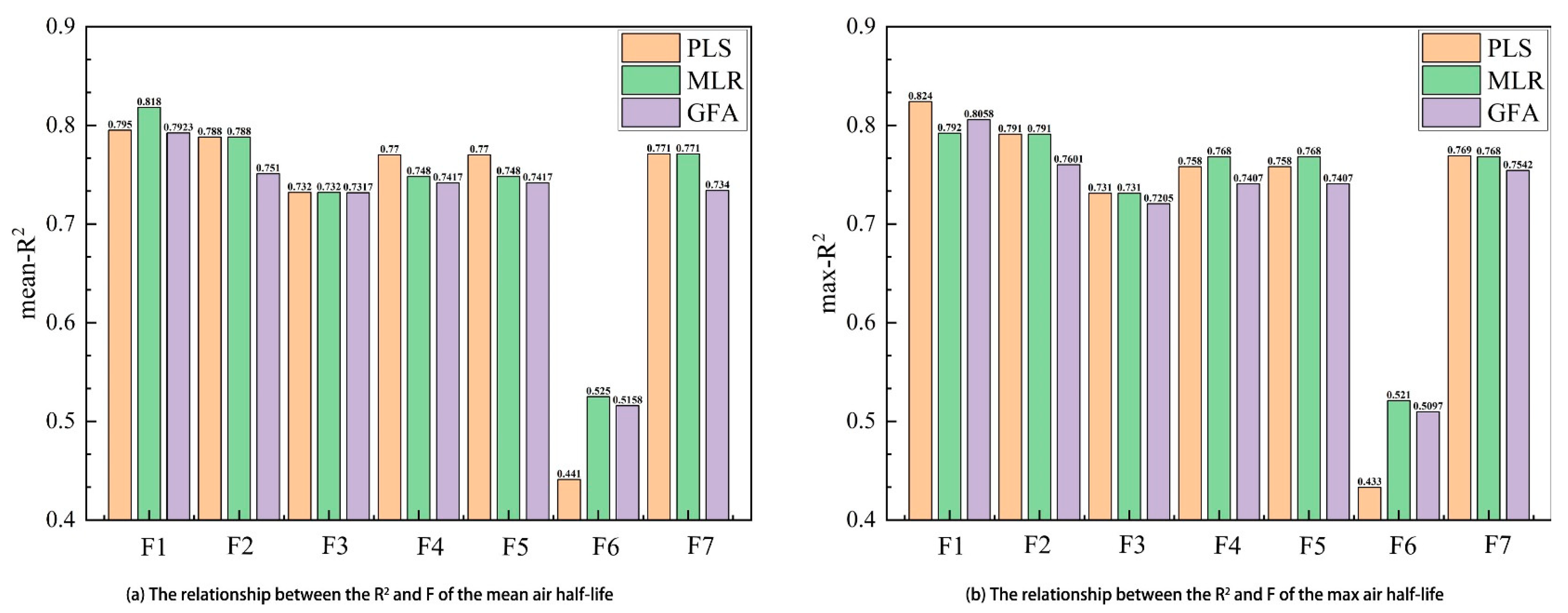
2.1. Dividing the Dataset
2.2. Developing QSAR Models
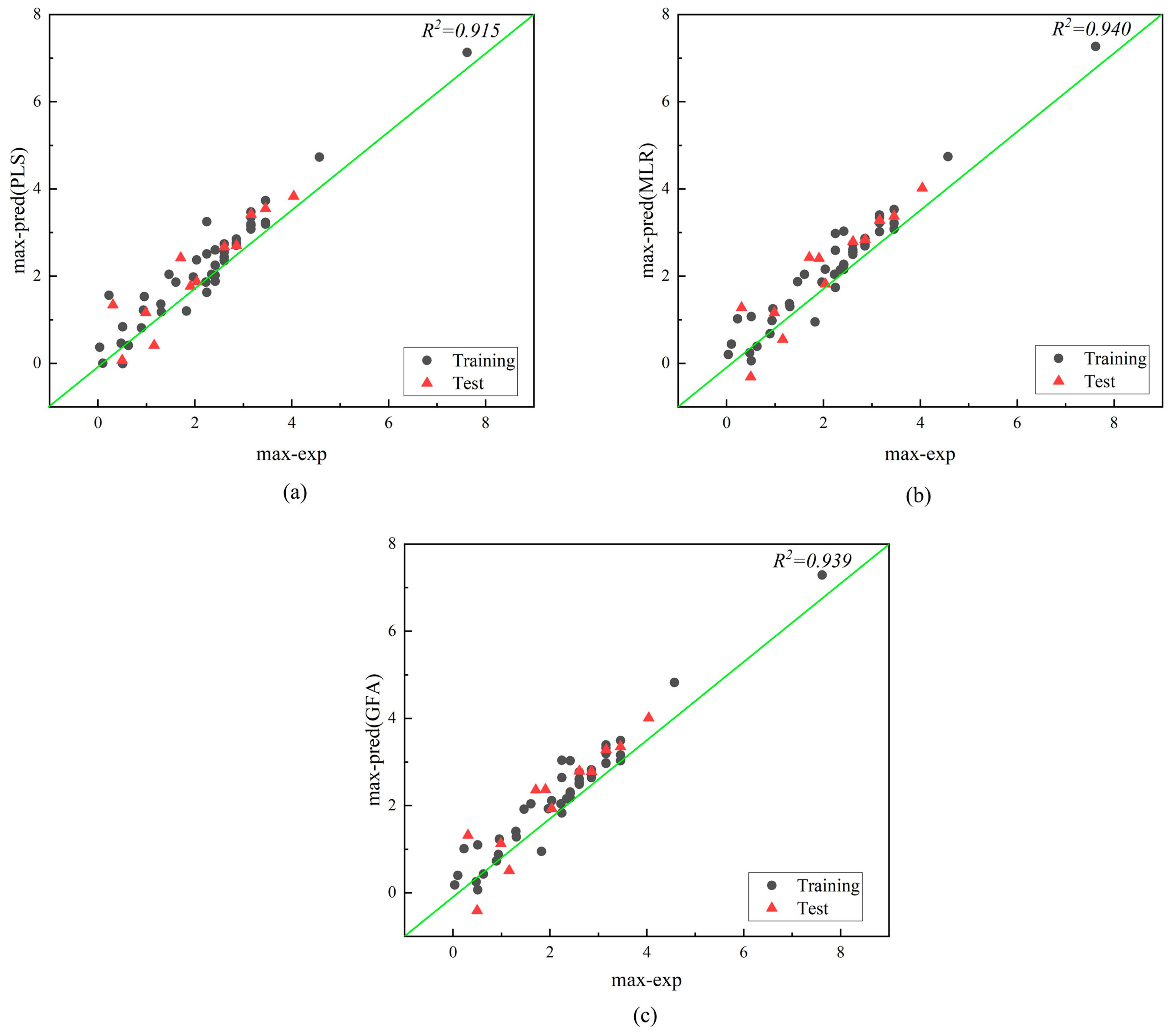
2.2.1. PLS
2.2.2. MLR
2.2.3. GFA
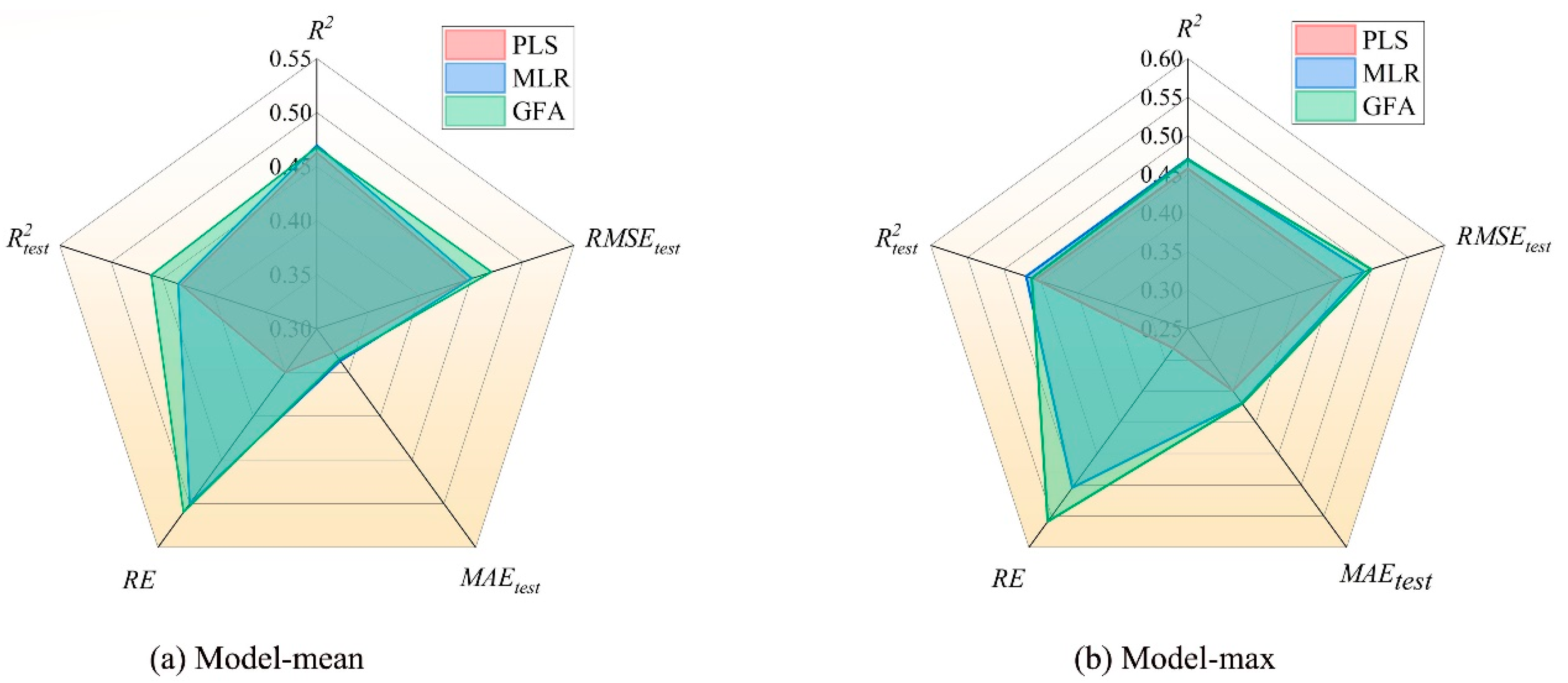
3. Discussion
4. Materials and Methods
4.1. Data Collection and Partitioning
4.2. Calculation and Filtering of Molecular Descriptors
4.3. Machine Learning Methods
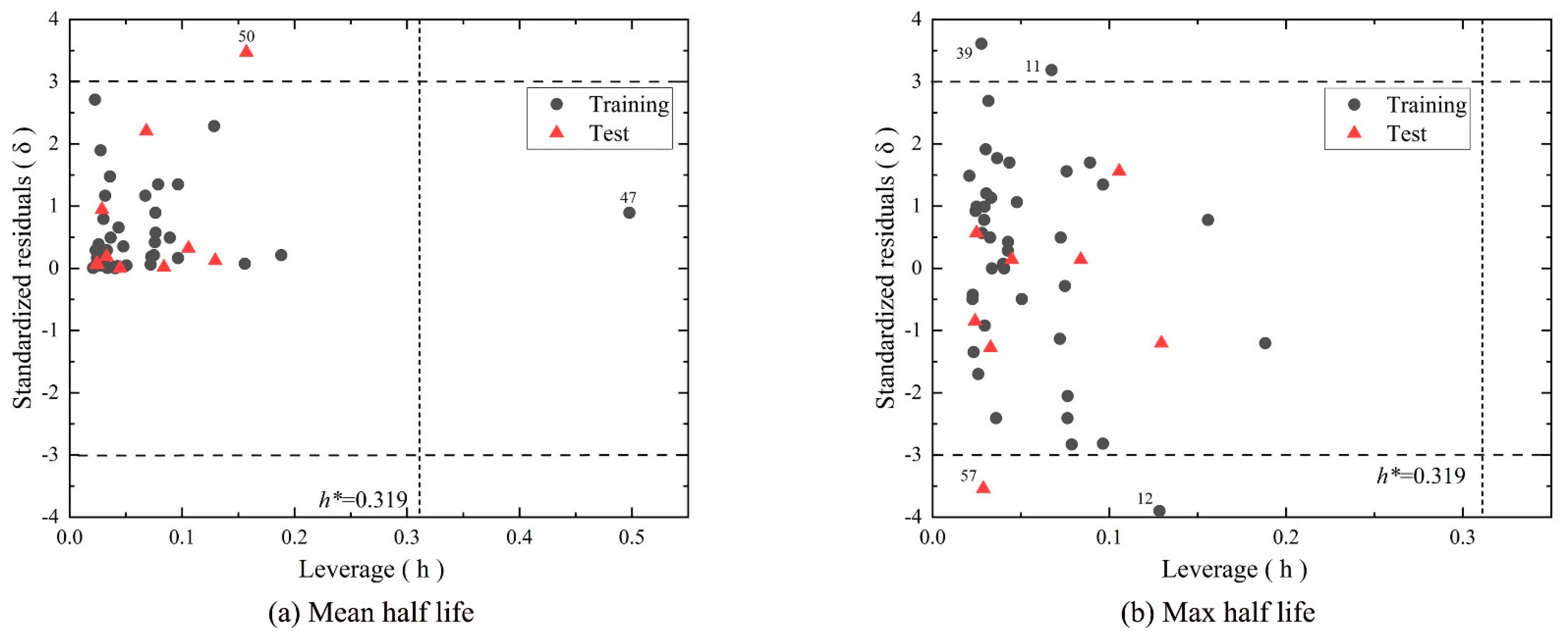
4.4. Model Evaluation and Validation
5. Conclusions
Supplementary Materials
Author Contributions
Funding
Institutional Review Board Statement
Informed Consent Statement
Data Availability Statement
Conflicts of Interest
References
- Watkins, M.; Sizochenko, N.; Rasulev, B.; Leszczynski, J. Estimation of melting points of large set of persistent organic pollutants utilizing QSPR approach. J. Mol. Model. 2016, 22, 1–14. [Google Scholar] [CrossRef]
- Zhang, Q.; Huang, J.; Yu, G. Prediction of soot–water partition coefficients for selected persistent organic pollutants from theoretical molecular descriptors. Prog. Nat. Sci. 2008, 18, 867–872. [Google Scholar] [CrossRef]
- Papa, E.; Gramatica, P. Screening of persistent organic pollutants by QSPR classification models: A comparative study. J. Mol. Graph. Model. 2008, 27, 59–65. [Google Scholar] [CrossRef]
- Puzyn, T.; Gajewicz, A.; Rybacka, A.; Haranczyk, M. Global versus local QSPR models for persistent organic pollutants: Balancing between predictivity and economy. Struct. Chem. 2011, 22, 873–884. [Google Scholar] [CrossRef]
- Zang, Q.; Mansouri, K.; Williams, A.J.; Judson, R.S.; Allen, D.G.; Casey, W.M.; Kleinstreuer, N.C. In silico prediction of physicochemical properties of environmental chemicals using molecular fingerprints and machine learning. J. Chem. Inf. Model. 2017, 57, 36–49. [Google Scholar] [CrossRef] [PubMed]
- Zeng, X.; Wang, Z.; Ge, Z.; Liu, H. Quantitative structure–property relationships for predicting subcooled liquid vapor pressure (PL) of 209 polychlorinated diphenyl ethers (PCDEs) by DFT and the position of Cl substitution (PCS) methods. Atmos. Environ. 2007, 41, 3590–3603. [Google Scholar] [CrossRef]
- Khan, P.M.; Baderna, D.; Lombardo, A.; Roy, K.; Benfenati, E. Chemometric modeling to predict air half-life of persistent organic pollutants (POPs). J. Hazard. Mater. 2020, 382, 121035. [Google Scholar] [CrossRef]
- Wu, Z.; Lei, T.; Shen, C.; Wang, Z.; Cao, D.; Hou, T. ADMET evaluation in drug discovery. 19. Reliable prediction of human cytochrome P450 inhibition using artificial intelligence approaches. J. Chem. Inf. Model. 2019, 59, 4587–4601. [Google Scholar] [CrossRef] [PubMed]
- Jiang, D.; Lei, T.; Wang, Z.; Shen, C.; Cao, D.; Hou, T. ADMET evaluation in drug discovery. 20. Prediction of breast cancer resistance protein inhibition through machine learning. J. Cheminform. 2020, 12, 1–26. [Google Scholar] [CrossRef]
- Xiong, G.L.; Zhao, Y.; Liu, L.; Ma, Z.Y.; Lu, A.P.; Cheng, Y.; Hou, T.J.; Cao, D.S. Computational bioactivity fingerprint similarities to navigate the discovery of novel scaffolds. J. Med. Chem. 2021, 64, 7544–7554. [Google Scholar] [CrossRef] [PubMed]
- Gu, L.; Lu, J.; Li, Q.; Huang, W.; Wu, N.; Yu, Q.; Lu, H.; Zhang, X. Synthesis, extracorporeal nephrotoxicity, and 3D-QSAR of andrographolide derivatives. Chem. Biol. Drug Des. 2021, 97, 592–606. [Google Scholar] [CrossRef] [PubMed]
- Huang, T.; Sun, G.; Zhao, L.; Zhang, N.; Zhong, R.; Peng, Y. Quantitative structure-activity relationship (QSAR) studies on the toxic effects of nitroaromatic compounds (NACs): A systematic review. Int. J. Mol. Sci. 2021, 22, 8557. [Google Scholar] [CrossRef] [PubMed]
- Huang, H.J.; Lee, Y.H.; Chou, C.L.; Zheng, C.M.; Chiu, H.W. Investigation of potential descriptors of chemical compounds on prevention of nephrotoxicity via QSAR approach. Comput. Struct. Biotechnol. J. 2022, 20, 1876–1884. [Google Scholar] [CrossRef]
- Tian, S.; Li, Y.; Wang, J.; Zhang, J.; Hou, T. ADME evaluation in drug discovery. 9. Prediction of oral bioavailability in humans based on molecular properties and structural fingerprints. Mol. Pharm. 2011, 8, 841–851. [Google Scholar] [CrossRef] [PubMed]
- Tian, S.; Sun, H.; Li, Y.; Pan, P.; Li, D.; Hou, T. Development and evaluation of an integrated virtual screening strategy by combining molecular docking and pharmacophore searching based on multiple protein structures. J. Chem. Inf. Model. 2013, 53, 2743–2756. [Google Scholar] [CrossRef] [PubMed]
- Lei, T.; Sun, H.; Kang, Y.; Zhu, F.; Liu, H.; Zhou, W.; Wang, Z.; Li, D.; Li, Y.; Hou, T. ADMET evaluation in drug discovery. 18. Reliable prediction of chemical-induced urinary tract toxicity by boosting machine learning approaches. Mol. Pharm. 2017, 14, 3935–3953. [Google Scholar] [CrossRef] [PubMed]
- Gramatica, P.; Consolaro, F.; Pozzi, S. QSAR approach to POPs screening for atmospheric persistence. Chemosphere 2001, 43, 655–664. [Google Scholar] [CrossRef] [PubMed]
- Zhu, T.; Tao, C. Prediction models with multiple machine learning algorithms for POPs: The calculation of PDMS-air partition coefficient from molecular descriptor. J. Hazard. Mater. 2022, 423, 127037. [Google Scholar] [CrossRef]
- Ashraf, M.A. Persistent organic pollutants (POPs): A global issue, a global challenge. Environ. Sci. Pollut. Res. 2017, 24, 4223–4227. [Google Scholar] [CrossRef]
- Fatemi, M.; Chahi, Z.G. QSPR-based estimation of the half-lives for polychlorinated biphenyl congeners. SAR QSAR Environ. Res. 2012, 23, 155–168. [Google Scholar] [CrossRef]
- Marković, Z.; Filipović, M.; Manojlović, N.; Amić, A.; Jeremić, S.; Milenković, D. QSAR of the free radical scavenging potency of selected hydroxyanthraquinones. Chem. Pap. 2018, 72, 2785–2793. [Google Scholar] [CrossRef]
- Hu, S.; Chen, P.; Gu, P.; Wang, B. A deep learning-based chemical system for QSAR prediction. IEEE J. Biomed. Health Inform. 2020, 24, 3020–3028. [Google Scholar] [CrossRef]
- Pandey, S.K.; Ojha, P.K.; Roy, K. Exploring QSAR models for assessment of acute fish toxicity of environmental transformation products of pesticides (ETPPs). Chemosphere. 2020, 252, 126508. [Google Scholar] [CrossRef]
- Chirico, N.; Gramatica, P. Real external predictivity of QSAR models: How to evaluate it? Comparison of different validation criteria and proposal of using the concordance correlation coefficient. J. Chem. Inf. Model. 2011, 51, 2320–2335. [Google Scholar] [CrossRef] [PubMed]
- Yang, L.; Wang, Y.; Chang, J.; Pan, Y.; Wei, R.; Li, J.; Wang, H. QSAR modeling the toxicity of pesticides against Americamysis bahia. Chemosphere 2020, 258, 127217. [Google Scholar] [CrossRef] [PubMed]
- Adedirin, O.; Uzairu, A.; Shallangwa, G.A.; Abechi, S.E. Optimization of the anticonvulsant activity of 2-acetamido-N-benzyl-2-(5-methylfuran-2-yl) acetamide using QSAR modeling and molecular docking techniques. Beni-Suef. U J. Basic 2018, 7, 430–440. [Google Scholar] [CrossRef]
- Oluwaseye, A.; Uzairu, A.; Shallangwa, G.A.; Abechi, S.E. Quantum chemical descriptors in the QSAR studies of compounds active in maxima electroshock seizure test. J. King Saud Univ. Sci. 2020, 32, 75–83. [Google Scholar] [CrossRef]
- Arthur, D.E.; Soliman, M.E.; Adeniji, S.E.; Adedirin, O.; Peter, F. QSAR and molecular docking study of gonadotropin-releasing hormone receptor inhibitors. Sci. Afr. 2022, 17, e01291. [Google Scholar] [CrossRef]
- De, P.; Roy, K. Nitroaromatics as hypoxic cell radiosensitizers: A 2D-QSAR approach to explore structural features contributing to radiosensitization effectiveness. E J. Med. Chem. Rep. 2022, 4, 100035. [Google Scholar] [CrossRef]
- Kumar, A.; Podder, T.; Kumar, V.; Ojha, P.K. Risk assessment of aromatic organic chemicals to T. pyriformis in environmental protection using regression-based QSTR and Read-Across algorithm. Process Saf. Environ. 2023, 170, 842–854. [Google Scholar] [CrossRef]
- Zhao, Z.; Qin, J.; Gou, Z.; Zhang, Y.; Yang, Y. Multi-task learning models for predicting active compounds. J. Biomed. Inform. 2020, 108, 103484. [Google Scholar] [CrossRef] [PubMed]
- Li, J.; Luo, D.; Wen, T.; Liu, Q.; Mo, Z. Representative feature selection of molecular descriptors in QSAR modeling. J. Mol. Struct. 2021, 1244, 131249. [Google Scholar] [CrossRef]
- Sun, L.; Zhang, M.; Xie, L.; Gao, Q.; Xu, X.; Xu, L. In silico prediction of boiling point, octanol–water partition coefficient, and retention time index of polycyclic aromatic hydrocarbons through machine learning. Chem. Biol. Drug Des. 2023, 101, 52–68. [Google Scholar] [CrossRef]
- Dashtbozorgi, Z.; Golmohammadi, H.; Konoz, E. Support vector regression based QSPR for the prediction of retention time of pesticide residues in gas chromatography–mass spectroscopy. Microchem. J. 2013, 106, 51–60. [Google Scholar] [CrossRef]
- Šaćirović, S.; Jovanović, J.Đ.; Dimić, D.; Petrović, Z.; Simijonović, D.; Manojlović, N.; Antić, M.; Marković, Z. On the origin of the antioxidant potential of selected wines: Combined HPLC, QSAR, and DFT study. Monatsh. Chem. 2021, 152, 1173–1181. [Google Scholar] [CrossRef]
- Krishna, J.G.; Roy, K. QSPR modeling of absorption maxima of dyes used in dye sensitized solar cells (DSSCs). Spectrochim. Acta A Mol. Biomol. Spectrosc. 2022, 265, 120387. [Google Scholar]
- Habicht, J.; Brandenbusch, C.; Sadowski, G. Predicting PC-SAFT pure-component parameters by machine learning using a molecular fingerprint as key input. Fluid Phase Equilibria 2023, 565, 113657. [Google Scholar] [CrossRef]
- Li, F.; Liu, J.; Cao, L. A comparative QSAR study on the estrogenic activities of persistent organic pollutants by PLS and SVM. Emerg. Contam. 2015, 1, 8–13. [Google Scholar] [CrossRef]
- Uyanık, G.K.; Güler, N. A study on multiple linear regression analysis. Procedia Behav. Sci. 2013, 106, 234–240. [Google Scholar] [CrossRef]
- Ly, H.B.; Pham, B.T.; Dao, D.V.; Le, V.M.; Le, L.M.; Le, T.T. Improvement of ANFIS model for prediction of compressive strength of manufactured sand concrete. Appl. Sci. 2019, 9, 3841. [Google Scholar] [CrossRef]
- Sun, L.; Zhang, M.; Xie, L.; Xu, X.; Xu, P.; Xu, L. Computational prediction of Lee retention indices of polycyclic aromatic hydrocarbons by using machine learning. Chem. Biol. Drug Des. 2023, 101, 380–394. [Google Scholar] [CrossRef] [PubMed]
- Qin, L.; Zhang, X.; Chen, Y.; Mo, L.; Zeng, H.; Liang, Y. Predictive QSAR models for the toxicity of disinfection byproducts. Molecules 2017, 22, 1671. [Google Scholar] [CrossRef] [PubMed]


| Molecular Structure Descriptors | |
|---|---|
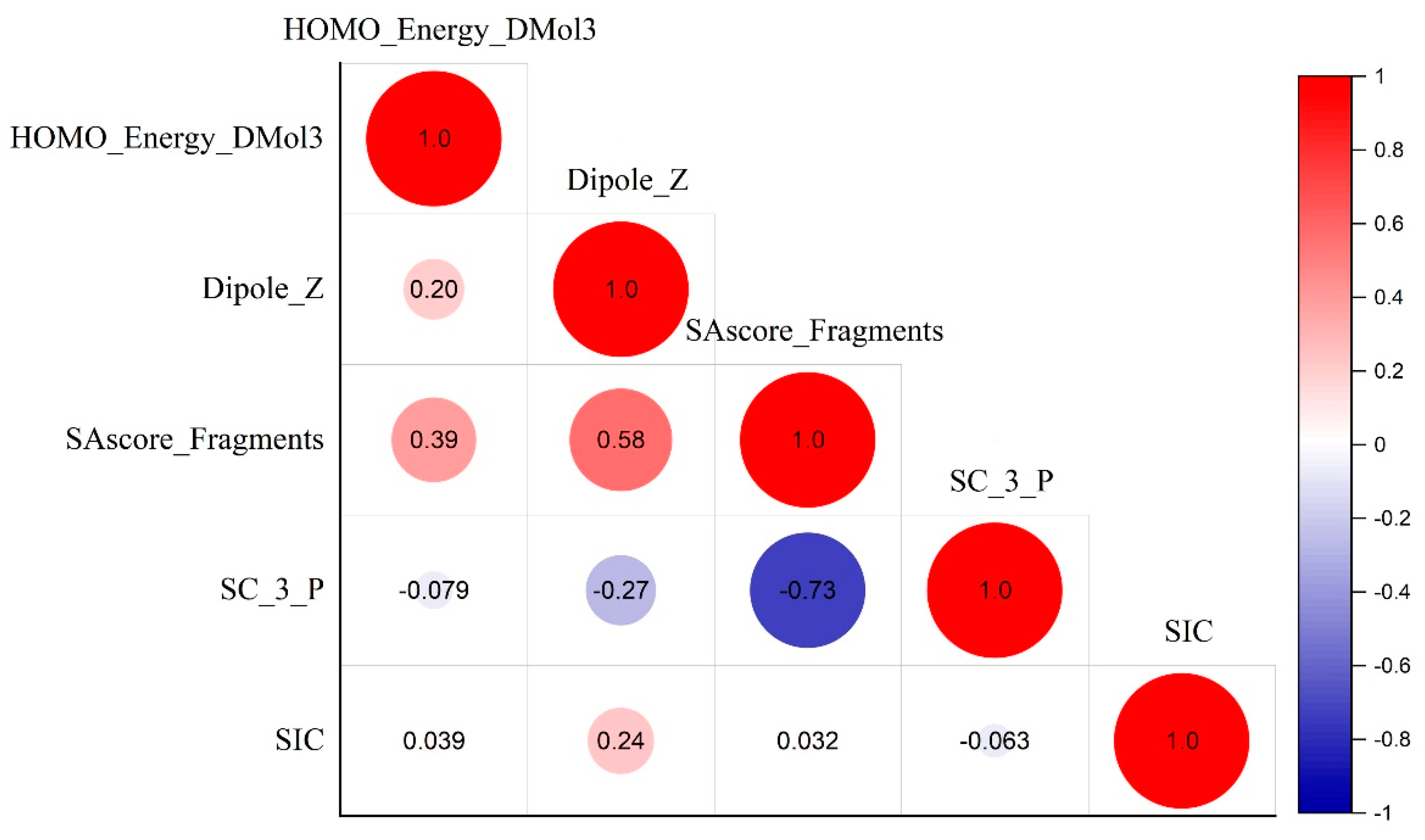
| F1 = 0.05–0.15 | HOMO_Energy_DMol3, Dipole_Z, SAscore_Fragments, SC_3_P, SIC |
| F2 = 0.15–0.3 | HOMO_Energy_DMol3, ES_Sum_aasC, SIC, Num_AtomClasses, Jurs_FNSA_3 |
| F3 = 0.3–0.6 | Num_RingFusionBonds, Jurs_FNSA_3, ES_Sum_aasC, HOMO_Energy_DMol3 |
| F4 = 0.6–0.7 | HOMO_Energy_DMol3, ES_Sum_aasC, Jurs_FNSA_3, SC_3_P, ALogP98 |
| F5 = 0.7–0.8 | HOMO_Energy_DMol3, ES_Sum_aasC, Jurs_FNSA_3, SC_3_P, ALogP98 |
| F6 = 0.8–0.9 | Jurs_FNSA_3, Num_RingFusionBonds, SC_3_P, ALogP98 |
| F7 = 0.9–0.99 | ALogP98, HOMO_Energy_DMol3, Num_AtomClasses, Jurs_FNSA_3, BIC |
| Model | Standard |
|---|---|
| PLS | Cross-validation = five folds; Maximum correlation = 0.7; Dynamic smoothing factor = 0.5; Number of nearest neighbors = 20. |
| MLR | Cross-validation = five folds; Maximum correlation = 0.7; Dynamic smoothing factor = 0.5; Number of nearest neighbors = 20. |
| GFA | The number in the population = 100; The number of iterations = 50,000; Model form = linear; Maximum correlation = 0.7; LOF smoothness parameter = 0.5. |
| Log Mean | |||||||
|---|---|---|---|---|---|---|---|
| Model | R2 | R2text | R2adj | Q2cv | RMSEtest | MAEtest | RE (%) |
| PLS | 0.916 | 0.863 | 0.906 | 0.799 | 0.446 | 0.327 | 3.489 |
| MLR | 0.939 | 0.870 | 0.915 | 0.833 | 0.451 | 0.337 | 5.048 |
| GFA | 0.936 | 0.921 | 0.9006 | / | 0.470 | 0.335 | 5.131 |
| Log Max | |||||||
| Model | R2 | R2text | R2adj | Q2cv | RMSEtest | MAEtest | RE (%) |
| PLS | 0.915 | 0.915 | 0.906 | 0.776 | 0.460 | 0.349 | 5.629 |
| MLR | 0.940 | 0.940 | 0.915 | 0.816 | 0.490 | 0.369 | 10.090 |
| GFA | 0.939 | 0.925 | 0.9026 | / | 0.500 | 0.370 | 11.172 |
| Name | Log Air Half-Life Values (h) | |||||||
|---|---|---|---|---|---|---|---|---|
| Mean-Exp | Mean-Pred | Max-Exp | Max-Pred | |||||
| PLS | MLR | GFA | PLS | MLR | GFA | |||
| Naphtalene | 1.21 | 1.86 | 1.64 | 1.72 | 1.47 | 2.04 | 1.87 | 1.92 |
| Acenaphthene | 0.68 | 1.03 | 0.85 | 0.68 | 0.94 | 1.22 | 0.98 | 0.88 |
| Acenaphthylene | −0.14 | −0.23 | 0.21 | 0.15 | 0.10 | 0.00 | 0.44 | 0.40 |
| Fluorene | 1.57 | 1.00 | 0.74 | 0.75 | 1.83 | 1.20 | 0.95 | 0.95 |
| Anthracene | 0.06 | 1.36 | 0.81 | 0.79 | 0.23 | 1.56 | 1.02 | 1.01 |
| Phenanthrene | 1.04 | 1.15 | 1.12 | 1.19 | 1.30 | 1.36 | 1.37 | 1.41 |
| Fluoranthene | 1.05 | 0.97 | 1.11 | 1.06 | 1.31 | 1.18 | 1.30 | 1.28 |
| Pyrene | 0.13 | 1.12 | 1.03 | 1.09 | 0.31 | 1.34 | 1.28 | 1.32 |
| Chrysene | 0.64 | 0.57 | 0.40 | 0.49 | 0.90 | 0.81 | 0.68 | 0.73 |
| Benz[a]anthracene | 0.30 | 0.21 | 0.00 | 0.00 | 0.48 | 0.46 | 0.24 | 0.25 |
| Benzo[b]fluoranthene | 0.90 | 0.16 | 0.35 | 0.27 | 1.16 | 0.41 | 0.55 | 0.51 |
| Benzo[a]pyrene | −0.13 | 0.11 | −0.04 | −0.07 | 0.04 | 0.37 | 0.20 | 0.18 |
| 7,12-Dimethylbenz[a]anthracene | 0.25 | −0.20 | −0.15 | −0.13 | 0.51 | −0.01 | 0.06 | 0.07 |
| 3-Methylcholanthrene | 0.24 | −0.16 | −0.45 | −0.63 | 0.50 | 0.07 | −0.31 | −0.41 |
| Benzo[ghi]perylene | 0.25 | 0.59 | 0.81 | 0.86 | 0.51 | 0.84 | 1.07 | 1.10 |
| Dibenz[a,h]anthracene | 0.37 | 0.14 | 0.11 | 0.18 | 0.63 | 0.41 | 0.39 | 0.43 |
| Biphenyl | 1.77 | 1.72 | 1.56 | 1.76 | 2.04 | 1.87 | 1.82 | 1.93 |
| 2-Chlorobiphenyl | 2.28 | 1.71 | 1.95 | 2.01 | 2.42 | 1.88 | 2.15 | 2.18 |
| 3-Chlorobiphenyl | 2.28 | 1.86 | 2.08 | 2.12 | 2.42 | 2.02 | 2.26 | 2.28 |
| 4-Chlorobiphenyl | 2.28 | 2.09 | 2.06 | 2.15 | 2.42 | 2.25 | 2.27 | 2.31 |
| 2,2’-Dichlorobiphenyl | 2.48 | 2.38 | 2.56 | 2.60 | 2.61 | 2.55 | 2.74 | 2.77 |
| 2,4-Dichlorobiphenyl | 2.48 | 2.27 | 2.41 | 2.34 | 2.61 | 2.44 | 2.55 | 2.51 |
| 2,5-dichlorobiphenyl | 2.48 | 2.18 | 2.43 | 2.36 | 2.61 | 2.35 | 2.57 | 2.53 |
| 3,3’-dichlorobiphenyl | 2.48 | 2.51 | 2.64 | 2.62 | 2.61 | 2.67 | 2.79 | 2.79 |
| 3,4-Dichlorobiphenyl | 2.48 | 2.26 | 2.34 | 2.32 | 2.61 | 2.42 | 2.50 | 2.49 |
| 3,5-Dichlorobiphenyl | 2.48 | 2.19 | 2.45 | 2.44 | 2.61 | 2.36 | 2.61 | 2.60 |
| 4,4’-Dichlorobiphenyl | 2.48 | 2.58 | 2.32 | 2.44 | 2.61 | 2.74 | 2.54 | 2.61 |
| 2,2’,5-Trichlorobiphenyl | 2.72 | 2.57 | 2.55 | 2.47 | 2.86 | 2.75 | 2.69 | 2.64 |
| 2,3’,5-Trichlorobiphenyl | 2.72 | 2.57 | 2.73 | 2.65 | 2.86 | 2.74 | 2.86 | 2.82 |
| 2,4,4’-Trichlorobiphenyl | 2.72 | 2.67 | 2.57 | 2.54 | 2.86 | 2.85 | 2.73 | 2.71 |
| 2,4,5-Trichlorobiphenyl | 2.72 | 2.53 | 2.64 | 2.57 | 2.86 | 2.71 | 2.79 | 2.75 |
| 2,4,6-Trichlorobiphenyl | 2.72 | 2.53 | 2.71 | 2.61 | 2.86 | 2.70 | 2.84 | 2.78 |
| 2,3’,4’-Trichlorobiphenyl | 2.72 | 2.60 | 2.64 | 2.58 | 2.86 | 2.77 | 2.78 | 2.75 |
| 2,2’,3,3’-Tetrachlorobiphenyl | 3.01 | 3.01 | 3.24 | 3.22 | 3.16 | 3.19 | 3.40 | 3.39 |
| 2,2’,4,4’-Tetrachlorobiphenyl | 3.01 | 3.29 | 3.21 | 3.16 | 3.16 | 3.47 | 3.35 | 3.32 |
| 2,2’,5,5’-Tetrachlorobiphenyl | 3.01 | 3.18 | 3.07 | 3.02 | 3.16 | 3.35 | 3.22 | 3.19 |
| 2,2’,5,6’-Tetrachlorobiphenyl | 3.01 | 2.89 | 2.89 | 2.79 | 3.16 | 3.08 | 3.02 | 2.97 |
| 2,2’,6,6’-Tetrachlorobiphenyl | 3.01 | 3.25 | 3.11 | 3.10 | 3.16 | 3.42 | 3.28 | 3.28 |
| 2,3’,4,4’-Tetrachlorobiphenyl | 3.01 | 2.98 | 2.88 | 2.81 | 3.16 | 3.16 | 3.02 | 2.98 |
| 2,2’,3,4,5-Pentachlorobiphenyl | 3.33 | 3.00 | 3.07 | 2.98 | 3.46 | 3.19 | 3.21 | 3.16 |
| 2,2’,3,4,5’-Pentachlorobiphenyl | 3.33 | 3.03 | 2.93 | 2.84 | 3.46 | 3.23 | 3.08 | 3.03 |
| 2,2’,4,5,5’-Pentachlorobiphenyl | 3.33 | 3.37 | 3.24 | 3.18 | 3.46 | 3.55 | 3.38 | 3.35 |
| 2,2’,4,6,6’-Pentachlorobiphenyl | 3.33 | 3.54 | 3.40 | 3.31 | 3.46 | 3.73 | 3.53 | 3.49 |
| Alpha-hexachlorocyclohexane | 1.71 | 1.73 | 1.61 | 1.72 | 1.97 | 1.98 | 1.86 | 1.93 |
| Gamma-hexachlorocyclohexane | 1.71 | 1.73 | 1.61 | 1.72 | 1.97 | 1.98 | 1.86 | 1.93 |
| p,p’-DDT | 1.99 | 3.13 | 2.82 | 2.93 | 2.25 | 3.25 | 2.98 | 3.04 |
| p,p’-DDE | 1.99 | 1.44 | 1.48 | 1.63 | 2.25 | 1.63 | 1.74 | 1.83 |
| p,p’-DDD | 1.99 | 2.38 | 2.44 | 2.53 | 2.25 | 2.51 | 2.59 | 2.64 |
| Chlordane | 1.45 | 2.13 | 2.24 | 2.10 | 1.71 | 2.42 | 2.43 | 2.36 |
| Dieldrin | 1.35 | 1.58 | 1.78 | 1.78 | 1.61 | 1.86 | 2.04 | 2.04 |
| 2,3,7,8-Tetrachloro-dibenzo-p-dioxin | 1.86 | 1.79 | 1.83 | 1.86 | 2.35 | 2.04 | 2.14 | 2.16 |
| 1,2,3,4,7,8-Hexachloro-dibenzo-p-dioxin | 1.77 | 1.48 | 2.13 | 2.06 | 1.91 | 1.77 | 2.41 | 2.37 |
| Pentachlorobenzene | 3.78 | 3.64 | 3.83 | 3.82 | 4.04 | 3.83 | 4.02 | 4.01 |
| Hexachlorobenzene | 4.31 | 4.55 | 4.48 | 4.63 | 4.57 | 4.73 | 4.74 | 4.82 |
| 2,3,7,8-Tetrachloro-dibenzofuran | 2.19 | 2.37 | 2.80 | 2.78 | 2.42 | 2.60 | 3.03 | 3.03 |
| Aldrin | 0.70 | 1.24 | 0.98 | 0.94 | 0.96 | 1.53 | 1.25 | 1.23 |
| Endrin | 1.93 | 1.58 | 1.78 | 1.78 | 2.23 | 1.86 | 2.04 | 2.04 |
| Mirex | 7.33 | 6.91 | 6.98 | 7.03 | 7.62 | 7.13 | 7.27 | 7.29 |
| Toxaphene | 2.00 | 2.17 | 1.97 | 1.86 | 2.04 | 2.37 | 2.16 | 2.10 |
| Heptachloro | 0.73 | 0.86 | 0.86 | 0.82 | 0.99 | 1.16 | 1.16 | 1.13 |
| Species | Designation | Description |
|---|---|---|
| Molecular descriptors | HOMO_Energy_DMol3 | The energy of the highest occupied molecular orbital |
| Dipole_Z | Component of the dipole moment along the z-axis | |
| SAscore_Fragments | Fragment contribution to SAscore | |
| SC_3_P | Subgraph counts | |
| SIC | Structural information content. Graph-theoretical info content descriptor which differentiates molecules according to their size, degree of branching, and flexibility |
Disclaimer/Publisher’s Note: The statements, opinions and data contained in all publications are solely those of the individual author(s) and contributor(s) and not of MDPI and/or the editor(s). MDPI and/or the editor(s) disclaim responsibility for any injury to people or property resulting from any ideas, methods, instructions or products referred to in the content. |
© 2023 by the authors. Licensee MDPI, Basel, Switzerland. This article is an open access article distributed under the terms and conditions of the Creative Commons Attribution (CC BY) license (https://creativecommons.org/licenses/by/4.0/).
Share and Cite
Zhang, Y.; Xie, L.; Zhang, D.; Xu, X.; Xu, L. Application of Machine Learning Methods to Predict the Air Half-Lives of Persistent Organic Pollutants. Molecules 2023, 28, 7457. https://doi.org/10.3390/molecules28227457
Zhang Y, Xie L, Zhang D, Xu X, Xu L. Application of Machine Learning Methods to Predict the Air Half-Lives of Persistent Organic Pollutants. Molecules. 2023; 28(22):7457. https://doi.org/10.3390/molecules28227457
Chicago/Turabian StyleZhang, Ying, Liangxu Xie, Dawei Zhang, Xiaojun Xu, and Lei Xu. 2023. "Application of Machine Learning Methods to Predict the Air Half-Lives of Persistent Organic Pollutants" Molecules 28, no. 22: 7457. https://doi.org/10.3390/molecules28227457
APA StyleZhang, Y., Xie, L., Zhang, D., Xu, X., & Xu, L. (2023). Application of Machine Learning Methods to Predict the Air Half-Lives of Persistent Organic Pollutants. Molecules, 28(22), 7457. https://doi.org/10.3390/molecules28227457