Accuracy and Precision of Low-Cost Echosounder and Automated Data Processing Software for Habitat Mapping in a Large River

Abstract

The development of consumer hydroacoustic systems continues to advance, enabling the use of low-cost methods for professional mapping purposes. Information describing habitat characteristics produced with a combination of low-cost commercial echosounder (Lowrance HDS) and a cloud-based automated data processing tool (BioBase EcoSound) was tested. The combination frequently underestimated water depth, with a mean absolute error of 0.17 ± 0.13 m (avg ± 1SD). The average EcoSound bottom hardness value was high (0.37–0.5) for all the substrate types found in the study area and could not be used to differentiate between the substrate size classes that varied from silt to bedrock. Overall, the bottom hardness value is not informative in an alluvial river bed setting where the majority of the substrate is composed of hard sands, gravels, and stones. EcoSound separated vegetation presence/absence with 85–100% accuracy and assigned vegetation height (EcoSound biovolume) correctly in 55% of instances but often overestimated it in other instances. It was most accurate when the vegetation canopy was ≤25% or >75% of the water column. Overall, as a low-cost, easy-to-use application EcoSound offers rapid data collection and allows users with no specialized skill requirements to make more detailed bathymetry and vegetation maps than those typically available for many rivers, lakes, and estuaries.

1. Introduction

The collection of frequently updated, high quality geographic information has become common for terrestrial habitat mapping via methods such as satellite and aerial imagery, Light Detection And Ranging (LiDAR), and inexpensive drone applications [1,2]. Habitat mapping in an aquatic environment remains relatively more challenging as the acquisition of underwater geographic information is more difficult and expensive [3]. However, robust data regarding aquatic environments and habitats are needed because the development of hydrodynamic and biological models are intimately dependent on detailed geographical input [4,5,6].

Developing and employing methods to accurately measure bathymetry and bed elevation is a high priority for remote sensing of river habitats [7]. The ability to map bathymetry with ease is a key factor for multitude of applications; water depth influences patterns of flow and sediment transport, while also affecting the spatial distribution of various riverine fish and invertebrate species [8,9].

The distribution and characteristics of the aquatic substrate also play an important role in the health of stream ecosystems [10]. Substrate grain size can define the spawning success of fish that are highly selective in their use of habitat; for example, grain size regulates the quality of salmonid spawning and overwintering habitat and is one of the most important variables governing juvenile salmonid habitat preference [11,12,13,14]. Roughness of the substrate is also an essential component of hydrodynamic models [15].

Submerged aquatic vegetation provides multiple ecological functions and valued ecosystem services. It stabilizes sediments, attenuates currents and waves, promotes sedimentation, reduces erosion, and provides essential habitat (shelter, prey, and nursery areas) for many organisms [16]. Vegetation distribution can be used as an indicator of water quality and as a monitoring tool for the assessment of changes within aquatic ecosystems [17,18], and is important to monitor when documenting invasion patterns of aquatic nuisance species [19].

Direct physical sampling and observation of habitat parameters is often very accurate but time consuming and limited to small spatial extent. Consequently, considerable research attention has focused on the use of remote sensing in rivers and streams over the past two decades [7]. Optical remote sensing techniques, such as the use of photogrammetry [20] and LiDARs [21] produce reliable data, but the performance of optical techniques is highly dependent on uncontrollable environmental factors such as water clarity, water surface, and cloud cover [22].

Hydroacoustic systems use acoustic energy to detect underwater objects and are therefore not limited by the same factors as optical techniques: they work in turbid waters and do not need light to operate [23]. Acoustic sensors are considered a cost-effective compromise between accuracy and cost for bathymetric mapping and assessing substrate roughness, sediment and substrate types, small-scale details of benthic habitat, and community structure of some organisms [24,25]. Acoustic backscatter data are the most widely used technology for bottom mapping in marine and freshwater environments [26] and hydroacoustics have been the fastest and least expensive method for monitoring submerged macrophytes for at least 35 years [27,28]. Other common applications of hydroacoustic research in the aquatic environment include identification and quantification of animals such as fish, zooplankton, and mussels, and gases such as methane in water column and in bottom sediments [29,30,31,32].

Following technological advances in Global Positioning Systems (GPS), point-observation using hydroacoustic sonar (SOund NAvigation and Ranging), and several non-commercial and commercial software for developing maps of bathymetry, a plethora of vegetation, and benthic habitat have been described in recent years [26,33,34,35]. The advance of internet and mobile technologies has led to the development of new software tools that allow most of the computation and visualization of bathymetric and habitat maps to occur over cloud-based servers rather than on users ‘computers [36]. Furthermore, where automated data processing software tools do not require “tuning” of algorithms, they are capable of generating objective results independent of potential observer bias [36].

Simultaneously, the development of consumer hydroacoustic systems has also advanced, which has made them practical for their application in aquatic ecosystem research [35,36]. Low-cost and easy-to-use mapping tools are of interest to researchers, aquatic resource managers, and non-government conservation organizations, as they may allow a user to create basic maps of key aquatic parameters without special skills and without the need for expensive or specific data processing tools. For example, maps produced using EcoSound have been used for assessing and monitoring vegetation biomass [28,35,37,38,39], estimating fish habitat availability [36,40], and as supportive material in many research and monitoring reports [39,41,42,43].

In this study, the accuracy and precision of habitat data produced with a low-cost sonar (Lowrance HDS fish finder) and automatic cloud-based software (BioBase EcoSound, formerly known as ciBioBase) was evaluated in a large, hydropower-regulated river. Specifically, the objective of this study was to compare the hydroacoustically collected data on depth, bottom hardness, macrophyte presence/absence and macrophyte height (EcoSound biovolume) to the data collected using manual methods to estimate the utility of the simple hydroacoustic method in habitat mapping in fluvial environments.

2. Materials and Methods

2.1. Study Area

The Saint John River is the second longest river (approximately 673 km) in northeastern North America. The river and its basin cover 55,000 km², the majority of which is located in New Brunswick, Canada, where the river discharges into the Bay of Fundy at the city of Saint John. Several hydroelectric dams are present along the Saint John River, regulating the water flow and discharge [44].

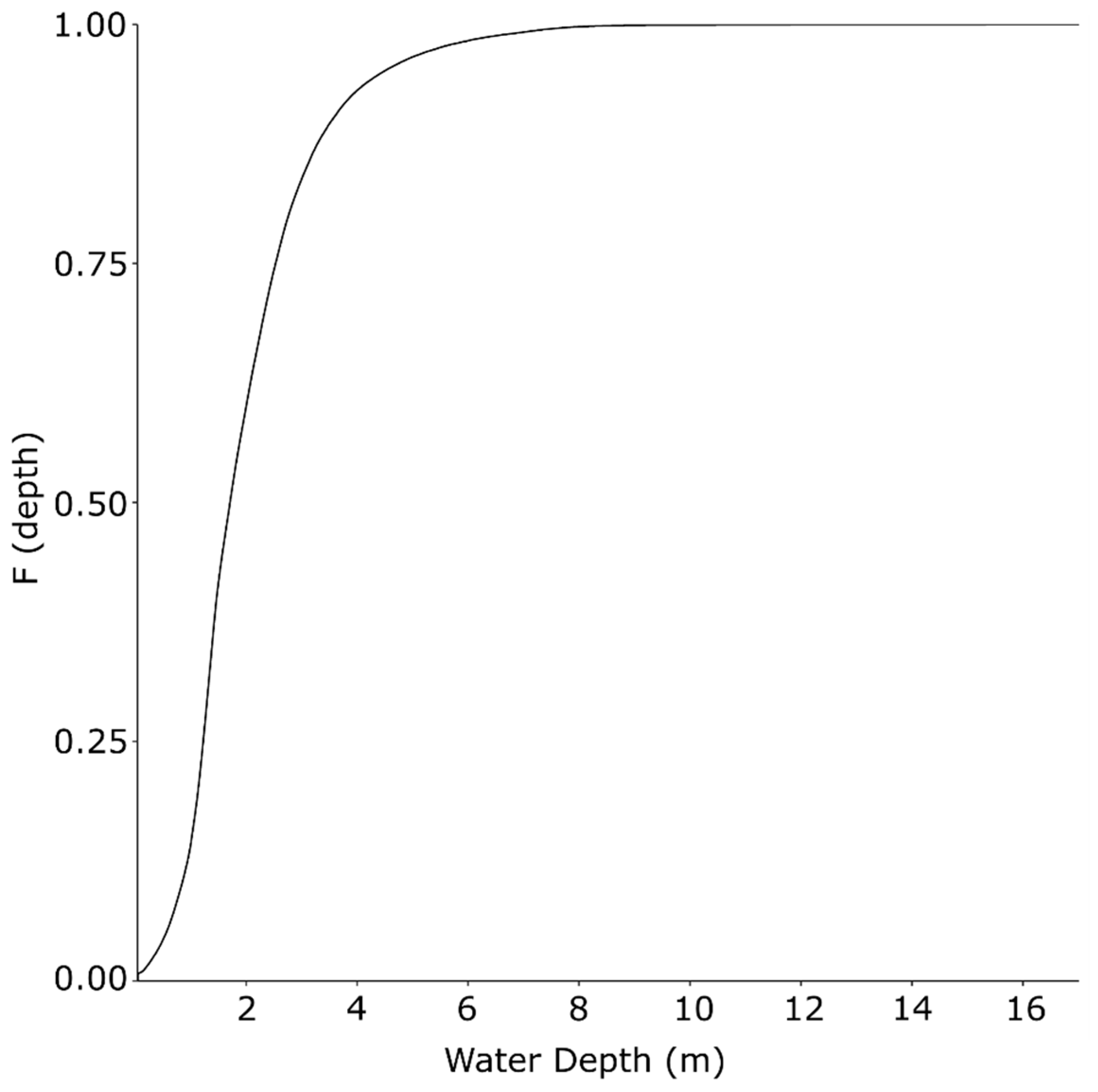
The study area was located between the Mactaquac Generating Station (MGS, 45.955492, −66.866947) and the City of Fredericton (45.968891, −66.644873), where the river‘s average width is 750 m [45] and the depth during typical summer flow conditions (425 m³s⁻¹) is mainly shallower than 8 m (Figure 1, [46]). The mean monthly discharge at MGS varies between 202 m³s⁻¹ and 2280 m³s⁻¹ (1995–1999 data, Government of Canada, Water office (http://wateroffice.ec.gc.ca/), downloaded 1 March 2016). The average water clarity, measured as Secchi depth, is between 0.4 m and 1.8 m in the summer [47].

2.2. Field Procedures

The data were collected from June to August 2015 when the water temperature varied between 17 °C and 28 °C. Data of depth, bottom hardness, and presence/absence of vegetation were collected along 25 m transects. The transect was marked with a floating rope that was placed in the river using anchors and buoys at both ends. The rope was marked every 5 m (0 m, 5 m, 10 m, 15 m, 20 m, 25 m). Buoys and anchors were set at a 3-m distance from the start (0 m) and end (25 m) of the transect to reduce interference. In order to ensure that a representative variety of depths and bottom substrate types available in the studied reach were assessed, transect locations were chosen haphazardly by the field crew. The field crew was tasked to target as many different types and combinations of habitat as they could find in the study area. The majority of the transects were oriented from upstream to downstream to minimize the impact of the flow. Where flow conditions allowed, some transects were measured perpendicular to the flow.

Lowrance HDS 5 (Gen 2) and HDS 7 (Gen 2) fish finders with 83/200 kHz skimmer transducer (22° beam width), collectively the hydroacoustic device, were used to capture bathymetric and physical habitat data. The device records the GPS position typically every second and averages the acoustic data between GPS positional reports (5 to 30 pings) for each coordinate point [48]. Settings in Lowrance units during all sampling events were: Fishing Mode = Shallow Water, Ping Rate = 15, Range = Auto, Frequency = 200 kHz, and WAAS = Enabled [48]. The pulse length in the Lowrance unit is dynamic and automatically optimized to depth range [48].

Hydroacoustic data were recorded using two approaches:

• The transducer was held over each measuring point for 1 min of recording at 10 cm depth from surface (fixed point: non-mobile), and
• The transducer was mounted at the transom of the boat to 15 cm depth from surface and the boat was driven over the entire transect (whole transect point: mobile).

Suggested speeds for EcoSound mapping range from 1.6 to 11.3 km/h [48]. Speeds between 5.6 and 9.5 km/h were used in this study. Variation in speeds at different transects was unavoidable due to different flow conditions. Boat speed was measured using the hydroacoustic device.

A single transect was surveyed in a very shallow area (<0.8 m) where the boat was pulled manually by a person at a speed 1.3 km/h. The data from that transect was analyzed separately to assess EcoSound depth accuracy for areas where the depth was below the EcoSound depth-limit (0.37 m) [48].

For comparison to hydroacoustic data, manually obtained physical measurements were collected every 5 m for a total of six points along every transect. These measurements were used to validate the data provided by the hydroacoustic device. The validation data for water depth was obtained by using a pole (shallow areas) or a rope attached to a closed Ponar sampler. Substrate was assessed by using a Ponar grab sampler. Substrate size was visually estimated using a modified Wentworth scale ([47],

Table 1. Substrate grain sizes found in the study area classified using modified Wentworth scale. Substrate classes that were identified at the studied reach are indicated in bold font.

Class	Size	Name
1	n/a	Fine organic
2	n/a	Coarse organic
3	<0.1 mm	Silt/Clay
4	0.1 mm–2 mm	Sand
5	2 mm–2 cm	Gravel
6	2–3 cm	Small pebble
7	3–6 cm	Pebble
8	6–12 cm	Small cobble
9	12–25 cm	Cobble
10	25–38 cm	Large cobble
11	38–52 cm	Boulder
12	>52 cm	Large boulder
13	n/a	Bedrock

). Aquatic vegetation was visually assessed and recorded as present or absent at each of the six sampled points. In deeper areas where visual confirmation of macrophyte presence was not possible, a macrophyte rake (35 × 12 cm with 2 cm spacing) was thrown three times, and if macrophytes were retrieved in any replicate, it was used as a positive confirmation of their presence at the sampled location.

A separate dataset was collected for vegetation biovolume (height in % of water column) assessment. Vegetation height was recorded by manual observation (snorkeling) using 5 categories of percent vegetation in relation to the height of the water column (0%, 1–25%, 26–50%, 51–75%, 76–100%). The vegetation height was recorded manually in 0.5 m intervals along a 25 m transect. The same transects were assessed for vegetation height using hydroacoustics: The transects were driven using speeds between 4 and 6.4 km/h, and the location of the start and end point of the transect was recorded using the internal GPS of the hydroacoustic device. Vegetation biovolume in the study area was highly variable and the predominant macrophyte species in the Saint John River were found to be Myriophyllum spp., Potamogeton spp., and Vallisneria spp. The majority of transects measured for biovolume were from areas dominated by aquatic grass (Vallisneria spp.).

2.3. BioBase Ecosound

EcoSound is a cloud-based automated data processing tool that facilitates rapid creation of aquatic habitat maps from data collected using low-cost consumer hydroacoustic devices. The hydroacoustic device must be capable of recording a 200 kHz signal with internal GPS to a .sl2 file (Lowrance, Simrad, or BMG) [48]. The uploaded data is processed through EcoSound programs and the data is subjected to quality control analyses [48]. Data failing quality assurance tests are removed from the data considered for summarization: EcoSound minimum depth for vegetation and bottom hardness detection is 2.4 ft. (0.73 m) from the transducer face and 1.2 ft. (0.37 m) for depth. Bottom hardness is not recorded where vegetation fills >60% of the water column [48]. Maximum speed for mapping with EcoSound is 32 km/h (20 mph) for depth, 19 km/h (12 mph) for vegetation, and 16 km/h (10 mph) for bottom hardness [48].

Following data validation, feature-detection algorithms were used and the resulting data were processed through ordinary point kriging algorithms in EcoSound [48]. These algorithms predict values in unsampled locations based on the geostatistical relationship of the input points. [35,48]. As an output, EcoSound creates GIS layers of depth, vegetation biovolume (macrophyte height in % of water column) and bottom hardness [48]. Bottom hardness is estimated from the acoustic reflectivity of the bottom second echo (E2) (Ray Valley/BioBase EcoSound, personal communication) and the values are on a relative but continuous scale that ranges from 0–0.25 (soft), 0.25–0.4 (medium) to 0.4–0.5 (hard) [48]. The distance between the river bottom and the top of the plant canopy (tallest plant intercepting the acoustic cone) was recorded as the plant height for each ping [48]. Plant heights were averaged across all pings within a GPS coordinate point, and plant heights that together averaged less than 5% of the depth were considered not vegetated to minimize false detections by bottom detritus or other debris. EcoSound also discards 2% of the deepest coordinate points registering vegetation to prevent bottom debris or other phenomena from generation of false vegetation detections [48].

The point data at transect GPS locations was downloaded from EcoSound and used in this study without predicted values in unsampled locations, in order to test the accuracy of the actual hydroacoustic measurements at sampling locations.

2.4. Data Processing and Statistical Analysis

The fixed point data were exported from EcoSound as x, y, z point tables and transducer depth was added to the EcoSound depth and vegetation values. The variation of the recordings at each fixed point was examined and if the depth data points were found to be erroneous (i.e., clearly different compared to the rest of the data) at the beginning or at the end of the one minute measuring period, they were removed because the difference was assumed to be due to handling of the equipment (e.g., moving of the transducer). Normality of the fixed point data was tested with Shapiro-Wilk test using SPSS statistics 22 software. The following values were calculated for each fixed point from the one-minute period and included in the analyses: mean (depth), median (bottom hardness, vegetation), minimum (vegetation), and maximum (vegetation). Maximum and minimum vegetation height were used to find the differences during the one-minute measuring period for vegetation presence/absence data: if the maximum value was zero, all the measurements during the one-minute period showed vegetation absence at that fixed-point location.

The whole transect data were also exported from EcoSound as x, y and z point tables and transducer depth was added to the EcoSound depth and vegetation height values. The locations of the fixed point measurements were used to identify the same locations from the whole transects in Qgis 2.8.2-Wien Software. The whole transect data were then extracted to point data of depth, vegetation and bottom hardness, of these same locations. The data were extracted manually from the locations where the transect points were clearly near the fixed point location. If there was no data at the location, it was saved as a “no data” point. If there were multiple recordings at a single location, a maximum of five points were chosen randomly and their mean was used in analysis for depth, bottom hardness and vegetation.

For macrophyte transects, the linear distance from start point was calculated for each EcoSound data-point on the vegetation biovolume transects using a Distance Matrix tool in GIS-software (Qgis 2.8.2-Wien). If the distance between the GPS recorded start and end point was calculated to be more than 26 m, the transects were not used in the analyses due to GPS inaccuracy, as the exact location of the measurement would not have been known. Using the manual observation data, locations where the macrophyte bed was uniform (no change in macrophyte height) within 2 m distance were selected for the analysis. This selection was done to minimize the effect of spatial autocorrelation (i.e., difference in biovolume during one hydroacoustic recoding period). The data were classified into their respective manually assessed biovolume categories and the hydroacoustic measurements of the biovolume were compared to manual observations at the same distance from the start point. The vegetation transects were also analysed as whole 25 m transects, where all manually observed and hydroacoustically recorded points between the start and end location were saved.

2.5. Depth

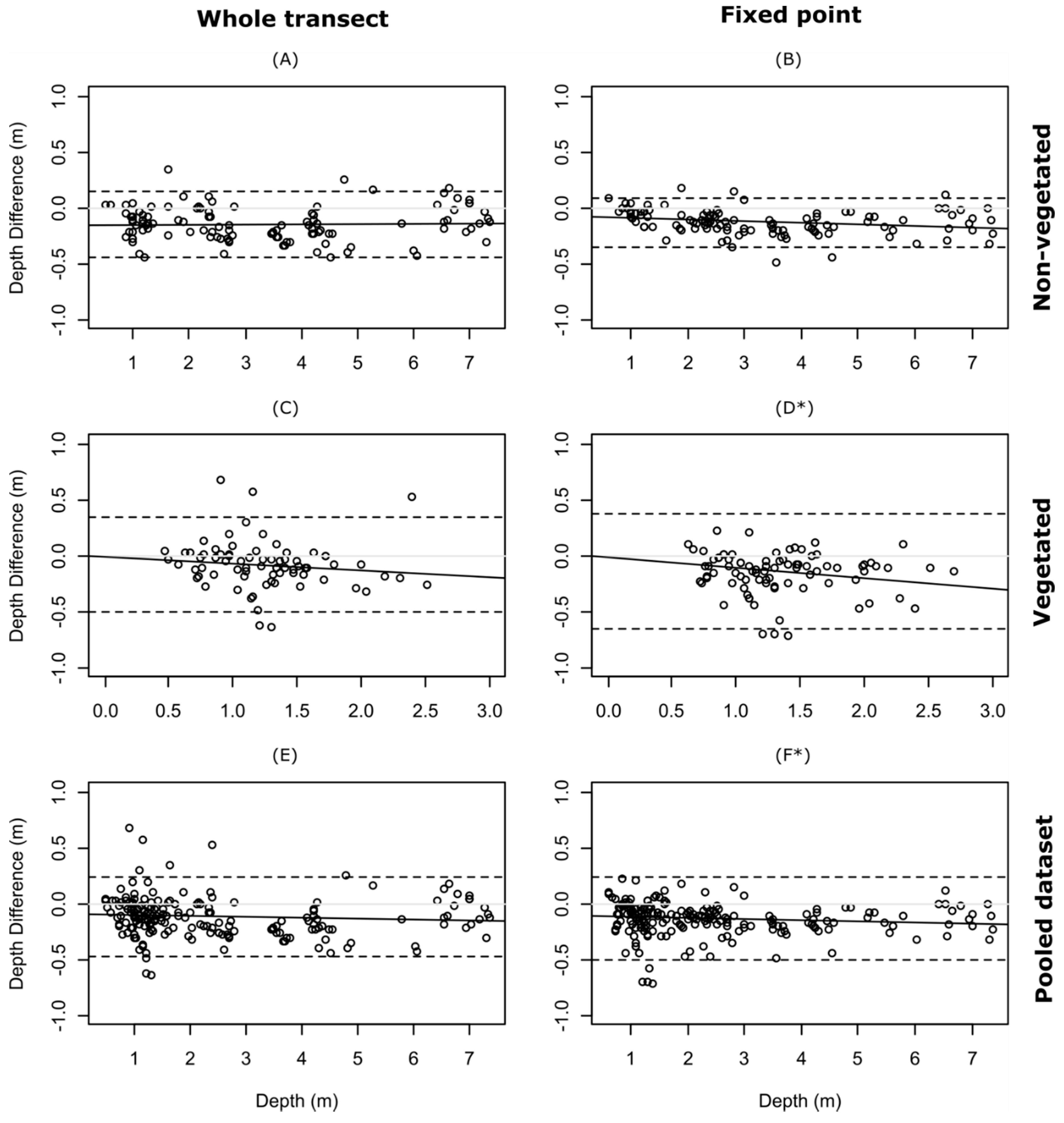
The depth data were analysed for non-vegetated areas and vegetated areas separately, but also for the pooled dataset. Mean absolute error (MAE) and standard deviation were calculated from the absolute difference between depth rod/rope measurements and EcoSound depth values. Bland–Altman method [49] was used for comparing the depth measurements to the manual measurements that were used as a standard: Bland–Altman bias was defined as the mean difference between depth rod/rope measurements and EcoSound depth values, and the limits of agreement were calculated as bias ± 1.96 SD of difference, defining the range within which 95% of the differences of the hydroacoustic method fall in comparison to rod/rope measurements. Ordinary least-squares regression was used in the plot to detect possible proportional differences and one-sample test of the major axis slope was used in R (R core team version 3.0.2) to test if the slope of the regression line differed significantly from 0. The statistical difference between the overall mean of differences and zero was tested (one-sample t-test) using R software (R Core Team version 3.0.2).

On the single transect that was measured at the very shallow area, MAE and standard deviation were calculated to assess EcoSound measurements below and above EcoSound depth detection limit.

2.6. Bottom Hardness

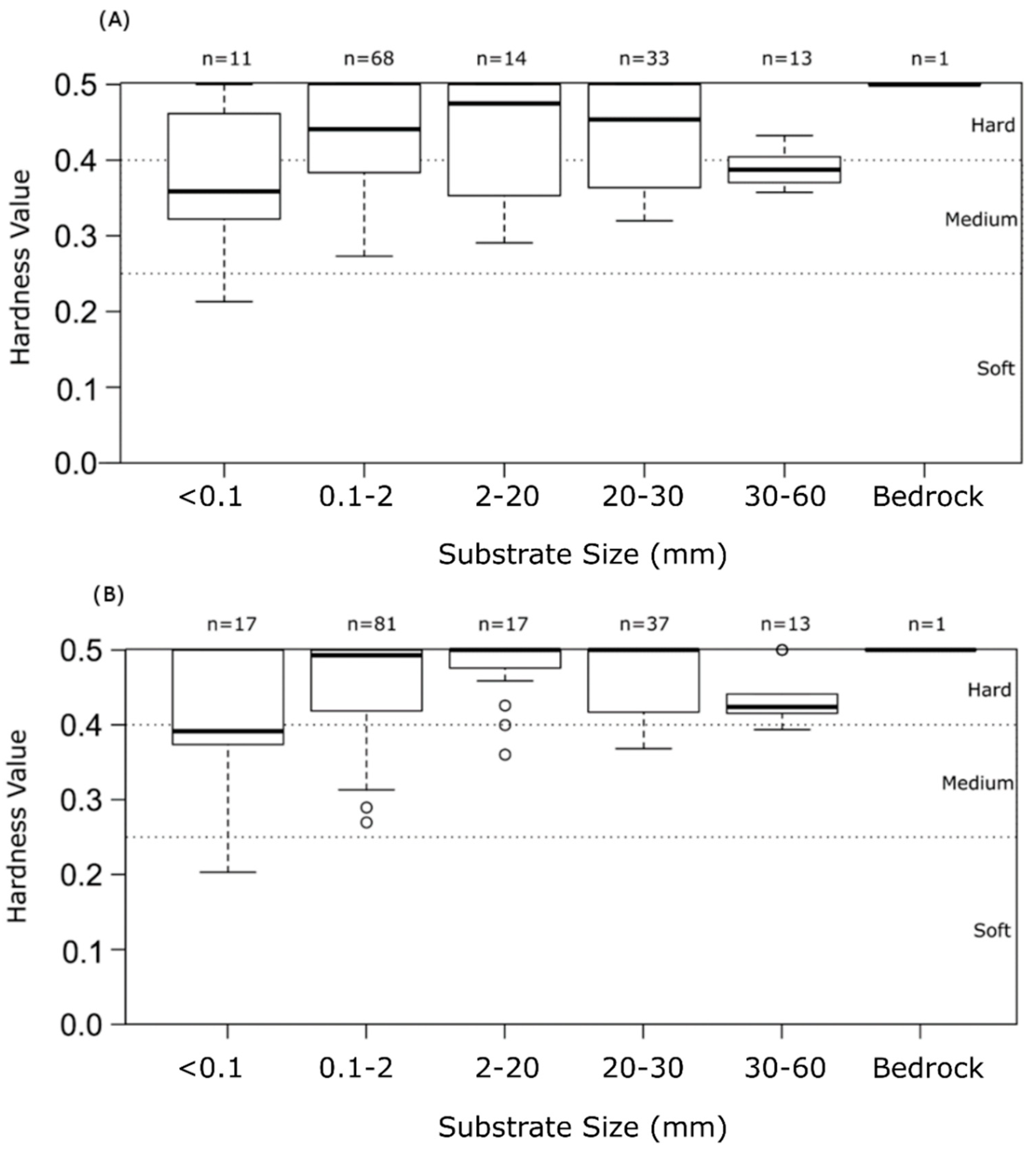
Normality of the EcoSound hardness values in each substrate size category was tested using the Shapiro-Wilk test and the median of the EcoSound hardness values was calculated for each substrate size category. The nonparametric Kruskal–Wallis test was used to determine if hardness values significantly varied between the different bottom types of manual observation categories. When significant differences were found, pairwise tests (Mann–Whitney U-test, SPSS statistics 22 software) were conducted.

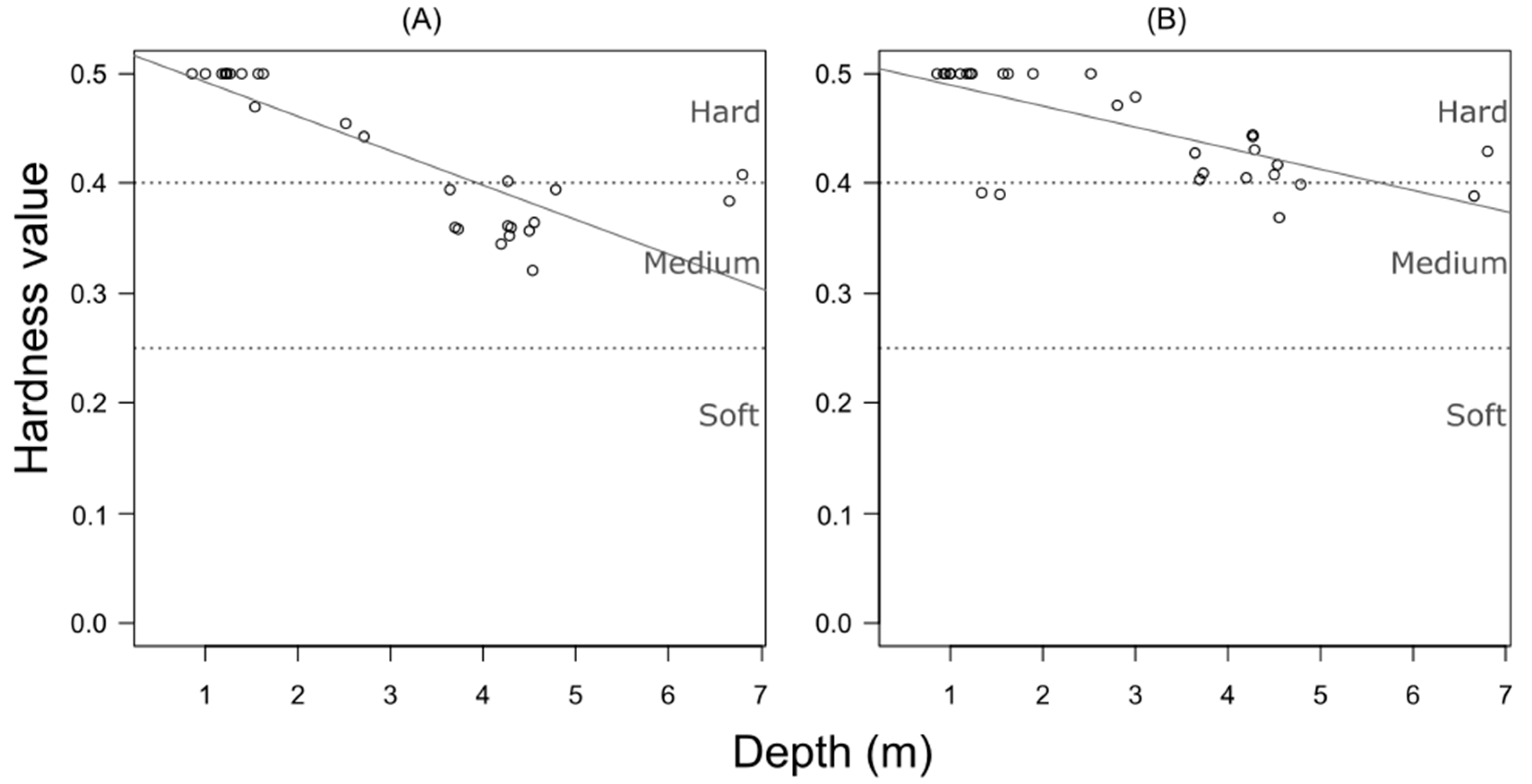
The impact of depth on hardness interpretation in the EcoSound data was examined using the data from a fixed substrate size class 6 (2–3 cm, small pebble). Class 6 was chosen for comparison because it was a substrate size class that was found throughout the whole studied depth range. Normality of the data was tested with a Shapiro–Wilk test using SPSS statistics 22 software and Spearman’s correlation test was used using R software (R Core Team version 3.0.2).

2.7. Vegetation

Vegetation fixed point data were divided into non-vegetated (0% biovolume) and vegetated (>0% biovolume) areas and compared to field observations of vegetation presence.

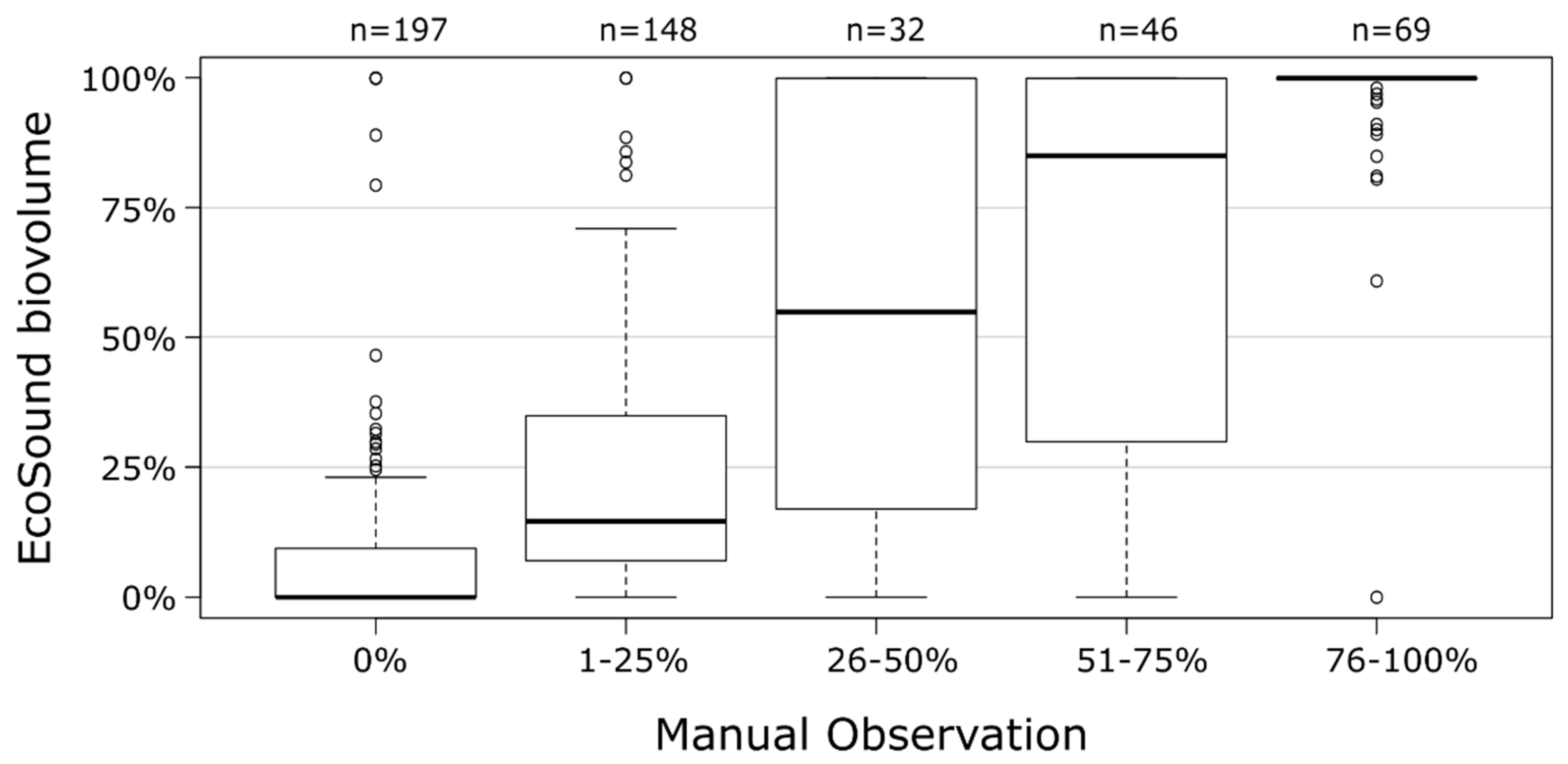
The vegetation biovolume data were grouped into the five categories used for manually assessing the vegetation height. The normality of biovolume values in the categories were tested using the Shapiro–Wilk test, and the median was calculated for each category. The differences between vegetation biovolume values of observation categories were tested using the nonparametric Kruskal–Wallis test. When significant differences were found pairwise tests (Mann–Whitney U-test) were conducted. Tests were run using SPSS statistics 22 software. The EcoSound values were grouped using the same categories, and the agreement between the two methods was assessed using Cohen’s weighted (squared) Kappa in R software (R core Team version 3.6.0) using ‘irr’ package.

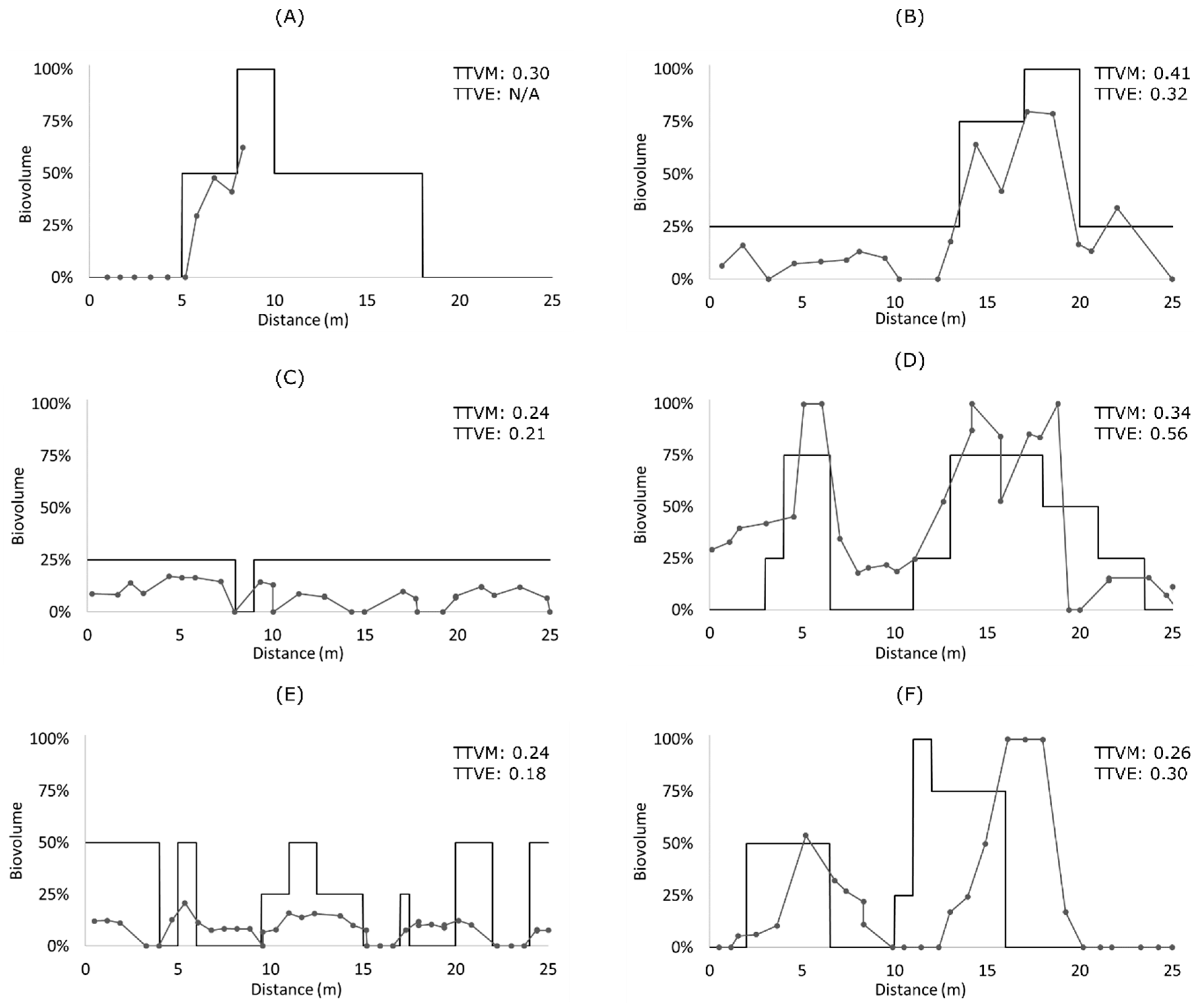
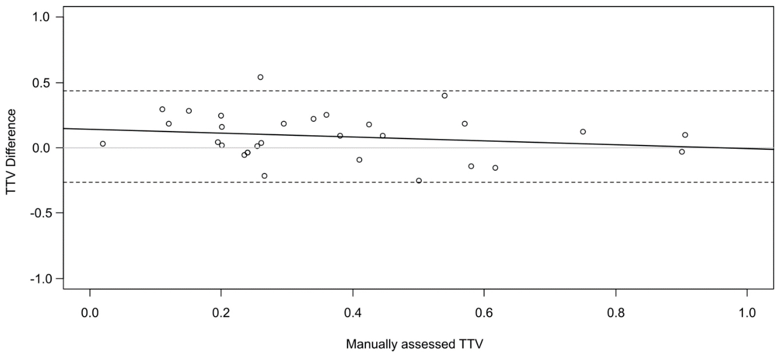
Manually and hydroacoustically assessed biovolume values were also compared using the whole 25 m transects. The upper limit of each category was used for all manually assessed data points (i.e., 25% was used for 1–25% category), and the transects were plotted as X–Y (biovolume-distance) graphs. The EcoSound biovolume values were then classified to their respective categories, using the same five vegetation height categories as for manually assessed data, and the upper limit of each category was used for calculating a total transect vegetation (TTV) value for both methods for each transect by multiplying the biovolume value at each point by distance to the next measurement, and dividing it by the total length of the transect. The TTV value represents the amount of vegetation in each transect, with 1 being a transect where the whole 25 m transect has vegetation up to the surface (100% canopy height), and 0 is a transect with no vegetation. The TTV values of the two methods were compared using Bland–Altman difference plot method [49] and ordinary least-squares regression was used in the plot to detect possible proportional differences. A one-sample test of the major axis slope was used in R (R core team version 3.6.0) to test if the slope of the regression line differed significantly from 0 and the statistical difference between the overall mean of differences and zero was tested (one-sample t-test) using R software (R Core Team version 3.6.0). Transects that had >5 m gaps between any nearest EcoSound measurements (e.g., due to very dense vegetation) were not used in this analysis.

3. Results

3.1. Depth

The mean absolute error between the manual depth measurements and EcoSound depths was 0.17 ± 0.13 (average ± 1SD) m for transect data and 0.17 ± 0.16 for fixed point data (

Table 2. Mean absolute error (MAE) with 1 SD, Bias, and 95% limits of agreement (LOA) of depth measurements for areas with and without vegetation, and for the pooled data.

	No Vegetation					Vegetation					Pooled Data
	n	MAE	Bias	LOA		n	MAE	Bias	LOA		n	MAE	Bias	LOA
Whole transect	113	0.18 ± 0.11	−0.15	−0.44	0.15	74	0.17 ± 0.16	−0.09	−0.51	0.34	187	0.17 ± 0.13	−0.12	−0.48	0.24
Fixed point	111	0.14 ± 0.09	−0.13	−0.35	0.09	86	0.20 ± 0.22	−0.14	−0.65	0.38	197	0.17 ± 0.16	−0.13	−0.51	0.24

). The mean differences deviated significantly from zero on all the datasets (1-sample t-test, p < 0.05, Figure 2).

The relative Bland–Altman bias for whole transect measurements was −0.15 m and −0.09 m at non-vegetated and vegetated areas, respectively, and −0.12 m for the pooled data (Figure 2A,C,E; Table 2). The difference between the limits of agreement was larger (from −0.51 to 0.34) at vegetated areas than at non-vegetated areas (from −0.45 to 0.15). There was no trend in bias between the two methods relative to the manually measured depth on vegetated (p = 0.29), non-vegetated (p = 0.76), or for the pooled dataset (p = 0.24) (Figure 2A,C,E).

The relative Bland–Altman bias for fixed point measurements was −0.13 m and −0.14 m at non-vegetated and vegetated areas, respectively, and −0.13 m for the pooled data (Figure 2B,D,F; Table 2). Similarly to the whole transect data, the difference between the limits of agreement was larger (from −0.65 to 0.38) at vegetated areas than at non-vegetated areas (from −0.35 to 0.09). There was no trend in bias between the two methods relative to the manually measured depth on vegetated (p = 0.12), non-vegetated (p = 0.09), or for the pooled dataset (p = 0.16) (Figure 2B,D,F).

On the transect that was measured on the very shallow (<0.7 m) non-vegetated area, four of the six locations were under the EcoSound dept-limit (1.2 ft/0.366 m). Three of the four fixed point and four whole transect measurements passed the EcoSound programs and were reported for the user: the depths were overestimated at all the locations and the MAE was 0.49 ± 0.24 m for whole transect and 0.30 ± 0.05 m for fixed point measurements. At the two locations that were above the detection limit, the MAE was 0.19 ± 0.20 m for whole transect and 0.03 ± 0.01 m for fixed point measurements.

3.2. Bottom Hardness

For all the observations, 79% of the fixed point and 63% of the whole transect measurements were in the ‘hard’ category (hardness > 0.4) and the only ‘soft’ values (hardness < 0.25, 2 fixed point locations and 1 whole transect) were registered in the class 3 substrate type (<0.1 mm silt/clay). When grouped into different hardness categories based on manual measurements, the median of the measurements was hard in all the categories except classes 3 (<0.1 mm silt/clay) (whole transect data, Figure 3A: fixed point data, Figure 3B) and 7 (3–6 cm pebble) (whole transect, Figure 3B). The variation of EcoSound hardness values was higher on smaller substrate type classes (Figure 3).

Significant differences between the hardness values of the substrate size classes were found among the fixed point measurements ($x^2\left(2\right)=14.5, p<0.05$, Figure 3B), but not among whole transect substrate estimates ($x^2\left(2\right)=10.2, p=0.07$ Figure 3A). A pairwise test with Bonferroni correction for the fixed point measurements showed a significant difference only between groups 3 (<0.1 mm silt/clay) and 7 (30–60 mm pebble) (p < 0.05).

There was a significant negative correlation between the EcoSound Hardness value and depth when measured on the fixed substrate class 6 (20–30 mm; small pebble), for the both fixed point (Spearman’s correlation, $\mathsf{\rho }\left(28\right)=-0.73, p<0.05)$ and the whole transect measurements ($\mathsf{\rho }\left(25\right)=-0.78, p<0.05$) (Figure 4).

3.3. Vegetation Presence/Absence

EcoSound registered vegetation at 85% of vegetated whole transect measurement points and at 94% of vegetated fixed-point locations (

Table 3. Accuracy of EcoSound for registering manually assessed vegetation presence/absence on whole transect and fixed point (median of one-minute period) measurements.

	Moving Boat			Fixed Point
	n	Vegetation Registered	No Vegetation Registered	n	Vegetation Registered	No Vegetation Registered
Vegetation	47	85%	15%	64	94%	6%
No Vegetation	105	10%	90%	111	0%	100%

).

No vegetation was registered at 90% of non-vegetated whole transect measuring points and at 100% of non-vegetated fixed points (median of one-minute measuring period, Table 3). Some vegetation, however, was recorded during the one-minute fixed point recording period (maximum value of the period was >0%) at 17 non-vegetated spots, of which 6 were located in high velocity areas.

3.4. Vegetation Biovolume

Of all 492 biovolume measurements, EcoSound values differed from manual observations in 219 (45%) instances. The EcoSound value was higher than what was manually observed in 163 (74%) of those instances. Weighted Kappa (0.73) indicated good agreement between the two methods.

When grouped into the five different manual observation categories, a significant difference between the EcoSound biovolume values (percent vegetation in relation to height of water column) was found with the Kruskal–Wallis test ($x^2\left(2\right)=247.9$, p < 0.05) (Figure 5). A post-hoc Mann–Whitney test with Bonferroni correction showed significant differences between all the groups (p < 0.05) with the exception of no significant difference between 26–50% and 51–75% (p = 1.0) or 26–50% and 76–100% (p = 0.095).

The median of the EcoSound biovolume was in the same category as manual observation at categories 0%, 1–25%, and 76–100% (Figure 5). EcoSound reported 100% biovolume at multiple locations at categories 26–50% (44% of locations) and 51–75% (59% of locations), and, as a result, the median was in a higher category than manually reported (Figure 5).

The X–Y plots (n = 30) reveal that the two methods assessed the patterns of change in vegetation height similarly, although the absolute values were often different and EcoSound showed changes in biovolume with a smoother pattern than what was observed during the manual observation measurements (Figure 6). Three vegetation biovolume transects were removed from this analysis because not enough datapoints were reported by EcoSound: a densely vegetated area was reported in all of those transects (Figure 6A). The methods were most similar on transects where the changes in biovolume were clear and small, or the biovolume stayed constant throughout the whole transect (Figure 6B,C). The Ecosound total biovolume was higher at 70% of the transects (Figure 6D), and the manual measurements were higher at 30% the transects (Figure 6E). The changes in biovolume between the two methods appeared at clearly different distance from starting point at approximately 7% of the transects, indicating a lag in EcoSound recording of data (Figure 6F).

The mean value of differences between manually and Ecosound-assessed vegetation as a TTV value deviated significantly from zero (1-sample t-test, p < 0.05) with the relative Bland–Altman bias of 0.09 and the limits of agreement between −0.26 and 0.44 (Figure 7). However, there was no trend in bias between the two methods relative to the absolute TTV value on transect (p = 0.33).

4. Discussion

4.1. Depth

The EcoSound depth values were on average 9–15 cm shallower than the rope/rod measurements across the assessed depth range. The error in depth measurement was greater in areas with vegetated river bed than on non-vegetated river bed. There was no significant trend in bias between the two methods relative to manually measured depths, hence the error is constant throughout the measured depths (Bland–Altman fixed bias). Therefore, the relative error was smaller in deeper versus shallower depths. In general, measuring depth with the hydroacoustic method in areas deeper than the EcoSound limit of 1.2 ft. (0.37 m) can be considered reliable and the bias defined in this study can be used to correct future mapping measurements in similar study environments.

The hydroacoustic measurement overestimated the depth in areas where the distance between transducer and the river bed was less than the EcoSound limit < 1.2 ft. (0.37 m). The overestimation in these locations resulted the data passing the tests in EcoSound programs and being falsely reported for the user. Using the hydroacoustic/EcoSound combination for mapping in these shallow areas should therefore be avoided, but is also limited in practice when using a motorized boat equipped with propeller-propulsion outboard motors.

The depth error of EcoSound has not been reported before, but a previous study tested Biosonics DT4000 transducer with SAVEWS (currently marketed under the trade name EcoSAV) software and reported a 2.5 cm depth overestimation using a sample of 12 points in vegetated areas [33]. However, their smaller dataset and different data analysis render the comparison between SAVEWS [33] and EcoSound [this study] challenging.

4.2. Bottom Hardness

EcoSound hardness values were very similar at all the measured areas irrespective of the manually measured substrate class, and no significant differences were found between the six substrate size classes which ranged from clay/silt to bedrock. The resulting river bottom hardness values exhibited little variance and the value was high (hard category: 0.4–0.5) at most of the measuring points. Previous studies conducted in lakes have shown a wider range of EcoSound hardness values and the output has been successfully used to determine different bottom types [36,39,40]. The softest values were recorded on “muck”, mud, and silt [39,40], which were mostly missing on our study area. Most of the silt/clay bottoms in our study area were located in the near-shore areas where depth was preventive of the use of the EcoSound method, and therefore the amount of data collected was lower in that substrate size class. The only “soft” hardness values were recorded on silt/clay bottoms, which indicates that when softer values are recorded, the substrate size is indeed smaller. Although we only tested the substrate hardness in different substrate size classes, there are other factors that can influence bottom hardness than just substrate size. Testing of other attributes, such as water content and bulk density would be examples of making the bottom hardness value measurement more representative. This can especially be the case in smaller substrate classes where the variation of the hardness values was higher.

Small changes in hardness values, when observations are stemming from different depths, should be interpreted with caution. In this study, although we only tested on one substrate size (for standardization purpose), lower hardness values were registered at deeper areas than at shallower areas for similar bottom types. Similar reports of potential depth biasing have been reported using the Biosonics VBT Seabed Classification Software [50].

Other approaches for acoustic signal processing may be more informative for substrate size separation in a large river environment such as that we studied. For example, significant correlations between echo features and mean grain size have been found [51] and the acoustic properties of lake bottom sediments have been shown to correlate with a number of physical and chemical properties, including textural information, water content, and organic carbon and total nitrogen contents [52]. There are other software that report bottom roughness with substrate hardness values [53], even from the same .sl2 files recorded with Lowrance (e.g., Reefmaster Software Ltd., Birdham, United Kingdom) and they may reliably differentiate between substrate types. Confirming the functionality of these methods for substrate classification warrants future studies.

4.3. Vegetation

The results show that EcoSound registers vegetation presence/absence very well. Vegetation, when present based on manual surveys, was registered using EcoSound at 94% (fixed point) and 85% (whole transect) of the locations. Vegetation was registered also at locations where only one plant was under the transducer and where the plants were growing further upstream, but the flow pushed the canopy below the transducer. Vegetation was falsely registered on non-vegetated bottoms at 0% (fixed point) and 10% (whole transect) of locations, some of which were found in high velocity areas where background noise might have been mistaken for plant detections.

EcoSound registered macrophyte height (biovolume) reasonably similarly to manual observations: EcoSound assessed vegetation height in the same vegetation category as manually observed 55% of the measurements, and the weighted Kappa value indicated good agreement between the two methods. EcoSound assessed vegetation height most accurately at categories 0%, 1–25%, and 100%. EcoSound was less accurate at categories 26–50% and 51–75%, where the variation of the EcoSound biovolume values was higher, and EcoSound reported 100% biovolume for many locations. The results were similar when the data were analyzed over the whole 25 m transects, as there was a generally good agreement between the hydroacoustic and manual method, although the EcoSound estimate was typically higher. EcoSound showed changes in biovolume with a smoother pattern than our manual observations, which was a result of the categorial style of recording the manual observations: the Hydroacoustic method can sample and produce a higher resolution with regard to information about vegetation height, and much faster than manual observations.

Previous studies have also reported a positive correlation between manually observed biovolume and the Lowrance/EcoSound system [35,38], and, similarly to this study, the Lowrance/EcoSound system has produced higher estimates when compared to plant community observations [28].

EcoSound reports the vegetation height for any part of a plant that reflects an acoustic signal and therefore river flow will have a small-scale impact for mapping as the canopies are pushed over by the flow. Transducer depth may also confound measurements of aquatic vegetation. For instance, if the aquatic plant is in close proximity to the transducer field where the acoustic beam is not properly formed (transducer near field), its actual location in the acoustic cone may be unknown [23].

Because EcoSound reports the average of measurements between GPS locations, it results in smoother changes in macrophyte height compared to manual observations, which can cause a source of error on patchy macrophyte beds. The accuracy can be increased by using slower boat speeds, as the fixed point measurement generally had higher accuracy compared to when the boat was moving.

At 7% of transects, changes in EcoSound biovolume appeared at different distances from the start point compared to manual observations. It is possible that this was caused by GPS location error during hydroacoustic recording, however, a small spatial shift (i.e., <1 m) in the true location of a macrophyte bed is likely insignificant for most real-life applications where the interest is to produce maps of aquatic vegetation volume.

4.4. Error Sources

Flowing water, wind, and waves can all cause errors for manual measuring processes but also for the hydroacoustic signal because transducer depth and its attack angle (in which it faces the bottom) is affected. The impact of the GPS error was minimized in this study by the use of physical ropes as transects, but it causes small uncertainties because the starting and end points of the whole transects were marked using GPS location. It is also possible that the GPS location changed during the whole transect surveys and caused small positional errors. In addition, Lowrance skimmer transducer samples a different cross-sectional area than the Ponar-sampler used for manual observations, and the difference increases as a function of increasing depth. For example, the Ponar-sample used in this study always samples 0.02 m² rectangular area, while the transducer with 22° beam width samples a theoretic circle of 0.03 m² at 1 m depth and 1.9 m² at 8 m depth. Steep slopes present a challenge for bottom typing because the acoustic beam is intercepted at an angle, and typically, a soft bottom will be reported when recording data parallel to a steep slope [48]. It can also be problematic for defining the exact location of manual sampling. The river bottom is assumed to be uniform in fine lateral scale, and therefore, said errors are thought to cause only minor differences in the results. However, when mapping over a steep slope, a perpendicular recording path is recommended [48].

The accuracy of a produced map is also controlled by the spatial coverage of the measurements in the study area (i.e., transect spacing and boat speed) [54], interpolation method [54], and GPS error. The user can control the coverage by varying boat speeds and transect spacing and, if needed, external GPS units can be used to increase the GPS accuracy of fish finders. The interpolation method was not tested in this study, but three methods were tested for mapping an aquatic environment in a similar setup [54]. EcoSound uses a kriging algorithm that is not controllable by the user when using basic EcoSound settings, but more advanced users can download the point data and use their own interpolation method in GIS software. However, the readily interpolated mapping is a product that may add significantly to the usability of this application, particularly to many NGO user-groups who do not have ready access, or the skillset, to programs capable of spatial interpolation.

5. Conclusions

In this study, the accuracy and precision of the hydroacoustic measurements of physical and biological characteristics were described. Our results, in conjunction with previously published studies, support the notion that accuracy of a low-cost hydroacoustic system comprised of Lowrance/EcoSound fish finder measurements for depth and vegetation presence/absence is generally reliable for habitat mapping in large rivers. EcoSound assigned vegetation height (EcoSound biovolume) correctly in 55% of instances, but often overestimated it in other instances. It was most accurate when the vegetation canopy was ≤25% or >75% of the water column. The current version of EcoSound did not differentiate bottom type in rivers composed largely of hard substrates even though the existing bottom hardness algorithm in the EcoSound software is useful for softer substratum habitats such as lakes and seabeds.

Since the needed spatial resolution of river maps is often low, the effect of errors described in this study is negligible. If the targeted area is very shallow in depth and below the detection limits of EcoSound, other methods should be considered, or alternatively, mapping of the shallow areas may be conducted during the flood season when more water between the targeted feature and the transducer is available.

Hydroacoustic data collection and analysis using the combination of Lowrance HDS and EcoSound is fast and hardware, as well as analysis, costs are substantially lower than with many other acoustic methods [28,36]. Low-cost methods for mapping can benefit researchers and resource managers when the highest accuracy and resolution is not needed.