Conservation Biogeography of Tenebrionid Beetles: Insights from Italian Reserves


Department of Life, Health and Environmental Sciences, University of L’Aquila, Via Vetoio, 67100 L’Aquila, Italy
Diversity 2020, 12(9), 348; https://doi.org/10.3390/d12090348
Submission received: 23 August 2020
/
Revised: 5 September 2020
/
Accepted: 7 September 2020
/
Published: 10 September 2020
(This article belongs to the Section Biogeography and Macroecology)
Abstract
:The species-area relationship (SAR), the latitudinal gradient, the peninsula effect, and the elevational gradient are widespread biogeographical patterns. Using data from Italian reserves, these patterns were tested for tenebrionids and used as a framework to calculate expected extinction rates following area loss. Area was an important determinant of overall tenebrionid species richness, but not for xylophilous and endemic species. Thus, focusing on reserve areas is not the best approach for conserving insects with specialised ecology and restricted distribution. In general, species richness declined northwards, which contrasts with the peninsula effect, but conforms to the European latitudinal pattern observed in most taxa because of current and past biogeographical factors. Minimum elevation had an overall negative influence, as most tenebrionids are thermophilic. However, xylophilous tenebrionids, which are mainly associated with mesophilic forests, did not decline northwards, and were positively influenced by higher elevational ranges that allow more forms of vegetation. SAR-based extinction rates reflect species dispersal capabilities, being highest for geophilous species (which are mainly flightless), and lower for the xylophilous species. Extinction rates based on multiple models indicate that the use of area alone may overestimate extinction rates, when other factors exert an important role in determining species richness.
1. Introduction
Italy is located in the centre of the Mediterranean basin, one of the world’s biodiversity hotspots [1,2,3]. Italy shows an extraordinary diversity of species for the most disparate plant and animal groups [4,5], as a consequence of both current factors, such as the variety of climatic conditions and landscapes [6], and the past history of its territory, in particular its role as a crucial refuge and evolutionary centre during Pleistocene glaciations [7,8,9,10].
Italy hosts some 900 protected areas [11], and another 400 areas that benefit from some form of protection [6], accounting for a total surface area of about 3.5 million hectares (more than 11% of Italian land). For most areas, however, faunal knowledge is still very poor, especially for invertebrates, which, of course, represents a serious limit to effective conservation actions.
Among the few invertebrates for which there is information about the number of species present in some reserves, beetles play a prominent role, with relatively abundant data on their distribution, at least for the best investigated families [4].
Tenebrionid beetles (Coleoptera Tenebrionidae) are a highly diversified group of mainly saprophagous beetles, although there are many species that feed on fungi and lichens and others that are predators or semi-predators [12]. The Italian fauna comprises about 400 taxa, i.e., species or subspecies, as the current taxonomic dividing line between species and subspecies is arguably arbitrary in most cases [13].
In this paper, I used data on tenebrionid beetles from Italian reserves to investigate biogeographical patterns (namely, how species richness is regulated by area, latitude, and elevation) and how the observed relationships can be integrated to predict extinction rates following potential area loss.
Area is considered an obvious determinant of species richness, and the so-called species-area relationship (SAR) is one of the most widespread ecological patterns [14]. Size is regarded as an important reserve attribute in biological conservation [3,15,16,17]. According to the SAR, reserve size should be as large as possible, but this does not imply that a single large reserve should be preferred to several small reserves. Because of the idiosyncratic patterns of species distribution, species occurrences can have non-nested patterns, so that a single large reserve might not contain many of the species distributed in a set of smaller reserves of the same total area. The opposite conclusions that can be inferred from SARs and non-nested distribution patterns have long animated the so-called SLOSS (single large or several small) debate in biological conservation [16]. The SAR is also used to locate hotspots as areas with a species richness higher than expected on the basis of their size [18,19,20] or to forecast species loss in consequence of habitat reduction [21,22]. In general, on the basis of the SAR, we expect that the number of tenebrionid species in Italian reserves should increase with reserve size. If the SAR is modelled by a mathematical function, the model can be used, in a reverse way, to predict species loss (local extinction) following area (habitat) loss [22]. There is a debate about the precision of extinction rates obtained from SARs [22]. Some authors claim that the SARs tend to overestimate extinction rates, but empirical data indicate that SAR-based extinction rates are probably underestimated [21,22].
Changes in species richness with latitude is another fundamental biogeographical pattern [23]. At the global level, in most groups, species richness tends to decrease with increasing latitude (i.e., from the equator to the poles), although the underlaying mechanisms remain elusive and probably vary according to the biology of the concerned group [24,25,26,27,28]. On a regional scale, this pattern can be, however, obscured, erased, or even reversed by a number of factors. For example, in peninsular regions, species richness tends to decrease from the base of the peninsula towards the tip, if biotic colonisation occurred mainly from the mainland (a phenomenon called “peninsula effect” [29,30]). The Italian peninsula is aligned in a north to south direction, with its basis represented by the Alps (which connect Italy to the rest of the European mainland), whereas the tip is in the middle of the Mediterranean basin (with Sicily being separated by the Italian peninsula by only 3.14 km). Due to this alignment, a peninsular effect should produce a pattern opposite to that expected on the basis of the latitudinal gradient. Thus, this peculiar situation is particularly intriguing, allowing the possibility of testing whether variation in species richness in the Italian fauna conforms to the general latitudinal pattern (thus decreasing with increasing latitude) or to the peninsula effect (and hence increasing with increasing latitude, i.e., towards the basis of the peninsula).
Variation of species richness with elevation is a biogeographical diversity pattern that is known to follow various forms [31,32]. One of the most commonly observed rules is a monotonic decrease of species richness with increasing elevation; thus, within a certain elevational gradient, high-altitude areas tend to have fewer species than lowland areas of the same size [31,32,33]. This might imply that montane areas, where most of the territory is at high elevations, should host less species than areas which include sectors at lower elevation. On the other hand, mountain regions with large elevational gradients show higher values of diversity than flat regions, because larger elevational gradients increase habitat diversity, allow the presence of species with more varied ecological needs, and typically reflect complex evolutionary histories [32]. In many circumstances, the extent of the elevational gradient is considered a proxy for habitat diversity (for example, in island biogeography, higher islands are assumed to have a higher environmental diversity, because a higher elevation implies a higher variation in temperature, precipitation, humidity, wind speed, evaporation, insulation, soil composition, etc.) [34]. If the elevation range is a measure of environmental diversity, species richness should be higher in areas characterized by a higher elevational range. On the other hand, in inner, montane areas, a large elevational gradient might indicate that most of the study area is at high altitudes; as many tenebrionids are thermophilic species [12,35], a negative relationship can be expected. This negative effect should be particularly apparent if maximum and/or minimum elevation are used as predictors of species richness. It is known that tenebrionid richness tends to decline with elevation, as the cold climatic conditions of high altitudes are not favourable for them [31,33]. Thus, we expect that, if most of the species are Mediterranean elements mainly associated with lowland areas, species richness should decrease rapidly with increasing minimum elevation. If most of the fauna is composed of more tolerant species vertically distributed from lowland to middle elevations, only very high altitudes would impact profoundly on species richness, and hence a negative correlation with maximum elevation should be detected. Finally, the average elevation of each study area can be a rough indication of its overall orographic physiognomy, since a high average elevation, especially if associated with a small elevational range, means that most of the area is at high elevation, and species richness is expected to be negatively affected by this measure.
To explore how diversity patterns can be influenced by species’ ecology, I conducted analyses not only for the family as a whole, but also for two main ecological groups separately: (1) species that occur in the soil (geophilous species), and (2) those associated with wood (xylophilous species). As endemics are considered of higher conservation priority [36], based on their geographical distribution, I also divided the species into widespread (occurring also out of Italy) and endemic (occurring only in Italy).
2. Materials and Methods
Tenebrionid species richness was determined by reviewing all available published papers dealing with the Italian tenebrionids. These references were checked to extract occurrence records from Italian preserved areas. This led to the selection of 18 reserves or reserve assemblages, since contiguous reserves were considered to a be a single reserve [37,38,39,40,41,42,43,44,45,46,47,48,49,50,51,52,53,54] (Figure 1, Table 1). All selected reserves were the object of intense sampling, in most cases through several years or even decades of insect collection, by expert taxonomists using a variety of sampling techniques. In most cases, species lists were explicitly indicated as virtually complete by the author(s) of the study. All occurrence data present in the sources were checked in light of present knowledge, and the nomenclature was standardised to a current taxonomy. I considered both species and subspecies, but the word “species” will be used for simplicity.
I omitted from the analysis the genus Lagria and the subfamily Alleculinae (formerly considered as a separate family), because of their peculiar ecology (in contrast to other tenebrionids, they are flower-visiting insects) and paucity of distributional data [13,33]. Each species was classified according to the main lifestyle of the adults either as geophilous (i.e., adults that occur in the soil) or xylophilous (e.g., adults that occur in rotten wood or on living trees) using information reported in Aliquò et al. [55] and personal observations. Endemic status was assessed using data reported in Aliquò et al. [55] and Löbel and Smetana [56]. I considered as endemic the species with distribution restricted to Italy and possibly with extremely small extensions to adjacent areas (e.g., small, non-Italian islands close to Italy). The complete dataset assembled for the present study is reported in Supplementary Materials Table S1.
When the study areas perfectly matched the borders of the reserves, I used the reserve size as the size of the study area. In some circumstances, study areas did not correspond exactly to the borders of a reserve, as they were comprising only a part of a reserve (reserve 16), including adjacent contiguous areas (reserves 6 and 18) or arising from the aggregation of continuous reserves (reserves 9 and 10). In such cases, I used as size of the study area the surface explicitly reported in the references used to extract the faunal data, or obtainable from the maps provided in these references.
When authors of faunal studies reported the elevation of their sampling sites, I used these values to calculate minimum elevation, maximum elevation, elevational range (maximum minus minimum), and mean elevation for the respective study areas (reserve 9 [57], reserve 13 [58], reserve 16 [59], reserve 17 [60]). For reserve 4, I referred to the minimum, maximum, and mean elevation reported by Hardersen [51]. For reserve 18, I calculated the average elevation using minimum and maximum values as given by the authors of the faunal study [37], integrated with topographic maps. In other cases, I calculated these values from topographical maps.
Selected reserves were distributed from the Alpine Region to Sicily, therefore being distributed along virtually all the Italian latitudinal gradient. Reserve size spanned three orders of magnitude, from 1 to 1700 km2, which ensures a sufficiently large variation for the power function model (if the threshold in area size at which the slope of the SAR begins to decline is not met by the largest of the sampling areas, the relationship might be best modelled by a linear relationship instead of a power function) [61]. Reserves also spanned three orders of magnitude in elevational range, as well as in minimum, maximum, and mean elevations, including both strictly coastal and mountainous reserves (Figure 1, Table 1).
The species-area relationship is typically best modelled by the Arrhenius power function:
where S is the number of species, A is the area size, and c and z are fitted parameters [62,63].
S = cAz,
An alternative model is the Gleason semilogarithmic function:
S = c + z log (A).
The power function is frequently applied in its linearized (log-log) form [62,63]:
log(S) = log(c) + z log (A).
In this form, c is the expected number of species per area unit, and z is the slope of the function [64]. To investigate the SAR, I tested both the Arrhenius and the Gleason models. The Arrhenius model was fitted using its linearized form with values of species richness and area log10-transformed. In all cases, the Arrhenius function showed values of the Akaike Information Criterion (AICc) largely inferior to those of the Gleason function (with ΔAICc as follows: 144.1 for all species, 117.1 for geophilous species, 113.3 for xylophilous species, 140.6 for widespread species, and 80.4 for endemic species). Therefore, only results from the Arrhenius power function model were considered. Values of c and z of the Arrhenius function for the various groups were compared using analysis of covariance (ANCOVA) [64]. Because of the presence of zero values, number of geophilous species, number of xylophilous species, and number of endemics were log10(x+1)-transformed.
To evaluate the relative importance of the other environmental variables in determining species richness, I used a multi-model selection procedure based on the corrected Akaike Information Criterion (AICc) [65]. In multi-model selection, all variables were log10-transformed before analysis (minimum elevation was log10(x+1)-transformed because of the presence of areas with a minimum elevation of 0 m), and then tested individually and in all their possible combinations. Use of logarithms assumes that elevation effects combine with area in a multiplicative way [66]. Models were ordered by decreasing AICc values, and the model with the lowest AICc was selected as the best model, but alternative models with ΔAICc values ≤ 2 were also considered [65].
According to the SAR, if the original area A0 is reduced to A1, the original number of species S0 is expected to decline to S1 [22,67,68], following the equation:
S1 = S0 (A1/A0)z
This approach allows the calculation of expected local extinction rates in isolated blocks of fragmented habitats (such as protected areas), following area loss [67,68]. I used this approach to calculate the number of species lost following area reduction from the A0 down to zero.
Although the standard way to calculate extinction rates is the application of Equation (4) with the z-value obtained from the power function of the SAR (Equations (1) and (3)), variables other than area may exert a relevant role in determining species richness. Thus, I also calculated extinction rates using, as z-values in Equation (4), the coefficients for area of the best-fit multiple models, which take into account the influence of elevation and latitude. This approach allows the calculation of expected species loss by area reduction (holding stable the influence of all other variables) with an exponent z that takes into account the influence of other variables on species richness. This assumes that the suitable surface of a certain study area can be reduced by habitat fragmentation, loss, or alteration, but its geographical position and orography remain unchanged.
3. Results
SARs for the whole dataset and the various groups (Figure 2 and Figure 3, Table 2) showed similar z-values (ANCOVA: f = 0.348, p = 0.845). c-values decreased in the order: total species (9.5 species per area unit) > widespread species (8.0 species per area unit) > xylophilous species (5.3 species per area unit) > geophilous species (4.1 species per area unit) > endemic species (2.3 species per area unit). On average, the average number of xylophilous species per reserve (mean = 14.167) was similar to that of the geophilous ones (mean = 12.778) (Student’s t-test for paired samples: t = 0.721, p = 0.481). By contrast, the number of endemics (mean = 4.222) was always lower than that of the widespread species (mean = 22.722) (t = −5.647, p << 0.001).
Pairwise correlations (Pearson coefficient) indicated a significant correlation of species richness with area in all cases, while latitude was always correlated negatively with richness (albeit not significantly for the xylophilous species) (Figure 4). Elevational range was always correlated positively with richness (albeit not significantly for the endemics).
For the whole dataset, the best-fit models (Table 3) included: (1) area, latitude, and minimum elevation, and (2) latitude, minimum elevation, and elevational range. Area exerted a positive, albeit weak, influence. Latitude and minimum elevation had negative influences, whereas range had a positive influence.
For the geophilous species (Table 3), the best-fit models included: (1) latitude, maximum elevation, and mean elevation, (2) area, latitude, and minimum elevation, and (3) area, latitude, maximum elevation, and mean elevation. Area exerted a positive influence, and latitude and minimum elevation negative effects, as in the best-fit models with all species. In the geophilic species, however, there was a positive effect of maximum elevation and a negative effect of mean elevation. For the xylophilous species (Table 3), the best-fit model included only elevational range, with a positive influence. VIF values indicated collinearity for maximum elevation and mean elevation in the first and third models. These were the only two models affected by collinearity.
For the widespread species (Table 3), the best-fit model included area, latitude, and minimum elevation. Area exerted a positive, albeit weak, influence, whereas both latitude and minimum elevation had negative effects. Finally, for the endemic species (Table 3), the best-fit models included: (1) latitude (negatively), minimum elevation (negatively), and mean elevation (positively), and (2) latitude (negatively), minimum elevation (negatively), and maximum elevation (positively).
Use of the SAR to predict expected species loss following area reduction of 25% indicates an overall species loss (local extinction) of about 6% (Figure 5, solid line). The most sensitive group is the geophilous species, with an expected extinction of more than 7% of species with a loss of 25% of area (Figure 6a, solid line). The xylophilous component would lose about 5% of species (Figure 6b, solid line), and the widespread one about 5% (Figure 6c, solid line), with 25% of area lost.
The endemic species would lose about 4% of species (Figure 6d, solid line), but it is important to note that the SAR was poorly fitted in this case. For an area loss of 50%, the expected extinction rates would be: about 11% for the total tenebrionid diversity, 17% for the geophilous component, 11% for the xylophilous component, 14% for widespread species, and 10% for endemics. The coefficients for area obtained from multiple models were slightly lower than those from the power function, thus reducing the expected extinction rates (Figure 5 and Figure 6, dotted lines).
4. Discussion
The z-values obtained for the tenebrionids of Italian reserves were between z = 0.15 and z = 0.26, thus being consistent with the range found for isolates (0.2–0.4), and very close to those found for habitat islands (z = 0.22, on average) [62,63]. The highest c-value was found for the widespread species, and the lowest for the endemic species; namely, the number of species per area unit among the widespread species is about four times that of the endemic species. This is a reflection of the fact that widespread species are always more numerous than endemic species. The number of xylophilous species per area unit was slightly superior to that of geophilous ones. This can be explained by the lower dispersal ability of geophilous species (which belong mostly to the subfamily Pimeliinae and are typically flightless) compared with xylophilous species (which include many flying species) [13,72].
Contrary to expectation, area was not always a strong determinant of tenebrionid diversity in Italian reserves. It was included in models dealing with the total species, the geophilous species, and the widespread species, but not in those for the xylophilous and the endemic species. These findings suggest that area may be a relatively good predictor for generalist and widespread species, whereas more specialised and range-restricted species are more influenced by other factors. In terms of conservation planning, these findings suggest that large reserves tend to have more species but might not automatically preserve a good number of the most specialised and range-restricted, which contrasts with the idea that few large reserves would be better than several small [16].
Latitude had a negative effect in all cases except for the xylophilous species, where it did not enter the best-fit model. The impact of latitude is particularly evident in reserve 1, which shows a very low richness and is much below the SAR regression line. This is the northernmost area and was used in the past as a willow plantation. While it is important as a wet area, its vegetation has been profoundly altered by man, which may have contributed to decrease its diversity. The negative influence of latitude is in accordance with the overall latitudinal gradient documented for most taxa in the Northern hemisphere [24,25,26,27,28], including tenebrionids [8,9,10], and with the latitudinal pattern already documented for the Italian tenebrionids [73]. This latitudinal gradient is opposed to what can be expected according to the peninsula effect evoked to explain a southward decrease in species richness along the Italian peninsula observed in other taxa [29]. The inverse relationship between latitude and richness can be explained by two non-mutually exclusive explanations: (1) most tenebrionids are thermophilic insects, and hence they are filtered northwards by decreasing temperatures, and (2) the southern parts of the Italian peninsula and Sicily acted as refugial and possibly speciation centres during Pleistocene glacials, where most of the fauna survived [73]. Interestingly, latitude was not an important predictor for xylophilous species. These species include many tenebrionids associated with mesophilic forests and are therefore distributed through the Italian peninsula, occurring in the southern parts, especially on mountain areas, where temperatures are similar to those found at lower elevations in northern areas.
Minimum elevation had a negative influence in all cases except for the xylophilous species. This is consistent with the thermophilic preferences shown by most tenebrionids, and their decline in species richness with elevation [31,33]. Mean elevation also had a negative influence on geophilous species. High-altitude areas are typically considered important centres of speciation [32]. In the case of Italian tenebrionids, the negative correlation between minimum elevation and number of endemics suggests that, for these mostly thermophilic beetles, the filtering effect exerted by lower temperatures overwhelmed the role of isolation as a factor promoting speciation in mountain areas [33], although there are some cases of endemic taxa restricted to high altitudes on the Apennines [73]. The presence of high-altitude endemics explains the positive influence of maximum and mean elevation on endemics, and the influence of maximum elevation on geophilous species, because the few high-altitude endemics are also geophilous species. Elevational range positively influenced total species richness and xylophilous species. A greater elevational range means a greater variety of habitats, and this can be particularly important for xylophilous species, because a higher elevational range allows the presence of more forms of vegetation (vegetational belts) [74].
Expected extinction rates as predicted by the SAR were highest for the geophilous species, probably due to their low dispersal capabilities. The comparatively low extinction rates predicted for the xylophilous species can be explained by their higher dispersal power, which reduces habitat confinement and hence makes them less sensitive to area loss, despite their dependence on the presence of forest fragments. The very low extinction rate predicted for endemics may seem like good news, but this result must be regarded with great caution, because the SAR for these species was poorly fitted. When other variables besides area were considered in multiple models, extinction rates following area reduction decreased and became more similar among groups. This suggests that considering only area may inflate expected extinction rates; when other factors are introduced, the role of area in explaining species richness may diminish, and hence the expected extinction rates following area loss. This should be considered when using the SAR to predict extinction rates to avoid overestimates. The strong negative effect of latitude highlights a prominent role of the southern areas for tenebrionid conservation in Italy. Thus, area loss is expected to act more dramatically in southern regions.
5. Conclusions
Area was an important determinant of overall tenebrionid species richness in Italian reserves, as well as for geophilous and widespread species, but not for xylophilous and endemic species. This indicates that focusing on reserve size in conservation planning may be important for generalist and widespread species but is not the best approach to protect insects with more specialised ecology and restricted distribution. The inverse relationship between species richness and latitude found in this study conforms to the well-known northward decrease in species richness recorded in Europe for a variety of taxa and can be explained by both the thermophilic preferences shown by most tenebrionids and the role of southern Italy as a refugial centre during Pleistocene glaciations. This pattern, however, was not found in xylophilous tenebrionids, which include many species associated with mesophilic forests. This is confirmed by the fact that minimum elevation had a negative influence on tenebrionid richness, except for xylophilous species, which are mainly associated with forests that are mainly distributed at middle elevations. Moreover, xylophilous species were positively influenced by elevational range, since a higher elevational range allows the presence of more forms of vegetation. Thus, the response of tenebrionids to area, latitude, and elevation did not follow the expected biogeographical patterns in all cases but depended on species’ ecology. SAR-based extinction rates reflect species dispersal capabilities, being highest for the geophilous species (which area mainly flightless) and lower for the xylophilous species. These results highlight the importance of reserves in Southern Italy for the conservation of Mediterranean and South European insects, especially those with limited dispersal capabilities and with thermophilic preferences. In this regard, conservation of open habitats at low and middle elevations can be particularly important, not only for tenebrionids, if the results of the present research are supported by studies involving other animal groups. Forest environments are important for conservation of xylophilous insects through the Italian peninsula, even at the highest latitudes, and especially on mountains. Extinction rates based on multiple models that incorporated the effect of other variables besides area were lower than those based on area alone. This suggests that the use of area alone may overestimate extinction rates, when other factors (such as latitude and elevation) exert an important role in determining species richness. Further research involving other taxa in other regions would shed light on the generality of this pattern.
Supplementary Materials
The following are available online at https://www.mdpi.com/1424-2818/12/9/348/s1: Table S1: Species distribution in Italian reserves. Species’ ecology (geophilous vs. xylophilous) and endemic status is also given. Reserve numbers, as in Figure 1.
Funding
This research received no external funding.
Acknowledgments
Thanks are due to C. Mantoni for her assistance in preparing (Figure 1, to L. Di Biase for her assistance with references, and to two anonymous reviewers for their constructive comments on a previous version of this paper.
Conflicts of Interest
The author declares no conflict of interest.
References
- Médail, F.; Quézel, P. Biodiversity Hotspots in the Mediterranean Basin: Setting Global Conservation Priorities. Conserv. Biol. 1999, 13, 1510–1513. [Google Scholar] [CrossRef]
- Myers, N.; Mittermeier, R.A.; Mittermeier, C.G.; da Fonseca, G.A.B.; Kent, J. Biodiversity hotspots for conservation priorities. Nature 2000, 403, 853–858. [Google Scholar] [CrossRef] [PubMed]
- Cox, R.L.; Underwood, E.C. The importance of conserving biodiversity outside of protected areas in mediterranean ecosystems. PLoS ONE 2011, 6, e14508. [Google Scholar] [CrossRef]
- Ruffo, S.; Stoch, F. (Eds.) Checklist and Distribution of the Italian Fauna. 10,000 Terrestrial and Freshwater Species. 2 Serie, Sez. Scienze della Vita, 2nd revised ed.; Memorie del Museo Civico di Storia Naturale di Verona: Verona, Italy, 2007; Volume 17. [Google Scholar]
- Blasi, C.; Biondi, E. La flora in Italia; Ministero dell’Ambiente e della Tutela del Territorio e del Mare, Sapienza Università Editrice: Rome, Italy, 2017; pp. 1–704. [Google Scholar]
- Blasi, C.; Boitani, L.; La Posta, S.; Manes, F.; Marchetti, M. Stato della Biodiversità in Italia; Palombi Editori: Roma, Italy, 2005; pp. 1–468. [Google Scholar]
- Dennis, R.L.H.; Williams, W.R.; Shreeve, T.G. Faunal structures among European butterflies: Evolutionary implications of bias for geography, endemism and taxonomic affiliation. Ecography 1998, 21, 181–203. [Google Scholar] [CrossRef]
- Fattorini, S.; Baselga, A. Species richness and turnover patterns in European tenebrionid beetles. Insect Conserv. Diver. 2012, 5, 331–345. [Google Scholar] [CrossRef]
- Fattorini, S.; Ulrich, W. Spatial distributions of European Tenebrionidae point to multiple postglacial colonization trajectories. Biol. J. Linn. Soc. 2012, 105, 318–329. [Google Scholar] [CrossRef]
- Fattorini, S.; Ulrich, W. Drivers of species richness in European Tenebrionidae (Coleoptera). Acta Oecol. 2012, 43, 22–28. [Google Scholar] [CrossRef]
- Sergio, C. Elenco Ufficiale delle Aree Protette (EUAP): Supplemento Ordinario alla “Gazzetta Ufficiale”; Ministero dell’ambiente e della tutela del territorio e del mare: Roma, Italy, 2010. [Google Scholar]
- Dajoz, R. Les Coléoptères Carabides et Ténébrionidés; Lavoisier: Paris, France, 2002; pp. 1–522. [Google Scholar]
- Fattorini, S.; Mantoni, C.; Audisio, P.; Biondi, M. Taxonomic variation in levels of endemism: A case study of Italian tenebrionid beetles. Insect Conserv. Divers. 2019, 12, 351–361. [Google Scholar] [CrossRef]
- Matthews, T.; Triantis, K.; Whittaker, R. (Eds.) The Species-Area Relationship: Theory and Application (Ecology, Biodiversity and Conservation); Cambridge University Press: Cambridge, UK, 2020; pp. 1–481. [Google Scholar]
- Desmet, P.; Cowling, R. Using the species–area relationship to set baseline targets for conservation. Ecol. Soc. 2004, 9, 11. [Google Scholar] [CrossRef]
- Fattorini, S. The use of cumulative area curves in biological conservation: A cautionary note. Acta Oecol. 2010, 36, 255–258. [Google Scholar] [CrossRef]
- Fattorini, S. Urban biodiversity hotspots are not related to the structure of green spaces: A case study of tenebrionid beetles from Rome, Italy. Urban Ecosyst. 2014, 17, 1033–1045. [Google Scholar] [CrossRef]
- Fattorini, S. Detecting biodiversity hotspots by species-area relationships: A case study of Mediterranean beetles. Conserv. Biol. 2006, 20, 1169–1180. [Google Scholar] [CrossRef] [PubMed]
- Mazel, F.; Guilhaumon, F.; Mouquet, N.; Devictor, V.; Gravel, D.; Renaud, J.; Cianciaruso, M.V.; Loyola, R.; Diniz-Filho, J.A.F.; Mouillot, D.; et al. Global hotspots of multifaceted mammal diversity. Global Ecol. Biogeogr. 2014, 23, 836–847. [Google Scholar] [CrossRef] [PubMed] [Green Version]
- Fattorini, S. The Identification of Biodiversity Hotspots Using the Species–Area Relationship. In The Species-Area Relationship: Theory and Application (Ecology, Biodiversity and Conservation); Matthews, T., Triantis, K., Whittaker, R., Eds.; Cambridge University Press: Cambridge, UK, 2020; pp. 321–344. [Google Scholar]
- Fattorini, S.; Borges, P.V.A. Species–area relationships underestimate extinction rates. Acta Oecol. 2012, 40, 27–30. [Google Scholar] [CrossRef] [Green Version]
- Fattorini, S.; Matthews, T.; Ulrich, W. Using the Species–Area Relationship to Predict Extinctions Resulting from Habitat Loss. In The Species-Area Relationship: Theory and Application (Ecology, Biodiversity and Conservation); Matthews, T., Triantis, K., Whittaker, R., Eds.; Cambridge University Press: Cambridge, UK, 2020; pp. 345–367. [Google Scholar]
- Lomolino, M.V.; Riddle, B.R.; Whittaker, R.J.; Brown, J.H. Biogeography, 4th ed.; Sinauer Associates: Sunderland, MA, USA, 2010; pp. 1–878. [Google Scholar]
- Ashton, K.G. Are ecological and evolutionary rules being dismissed prematurely? Divers. Distrib. 2001, 7, 289–295. [Google Scholar] [CrossRef] [Green Version]
- Fattorini, S. Testing the latitudinal gradient: A narrow-scale analysis of tenebrionid richness (Coleoptera, Tenebrionidae) in the Aegean archipelago (Greece). Ital. J. Zool. 2006, 73, 203–211. [Google Scholar] [CrossRef]
- Whittaker, R.J.; Nogues-Bravo, D.; Araujo, M.B. Geographical gradients of species richness: A test of the water energy conjecture of Hawkins et al. (2003) using European data for five taxa. Global Ecol. Biogeogr. 2007, 16, 76–89. [Google Scholar] [CrossRef]
- Baselga, A. Determinants of species richness, endemism and turnover in European longhorn beetles. Ecography 2008, 31, 263–271. [Google Scholar] [CrossRef]
- Schuldt, A.; Assmann, T. Environmental and historical effects on richness and endemism patterns of carabid beetles in the western Palaearctic. Ecography 2009, 32, 705–714. [Google Scholar] [CrossRef]
- Battisti, C. ‘Peninsula effect’ and Italian peninsula: Matherials for a review and implications in applied biogeography. Biogeographia 2006, 27, 153–188. [Google Scholar] [CrossRef] [Green Version]
- Battisti, C. Peninsular patterns in biological diversity: Historical arrangement, methodological approaches and causal processes. J. Nat. Hist. 2014, 48, 43–44. [Google Scholar] [CrossRef]
- Fattorini, S. Disentangling the effects of available area, mid-domain constraints, and species environmental tolerance on the altitudinal distribution of tenebrionid beetles in a Mediterranean area. Biodivers. Conserv. 2014, 23, 2545–2560. [Google Scholar] [CrossRef]
- Fattorini, S.; Mantoni, C.; Di Biase, L.; Pace, L. Mountain Biodiversity and Sustainable Development. In Encyclopedia of the UN Sustainable Development Goals. Life on Land; Leal Filho, W., Azul, A., Brandli, L., Özuyar, P., Wall, T., Eds.; Springer International Publishing: New York, NY, USA, 2020; pp. 1–31. [Google Scholar]
- Fattorini, S.; Mantoni, C.; Di Biase, L.; Strona, G.; Pace, L.; Biondi, M. Elevational Patterns of Generic Diversity in the Tenebrionid Beetles (Coleoptera Tenebrionidae) of Latium (Central Italy). Diversity 2020, 12, 47. [Google Scholar] [CrossRef] [Green Version]
- Fattorini, S.; Dapporto, L.; Strona, G.; Borges, P.V.A. Calling for a new strategy to measure environmental (habitat) diversity in Island Biogeography: A case study of Mediterranean tenebrionids (Coleoptera: Tenebrionidae). Fragm. Entomol. 2015, 47, 1–14. [Google Scholar] [CrossRef]
- Fattorini, S. Ecology and conservation of tenebrionid beetles in Mediterranean coastal areas. In Insect Ecology and Conservation; Fattorini, S., Ed.; Research Signpost: Trivandrum, Kerala, India, 2008; pp. 165–297. [Google Scholar]
- Fattorini, S. Endemism in historical biogeography and conservation biology: Concepts and implications. Biogeographia 2017, 32, 47–75. [Google Scholar] [CrossRef] [Green Version]
- Aliquò, V.; Leo, P. I Coleotteri Tenebrionidi delle Madonie (Sicilia). Naturalista Sicil. 1996, 4, 281–304. [Google Scholar]
- Andreetti, A.; Di Gaetano, B.; Di Marco, C.; Osella, G.; Riti, M. Coleoptera Tenebrionidae (Insecta). In Ricerche sulla Valle Peligna (Italia Centrale, Abruzzo). Quaderni di Provincia oggi, 23/II; Osella, B.G., Biondi, M., Di Marco, C., Riri, M., Eds.; Amministrazione provinciale de L’Aquila: L’Aquila, Italy, 1997; Volume 2, pp. 425–443. [Google Scholar]
- Angelini, F. Contribution to the knowledge of beetles (Insecta Coleoptera) of some protected areas of Apulia, Basilicata and Calabria (Italy). Biodivers. J. 2020, 11, 85–254. [Google Scholar] [CrossRef]
- Cavanna, C. Parte, II. Catalogo dogli animali raccolti al Vulture, al Pollino ed in altri luoghi dell’Italia meridionale e centrale. Boll. Soc. Ent. Ital. 1882, 14, 31–87. [Google Scholar]
- Chelazzi, L.; DeMatthaeis, E.; Colombini, I.; Fallaci, M.; Bandini, V.; Tozzi, C. Abundance, zonation and ecological indices of a coleopteran community from a sandy beach-dune ecosystem of the southern Adriatic coast, Italy. Vie Milieu 2005, 55, 127–141. [Google Scholar]
- Crucitti, P.; Brocchieri, D.; Bubbico, F.; Castelluccio, P.; Cervoni, F.; Di Russo, E.; Emiliani, F.; Giardini, M.; Pulvirenti, E. Checklist di alcuni gruppi selezionati dell’entomofauna del Parco Naturale Archeologico dell’Inviolata (Guidonia Montecelio, Roma): XlI contributo allo studio della biodiversità della Campagna Romana a nord-est di Roma. Boll. Soc. Ent. Ital. 2019, 151, 65–92. [Google Scholar] [CrossRef]
- Fattorini, S. The Tenebrionidae (Coleoptera) of a Tyrrhenian coastal area: Diversity and zoogeographical composition. Biogeographia 2002, 23, 103–126. [Google Scholar] [CrossRef]
- Fattorini, S. I Coleotteri Tenebrionidi del Parco Nazionale del Circeo (Italia Centrale) (Coleoptera, Tenebrionidae). Boll. Assoc. Rom. Entomol. 2005, 60, 47–104. [Google Scholar]
- Fattorini, S. The tenebrionid beetles of Mt Vesuvius: Species assemblages and biogeographic kinetics on an active volcano (Coleoptera Tenebrionidae). In Artropodi del Parco Nazionale del Vesuvio: Ricerche preliminari. Conservazione Habitat Invertebrati; Nardi, G., Vomero, V., Eds.; Cierre edizioni: Verona, Italy, 2007; Volume 4, pp. 221–243. [Google Scholar]
- Fattorini, S.; Maltzeff, P.; Salvati, L. Use of insect distribution across landscape-soil units to assess conservation priorities in a Mediterranean coastal reserve: The tenebrionid beetles of Castelporziano (Central Italy). Rend. Lincei-Sci. Fis. 2015, 26, 353–366. [Google Scholar] [CrossRef]
- Fattorini, S.; Vigna Taglianti, A. Use of taxonomic and chorological diversity to highlight the conservation value of insect communities in a Mediterranean coastal area: The carabid beetles (Coleoptera, Carabidae) of Castelporziano (Central Italy). Rend. Lincei-Sci. Fis. 2015, 26, 625–641. [Google Scholar] [CrossRef]
- Fattorini, S.; Romiti, F.; Carpaneto, G.M.; Poeta, G.; Bergamaschi, D. I Coleotteri Tenebrionidi del Sito d’Importanza Comunitaria “Foce Saccione—Bonifica Ramitelli” (Molise) (Coleoptera Tenebrionidae). Boll. Soc. Ent. Ital. 2016, 148, 57–62. [Google Scholar] [CrossRef]
- Furlanetto, D. Atlante della Biodiversità nel Parco Ticino—Edizione 2002. Elenchi Sistematici (Monografie); Consorzio Parco Lombardo della Valle del Ticino: Pontevecchio di Magenta, Milan, Italy, 2002; 406p. [Google Scholar]
- Gatti, E. Ricerche sull’entomofauna della Riserva Naturale Vincheto di Celarda—(BL) Collana Verde, 86; Ministero dell’Agricoltura e delle Foreste: Rome, Italy, 1991; p. 200. [Google Scholar]
- Hardersen, S.; Toni, I.; Cornacchia, P.; Curletti, G.; Leo, P.; Nardi, G.; Penati, F.; Piattella, E.; Platia, G. Survey of selected beetle families in a floodplain remnant in northern Italy. Bull. Insectology 2012, 65, 199–207. [Google Scholar]
- Lucarelli, E.; Chelazzi, L.; Colombini, I.; Fallaci, M.; Mascagni, A. La coleotterofauna del tombolo antistante la laguna di Burano (GR): Lista e zonazioni delle specie raccolte durante un intero anno di campionamenti. Boll. Ass. Romana Entomol. 1993, 47, 7–34. [Google Scholar]
- Scupola, A. Tenebrionidae. In Invertebrati di una foresta della Pianura Padana. Bosco della Fontana. Centro Nazionale per lo Studio e la Conservazione della Biodiversià Forestale Bosco della Fontana; Mason, F., Cerretti, P., Tagliapietra, A., Speight, M.C.D., Zapparoli, M., Eds.; Gianluigi Arcari Editore: Mantova, Italy, 2002; p. 93. [Google Scholar]
- Scupola, A. Coleoptera, Tenebrionidae (excluding Alleculinae, Lagriinae). In Invertebrati di una Foresta della Pianura Padana, Bosco della Fontana, Secondo Contributo, Conservazione Habitat Invertebrati; Cerretti, P., Hardersen, S., Mason, F., Nardi, G., Tisato, M., Zapparoli, M., Eds.; Cierre Grafica Editore: Verona, Italy, 2004; Volume 3, p. 285. [Google Scholar]
- Aliquò, V.; Rastelli, M.; Rastelli, S.; Soldati, F. Coleotteri Tenebrionidi d’Italia; CD-ROM Museo Civico di Storia Naturale di Carmagnola: Carmagnola, Italy, 2006. [Google Scholar]
- Löbl, I.; Smetana, A. Catalogue of Palaearctic Coleoptera. Vol. 5. Tenebrionoidea; Apollo Books: Stenstrup, UK, 2008; pp. 1–670. [Google Scholar]
- Angelini, F. Coleotterofauna del Promontorio del Gargano (Coleoptera). Atti Mus. Civ. Stor. Nat. Grosseto 1987, 11/12, 5–84. [Google Scholar]
- Nardi, G.; Vomero, V. Introduzione. In Artropodi del Parco Nazionale del Vesuvio: Ricerche preliminari. Conservazione Habitat Invertebrati; Nardi, G., Vomero, V., Eds.; Cierre edizioni: Verona, Italy, 2007; pp. 15–28. [Google Scholar]
- Angelini, F. Coleotterofauna del Massiccio del Pollino (Basilicata-Calabria) (Coleoptera). Entomologica 1986, 21, 37–125. [Google Scholar]
- Angelini, F. Coleotterofauna dell’Altipiano della Sila (Calabria, Italia) (Coleoptera). Mem. Soc. Entomol. Ital. 1991, 70, 171–254. [Google Scholar]
- Connor, E.F.; McCoy, E.D. The statistics and biology of the species–area relationship. Am. Nat. 1979, 113, 791–833. [Google Scholar] [CrossRef]
- Triantis, K.A.; Guilhaumon, F.; Whittaker, R.J. The island species–area relationship: Biology and statistics. J. Biogeogr. 2012, 39, 215–231. [Google Scholar] [CrossRef]
- Matthews, T.J.; Guilhaumon, F.; Triantis, K.A.; Borregaard, M.K.; Whittaker, R.J. On the form of species–area relationships in habitat islands and true islands. Global Ecol. Biogeogr. 2016, 25, 847–858. [Google Scholar] [CrossRef]
- Fattorini, S.; Borges, P.V.A.; Dapporto, L.; Strona, G. What can the parameters of the species–area relationship (SAR) tell us? Insights from Mediterranean islands. J. Biogeogr. 2017, 44, 1018–1028. [Google Scholar] [CrossRef]
- Burnham, K.P.; Anderson, D.R. Model Selection and Multimodel Inference: A Practical Information-Theoretic Approach, 2nd ed.; Springer: New York, NY, USA, 2002; p. 488. [Google Scholar]
- Zurlini, G.; Grossi, L.; Rossi, O. Spatial-accumulation pattern and extinction rates of Mediterranean flora as related to species confinement to habitats in preserves and larger areas. Conserv. Biol. 2002, 16, 948–963. [Google Scholar] [CrossRef]
- Báldi, A.; Vörös, J. Extinction debt of Hungarian reserves: A historical perspective. Basic Appl. Ecol. 2006, 7, 289–295. [Google Scholar] [CrossRef]
- Benedick, S.; Hill, J.K.; Mustaffa, N.; Chey, V.K.; Maryati, M.; Searle, J.B.; Schilthuizen, M.; Hamer, K.C. Impacts of rain forest fragmentation on butterflies in northern Borneo: Species richness, turnover and the value of small fragments. J. Appl. Ecol. 2006, 43, 967–977. [Google Scholar] [CrossRef]
- R Core Team. R: A Language and Environment for Statistical Computing; R Foundation for Statistical Computing. 2018. Available online: http://www.r-project.org/ (accessed on 10 September 2018).
- Bartoń, K. MuMIn: Multi-Model Inference. R Package Version 1.43.17. 2020. Available online: https://CRAN.R-project.org/package=MuMIn (accessed on 10 June 2020).
- Imdadullah, M.; Aslam, M.; Altaf, S. mctest: An R Package for Detection of Collinearity among Regressors. R Package Version 1. 3.1. 2020. Available online: https://CRAN.R-project.org/package=mctest (accessed on 29 June 2020).
- Carpaneto, G.; Fattorini, S. Flightlessness in psammophilous beetles inhabiting a Mediterranean coastal area: Ecological and biogeographical implications. Biogeographia 2002, 23, 71–80. [Google Scholar] [CrossRef] [Green Version]
- Fattorini, S. Tenebrionid beetle distributional patterns in Italy: Multiple colonisation trajectories in a biogeographical crossroad. Insect Conserv. Divers. 2014, 7, 144–160. [Google Scholar] [CrossRef]
- Fattorini, S.; Di Biase, L.; Chiarucci, A. Recognizing and interpreting vegetational belts: New wine in the old bottles of a von Humboldt’s legacy. J. Biogeogr. 2019, 46, 1643–1651. [Google Scholar] [CrossRef]
Figure 1.
Location of Italian reserves considered in this study. The inset shows the location of Italy (in red) within the Mediterranean. 1: Vincheto di Celarda Nature Reserve, 2: Ticino Regional Park, 3: Bosco Fontana Nature Reserve, 4: Isola Boscone Nature Reserve, 5: Burano Nature Reserve, 6: Pescara Spring Nature Reserve and adjacent areas in the Valle Peligna, 7: Inviolata Archeological and Nature Park, 8: Foce Saccione Site of Community Importance, 9: Gargano National Park plus Isola Varano Nature Reserve, 10: Castelporziano Presidential Estate and Castelfusano Urban Park, 11: Circeo National Park, 12: Vulture Natural Park, 13: Vesuvius National Park, 14: Pantano di Pignola Reserve, 15: Policoro Reserve, 16: Pollino National Park, 17: Sila National Park, 18: Madonie Regional Natural Park.

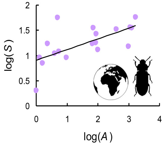
Figure 2.
Species-area relationship (SAR) for tenebrionid species (total richness) in Italian reserves.
Figure 2.
Species-area relationship (SAR) for tenebrionid species (total richness) in Italian reserves.

Figure 3.
Species-area relationship for tenebrionids in Italian reserves: (a) geophilous species, (b) xylophilous species, (c) widespread species, (d) endemic species.
Figure 3.
Species-area relationship for tenebrionids in Italian reserves: (a) geophilous species, (b) xylophilous species, (c) widespread species, (d) endemic species.

Figure 4.
Correlations (Pearson coefficient, r) between species richness (S: all species, G: geophilous, X: xylophilous, W: Widespread, E: endemic) and area, latitude, and elevation for tenebrionids in Italian reserves. * = p < 0.05, ** = p < 0.01, *** p < 0.001. A: area (in km2), Lat: Latitude (decimal degrees), Min: Minimum elevation (m), Max: Maximum elevation (m), Range: Elevational range (m), Mean: Mean elevation (m).

Figure 5.
Extinction rates (% of extinct species) expected on the basis of area reduction (% of area lost) for tenebrionids in Italian reserves. Solid line: expected rate from the species-area relationship. Dashed line: expected rate from multiple regression models.
Figure 5.
Extinction rates (% of extinct species) expected on the basis of area reduction (% of area lost) for tenebrionids in Italian reserves. Solid line: expected rate from the species-area relationship. Dashed line: expected rate from multiple regression models.

Figure 6.
Extinction rates (% of extinct species) expected on the basis of area loss (% of area lost) for tenebrionids in Italian reserves. (a) geophilous species, (b) xylophilous species, (c) widespread species, (d) endemic species. Solid lines: expected rates from the species-area relationship. Dashed lines: expected rates from multiple regression models. In panel (a) the two dashed lines refer to calculations based on two exponents: 0.187 (upper) and 0.104 (lower). Lack of dashed lines in panels (b,d) is because the best-fit multiple models included only area.


Table 1.
Number of species for various beetle groups in Italian reserves. Location, area, and elevation of reserves are also given. Res: Reserve number (reserves are numbered as in Figure 1), Lat: Latitude (decimal degrees), Long: Longitude (decimal degrees), Area: reserve size (km2), Min: Minimum elevation (m), Max: Maximum elevation (m), Range: Elevational range (m), Mean: Mean elevation (m). Tenebrionid groups: S: Total species richness, G = Geophilous species, X = Xylophilous species, W = widespread species, E = Endemic species.
| Res | Lat | Lon | Area | Min | Max | Range | Mean | S | G | X | W | E |
|---|---|---|---|---|---|---|---|---|---|---|---|---|
| 1 | 46.0208 | 11.9794 | 1 | 225 | 233 | 8 | 229 | 2 | 0 | 2 | 2 | 0 |
| 2 | 45.3117 | 8.9264 | 983 | 116 | 300 | 184 | 208 | 15 | 8 | 7 | 15 | 0 |
| 3 | 45.2011 | 10.7428 | 2.3 | 22 | 26 | 4 | 24 | 17 | 2 | 15 | 17 | 0 |
| 4 | 45.0403 | 11.2403 | 1.3 | 7 | 15 | 8 | 14 | 9 | 0 | 9 | 9 | 0 |
| 5 | 42.4006 | 11.2117 | 4 | 0 | 3 | 3 | 1.5 | 15 | 13 | 2 | 11 | 4 |
| 6 | 42.1614 | 13.8230 | 100 | 300 | 400 | 100 | 350 | 16 | 12 | 4 | 13 | 3 |
| 7 | 41.9769 | 12.6675 | 5.4 | 50 | 120 | 70 | 85 | 14 | 6 | 8 | 12 | 2 |
| 8 | 41.9325 | 15.1053 | 9.6 | 0 | 1 | 1 | 0.5 | 10 | 10 | 0 | 9 | 1 |
| 9 | 41.8050 | 15.8506 | 1700 | 0 | 950 | 950 | 456 | 64 | 35 | 29 | 57 | 7 |
| 10 | 41.7036 | 12.3754 | 70 | 0 | 70 | 70 | 35 | 45 | 24 | 21 | 35 | 10 |
| 11 | 41.3383 | 13.0383 | 88 | 0 | 541 | 541 | 270.5 | 37 | 23 | 14 | 27 | 10 |
| 12 | 40.9453 | 15.6339 | 66 | 650 | 1326 | 676 | 988 | 19 | 8 | 11 | 17 | 2 |
| 13 | 40.8211 | 14.4275 | 84.8 | 200 | 1281 | 1081 | 740.5 | 24 | 20 | 4 | 18 | 6 |
| 14 | 40.5881 | 15.7483 | 1.6 | 764 | 770 | 6 | 767 | 11 | 6 | 5 | 7 | 4 |
| 15 | 40.1753 | 16.6975 | 5 | 0 | 6 | 6 | 3 | 64 | 35 | 29 | 56 | 8 |
| 16 | 39.9650 | 16.2147 | 1100 | 800 | 2000 | 1200 | 1482 | 41 | 17 | 24 | 36 | 5 |
| 17 | 39.3197 | 16.5783 | 1250 | 1000 | 1900 | 900 | 1425 | 40 | 14 | 26 | 35 | 5 |
| 18 | 37.8858 | 13.9992 | 399.4 | 400 | 1979 | 1579 | 1189.5 | 42 | 22 | 20 | 33 | 9 |
Table 2.
Parameters of species-area relationships (SARs) for tenebrionids in Italian reserves. SARs were modelled using the linearized version of the power function: log(S) = log(c) + z log (A), where S is the species number, A is area, and c and z are fitting parameters. SE: standard error, t = Student’s t, p = probability, R2 = goodness of fit.
| Beetle group, R2 Values, and Estimated Parameters | Estimate ± SE | t | p |
|---|---|---|---|
| All tenebrionids (R2 = 0.416) | |||
| log(c) | 0.976 ± 0.121 | 8.094 | <<0.001 |
| z | 0.213 ± 0.063 | 3.374 | 0.004 |
| Geophilous species (R2 = 0.407) | |||
| log(c) | 0.613 ± 0150 | 4.075 | <0.001 |
| z | 0.261 ± 0.079 | 3.317 | 0.004 |
| Xylophilous species (R2 = 0.228) | |||
| log(c) | 0.721 ± 0.154 | 4.693 | <0.001 |
| z | 0.175 ± 0.080 | 2.172 | 0.045 |
| Widespred species (R2 = 0.440) | |||
| log(c) | 0.905 ± 0.114 | 7.911 | <<0.001 |
| z | 0.212 ± 0.060 | 3.544 | 0.003 |
| Endemic species (R2 = 0.195) | |||
| log(c) | 0.355 ± 0.145 | 2.449 | 0.026 |
| z | 0.149 ± 0.076 | 1.967 | 0.067 |
Table 3.
Best-fit models for the influence of area, latitude, and elevation on tenebrionid richness in Italian reserves. DF: degrees of freedom, R2adj: adjusted R2, AICc: corrected Akaike Information Criterion. Errors refer to standard errors. * = p < 0.05, ** = p < 0.01, *** p < 0.001.
Table 3.
Best-fit models for the influence of area, latitude, and elevation on tenebrionid richness in Italian reserves. DF: degrees of freedom, R2adj: adjusted R2, AICc: corrected Akaike Information Criterion. Errors refer to standard errors. * = p < 0.05, ** = p < 0.01, *** p < 0.001.
| Intercept | Area | Latitude | Minimum Elevation | Maximum Elevation | Mean Elevation | Elevational Range | DF | R2adj | AICc | |
|---|---|---|---|---|---|---|---|---|---|---|
| Total | ||||||||||
| 14.417 ± 3.823 (**) | 0.164 ± 0.047 (***) | −8.733 ± 2.333 (**) | −0.1312 ± 0.039 | 5 | 0.730 | 2.4 | ||||
| 15.143 ± 4.133 (**) | −8.575 ± 2.517 (**) | −0.162 ± 0.044 (**) | 0.173 ± 0.057 (**) | 5 | 0.699 | 4.3 | ||||
| Geophilous | 29.551 ± 10.335 (*) | −7.711 ± 2.695 (*) | 2.821 ± 0.535 (***) | −2.719 ± 0.506 (***) | 5 | 0.819 | 2.9 | |||
| 48.590 ± 9.024 (***) | 0.187 ± 0.049 (**) | −12.402 ± 2.391 (***) | −0.171 ± 0.040 (***) | 5 | 0.817 | 3.3 | ||||
| 31.222 ± 9.956 (**) | 0.104 ± 0.069 (ns) | −8.075 ± 2.592 (**) | 2.151 ± 0.678 (**) | −2.139 ± 0.619 (**) | 6 | 0.8341 | 4.6 | |||
| Xylophilous | 0.603 ± 0.167 (**) | 0.212 ± 0.079 (*) | 3 | 0.270 | 19.1 | |||||
| Widespread | 12.356 ± 4.049 (**) | 0.179 ± 0.050 (**) | −6.908 ± 2.470 (*) | −0.128 ± 0.042 (**) | 5 | 0.677 | 4.5 | |||
| Endemic | 22.353 ± 2.496 (***) | −13.436 ± 1.524 (***) | −0.214 ± 0.040 (***) | 0.173 ± 0.048 (**) | 5 | 0.876 | −10.7 | |||
| 21.607 ± 2.566 (***) | −13.004 ± 1.563 (***) | −0.199 ± 0.0373 (***) | 0.169 ± 0.169 (**) | 5 | 0.876 | −10.7 |
© 2020 by the author. Licensee MDPI, Basel, Switzerland. This article is an open access article distributed under the terms and conditions of the Creative Commons Attribution (CC BY) license (http://creativecommons.org/licenses/by/4.0/).
Share and Cite
MDPI and ACS Style
Fattorini, S. Conservation Biogeography of Tenebrionid Beetles: Insights from Italian Reserves. Diversity 2020, 12, 348. https://doi.org/10.3390/d12090348
AMA Style
Fattorini S. Conservation Biogeography of Tenebrionid Beetles: Insights from Italian Reserves. Diversity. 2020; 12(9):348. https://doi.org/10.3390/d12090348
Chicago/Turabian StyleFattorini, Simone. 2020. "Conservation Biogeography of Tenebrionid Beetles: Insights from Italian Reserves" Diversity 12, no. 9: 348. https://doi.org/10.3390/d12090348
Note that from the first issue of 2016, this journal uses article numbers instead of page numbers. See further details here.