Abstract
A lack of information regarding which ecological factors influence restoration success or failure has hindered scientifically based restoration decision-making. We focus on one headwater site to examine factors influencing divergent ecological outcomes of two post-mining stream restoration projects designed to improve instream conditions following 70 years of mining impacts. One project was designed to simulate natural stream conditions by creating a morphologically complex channel with high habitat heterogeneity (HH-reach). A second project was designed to reduce contaminants and sediment using a sand filter along a straight, armored channel, which resulted in different habitat characteristics and comparatively low habitat heterogeneity (LH-reach). Within 2 years of completion, stream habitat parameters and community composition within the HH-reach were similar to those of reference reaches. In contrast, habitat and community composition within the LH-reach differed substantially from reference reaches, even 7–8 years after project completion. We found that an interaction between low gradient and high light availability, created by the LH-reach design, facilitated a Chironomid-Nostoc mutualism. These symbionts dominated the epilithic surface of rocks and there was little habitat for tailed frog larvae, bioavailable macroinvertebrates, and fish. After controlling for habitat quantity, potential colonizing species’ traits, and biogeographic factors, we found that habitat characteristics combined to facilitate different ecological outcomes, whereas time since treatment implementation was less influential. We demonstrate that stream communities can respond quickly to restoration of physical characteristics and increased heterogeneity, but “details matter” because interactions between the habitats we create and between the species that occupy them can be complex, unpredictable, and can influence restoration effectiveness.
1. Introduction
Each year resource managers and agencies spend over one billion dollars on >5000 stream or river restoration projects in the United States alone [1]. Around the world, the rate of project implementation has increased dramatically since these figures were compiled [2]. Determining the common features of restoration projects deemed ecologically successful, however, has been thwarted by a lack of post-treatment assessments. For example, the National River Restoration Science Synthesis summary database shows that in the U.S., only 10% of stream restoration projects report any form of monitoring data [1,3]. Research-oriented stream restoration studies, particularly comparative or before-after studies, are needed to help guide design and implementation of stream restoration projects [3,4].
Answering the question “what works?” in stream restoration is critical to advancing restoration science and improving the degraded state of streams and rivers worldwide [5]. However, in stream restoration, as with restoration in general, many factors can contribute to ecological success or failure (e.g., [6,7,8]). Even the term “restoration success” is subjective and difficult to quantify. For our purposes, we define it as the degree of similarity to reference sites or pre-disturbance community composition. Restoration practitioners typically seek to achieve restoration success by altering degraded areas, commonly through improvements to habitat quality and quantity, as these factors are often the most readily manipulated means of improving conditions for target species or communities [9]. Many stream restoration projects, in particular, also seek to improve conditions through increasing habitat heterogeneity [10]. This is partly because many streams in need of restoration were simplified (i.e., channelized, armored, or regulated) for human purposes [11,12], but also because studies of intact ecosystems have shown positive relationships between particular species, or species diversity as a whole, and habitat complexity or heterogeneity [13]. The ecological effectiveness of intentionally increasing habitat heterogeneity has been mixed in stream restoration studies [10] and increasing habitat heterogeneity does not guarantee use by a particular target species or establishment of desired (pre-disturbance) community composition.
The ecological success of restoration actions can be further influenced by often overlooked factors such as species’ traits (e.g., dispersal ability, generation time, response to disturbance, specializations), biogeography (e.g., distance and connectivity to source populations), successional processes (e.g., time since project completion), and complex interspecific interactions such as facilitation, predation, or competition [14]. Since these factors are largely context specific, comparative- or case-studies of restoration projects situated in similar ecological contexts may provide a valuable means of elucidating how these potential drivers combine to influence restoration outcomes [15]. Although broad-scale, replicated studies can provide inference for quantifying success rates of certain restoration approaches and for determining “what works” and “where” (e.g., [16]), drawing more detailed mechanistic conclusions about drivers of restoration success or failure is challenging for such studies [17,18]. Thus, restoration case studies fill an important role in enhancing understanding of the ecological complexities of restoration outcomes.
Here, we provide a multi-year, multi-trophic level, comparative study of two post-mining restoration projects implemented on the same headwater stream. Differences in the designs of these projects allowed us to investigate the relative importance of habitat characteristics and time since treatment implementation, while controlling (to the extent possible in a natural experiment) for habitat quantity, species’ traits (i.e., equivalent colonizing species pool), and biogeographic factors. To this end, we compared habitat conditions and biotic communities in two stream restoration reaches to an undisturbed reference reach upstream from any mining activities and to an unrestored downstream reach. Our goals were to determine the initial ecological effects of the two stream restoration strategies and to elucidate potential mechanisms contributing to different ecological outcomes. We hypothesized that habitat characteristics would ultimately have the greatest direct influence on the biotic communities in these stream reaches, whereas time since restoration completion would be relatively unimportant if quality habitat was lacking.
2. Materials and Methods
2.1. Study Area
The Stibnite Mine is located at 2034 m elevation in the Salmon River Mountains, Idaho, U.S.A. (Figure 1). Surrounding forests are dominated by various fir species and lodgepole pines. Summers are warm and dry, with most annual precipitation falling as winter snow. Meadow Creek, a third order stream with a moderate (11 m/km) gradient, runs through the site and has been heavily altered by mining activities since the 1930’s [19,20]. In addition to being proposed by the U.S. Environmental Protection Agency as a “Superfund” site, Meadow Creek is designated critical habitat for three salmonid fish species listed as Threatened under the Endangered Species Act. As a headwater stream, contaminant inputs are transported downstream into the Salmon River, the longest free-flowing river system in the contiguous U.S. (Figure 1 inset).
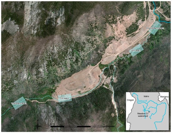
Figure 1.
Stibnite Mine site, with Meadow Creek flowing northeast into the East Fork of the South Fork Salmon River (at top right). Over 3.2 km of mine tailings extend from the low habitat heterogeneity (LH-reach) through the high habitat heterogeneity (HH-reach). Boxes indicate 250 m study reaches. Inset shows the Meadow Creek watershed and its location in the headwaters of the Salmon River system in central Idaho, an area designated as critical habitat for three salmonid fish species listed as Threatened under the Endangered Species Act.
To improve in-stream habitat conditions and reduce heavy metal and sediment contaminants derived from mine tailings [19], two stream restoration projects were implemented. One project, implemented in 2005, was designed to closely resemble nearby stream habitats and to achieve high heterogeneity (HH-reach). This involved excavating a new channel adjacent to mine tailings, creating meanders, and restoring historic gradients, substrates, microhabitats, and riparian plants (Appendix A, Figure A1). Another project, implemented in 1999, consisted of excavating a straight flowing, armored, low-gradient stream channel through mine tailings and installing a sand filter (Figure A2). This resulted in a stream reach with somewhat unique habitat characters and relatively low heterogeneity in most variables examined (LH-reach; Table 1). The reaches are the same length (1.4 km) and are separated by 1.7 km. Each reach is approximately 450 m downstream, and 500 m upstream, from tributaries that provide potential colonizing species (Figure 1). See Appendix A for additional study area and restoration details.

Table 1.
Habitat results by year of sampling and reach. For quantitative variables, values reported are mean ± S.E. Groups with the same letter (i.e., a–e) are not significantly different (α = 0.05) according to Duncan’s Multiple Range Test. For categorical variables, the proportion of transects in each categorical level is reported by group. Variable names are capitalized.
2.2. Study Design
In addition to the HH- and LH-reaches, we sampled an unrestored reference reach downstream of the restoration projects (Downstream-reach, Figure A3) and an undisturbed upstream reference reach (Upstream-reach; Figure A4). Due to the directional flow, the three lower reaches are not independent and could be influenced by conditions in higher reaches of the stream. However, these reaches have different tributaries downstream and upstream from them and we focus on structural habitat conditions (rather than water chemistry and contaminants) that are less likely to have cross-reach independence issues. In late July 2006 and 2007, we sampled 10 belt-transects in 250 m sections of each study reach. Belt-transects were placed at 25 m intervals in each section, with random off-sets of ±2 m. Each belt-transect extended across the wetted width of the stream and upstream for 1 m. Pre-restoration data on habitat and communities were not available except for fish in two reaches. Therefore, we did make opportunistic use of these data since they were available. Pre- and post-restoration water chemistry and site contaminant data are provided in Dovick et al., 2016 and 2020 [19,20], and were thus not presented here. We do note, however, that metalloid contaminant levels in sediment, water, and biotic samples generally increased with current direction (i.e., greatest in Downstream-reach, next greatest in HH-reach, followed by LH-reach, and Upstream-reach), both before- and after restoration in 2005.
We sampled in two different years due to the dynamic nature of streams in this disturbance-prone landscape. Wildfires, debris flows, and high interannual variability in peak spring runoff levels are common. Thus, results obtained from streams sampled in 1 year can differ substantially from those obtained in a subsequent year [21,22]. We sampled and compared data across two years to provide a means of reducing the chances of spurious conclusions being drawn from a single year’s data.
2.3. Stream Habitat Sampling
At each belt-transect, we recorded wetted width, average depth, current velocity (CURRENT), percent of transect covered by sediment (SEDIMENT), substrate size (SUBSTRATE), and substrate embeddedness (EMBEDDEDNESS) as in [21]. We measured the percent of each belt-transect covered by large woody debris (LWD; >5 cm diameter) and the volume of organic debris dislodged during kick sampling (ORGANIC; wood < 5 cm diameter and leaf litter). We also recorded the percent of each belt-transect covered by riparian vegetation (COVER) and the percent of the shoreline with undercut bank morphology (UNDERCUT). The microhabitat type of each belt-transect was classified as having no surface agitation (GLIDE), agitation but no whitewater (LOWGRAD), or whitewater (HIGHGRAD). The substrate mobility within each belt-transect was rated, relative to the effort required to dislodge benthic rocks, as: immovable when kicked (SOLID), kicking effort required (RESISTANT), and movement when stepped on (LOOSE).
We used Solar Pathfinder equipment and digital photography to provide year-round, transect-specific solar data (Solar Pathfinder Assistant version 1.1.5, 2006). June–August average light availability (kW·m2·hr−1; LIGHT) was used in analyses.
Water temperature was recorded hourly (HOBO data loggers, Onset Computer Corp., Bourne, MA, USA) in two locations: where water entered the LH-reach and where it exited the HH-reach. For each location, we determined the number of hours each summer, where water temperatures were ≥16 °C (WATERTEMP) [21].
2.4. Stream Community Sampling
We collected, dried, and weighed all autochthonous primary production (PERIPHYTON) that was dislodged while taking each Surber sample (see below). We recorded whether the dominant epilithic macro- or microphyte in each belt-transect was biofilm, filamentous algae, moss, or cyanobacteria colonies (Nostoc sp.).
Surber samples (0.10 m2, 500 µm mesh) were collected in the thalweg of alternate belt-transects (50-m apart) for a total of 5 samples per reach per year. Benthic macroinvertebrates were keyed to genus (family for Chironomidae and order for Oligochaeta) using Merritt and Cummins (1996) [23]. We calculated macroinvertebrate summary metrics including total density (DENSITY), density of each genus, taxonomic richness (RICHNESS), and evenness (EVENNESS; inverse of dominance) for each sample.
In each belt-transect, we kick-sampled for Rocky Mountain tailed frog larvae (Ascaphus montanus), which were captured in D-frame nets at the downstream edge of the belt-transect [21]. For each reach and year, we calculated the proportion of belt-transects occupied by larvae. We also recorded incidental observations of adult tailed frogs.
Snorkeling surveys were conducted by the Payette National Forest in the Downstream-reach and in the HH-reach prior to relocation of the stream channel in 2005, and again after restoration in 2006 and 2007. Fish counts were made by species and life stage. We used these data to calculate the number of fish per meter surveyed and report the species composition for each reach in each year. We supplemented snorkeling data with observational data at all 10 belt-transects per reach in both years and we report the proportion of transects where fish were detected by reach and year. We report naïve occupancy rates rather than rates adjusted for detection probability.
2.5. Data Analysis
We tested for significant differences in response variables among combinations of four reaches and two years, which resulted in comparisons among eight groups (GROUP). This approach allowed us to quantify differences between reaches and changes through time in a manner that was consistent with the approach required for multivariate analyses discussed below. Untransformed univariate quantitative response variables were analyzed using general linear modeling (GLM) and a post-hoc, Duncan’s Multiple Range Test after checking for compliance with model assumptions. Categorical habitat variables were analyzed using chi-square tests (SAS 9.0.1, SAS Institute Inc., Cary, NC, USA). To assess habitat heterogeneity differences between GROUPs, we examined relative standard error (RSE = standard error/mean) values for each individual quantitative variable measured by GROUP. RSE provides an index of heterogeneity by relativizing the within GROUP variability for a given habitat variable by the mean value of that variable for all transects, with values > 0.20 being considered relatively high in ecological studies [24]. We further compared the mean RSE of all nine quantitative habitat variables for each GROUP to provide an overall score of each reaches’ relative heterogeneity.
To test for community-level differences between GROUPs, macroinvertebrate samples were analyzed using Multi-Response Permutation Procedure (MRPP) in PC-ORD [25]. See Appendix B for details on this and subsequent multivariate analyses. We performed indicator species analyses (ISA) to determine which macroinvertebrate genera were significantly associated with, or indicative of, a particular GROUP [25]. Relationships between macroinvertebrate community composition and habitat or treatment variables were analyzed using nonmetric multidimensional scaling (NMS) ordination performed on genera density data.
To determine which habitat variables influence the prevalence of the dominant macroinvertebrate taxon, we used nonparametric multiplicative regression (NPMR) in HyperNiche 2.11 software [26]. This approach allowed us to model the density of the dominant taxon as a function of non-linear, multiplicatively interacting combinations of habitat variables [27].
3. Results
3.1. Stream Habitat
Habitat conditions varied predominantly among reaches, with fewer changes between years. There was a significant difference between reaches in the amount of microhabitat types (Table 1; χ2 = 17.3, n = 80, d.f. = 6, p = 0.008). The HH-reach contained mostly LOWGRAD, whereas the LH-reach contained largely GLIDE habitat. The reference reaches contained mostly LOWGRAD but had comparatively higher proportions of HIGHGRAD and GLIDE habitats. CURRENT differed significantly across both reach and sampling year. Within each year, the LH-reach had significantly slower CURRENT than the other three reaches (approximately half that of the Downstream- and HH-reaches; Table 1). Within each year, the HH-reach had more variable CURRENT than the Downstream- and LH-reaches.
Substrate characteristics varied among reaches and sampling year (Table 1). Average SUBSTRATE was smallest in the HH- and Upstream-reaches. SUBSTRATE did not change significantly from year to year within any reach except in the HH-reach, where the average size increased. SEDIMENT was higher in the LH-reach than in the other three reaches. The HH-reach had the least embedded substrate in both years, whereas the LH-reach had the most embedded substrate in 2006 (Table 1). Substrate mobility differed significantly among reaches (Table 1; χ2 = 34.8, n = 80, d.f. = 6, p = 0.0001). The HH- and Upstream-reaches had substrate that was LOOSE or RESISTANT, whereas the LH-reach substrate was more often RESISTANT. In both years, the HH-reach had higher between-transect variability than the LH-reach for most of the substrate variables examined (Table 1).
The amount of in-stream vegetative material (LWD, ORGANIC), riparian vegetation (COVER), and undercut banks (UNDERCUT) were greater in the Upstream-reach than in the other three reaches. The Downstream-reach had significantly more COVER than the HH- and LH-reaches, but did not have significantly more LWD, ORGANIC, or UNDERCUT than either of the restoration reaches. The LH-reach generally lacked each of these habitat elements (Table 1). LIGHT differed significantly among reaches, but not years. The HH- and LH-reaches each received around 7 kW·m2·hr−1. The Downstream-reach received 65% less- and the Upstream-reach received 43% less LIGHT than the two restoration reaches because of riparian shading (Table 1). Water temperatures increased as water flowed through the two restoration reaches (Table 1).
Based on RSE analysis of quantitative habitat variables, the HH-reach had greater heterogeneity than the LH-reach in both years (Appendix C Table A1, Figure A5). In 2006, substrate size, substrate embeddedness, and riparian cover were the primary drivers in this difference in heterogeneity. Whereas, by 2007, variability in substrate embeddedness was similar among the two reaches and sediment load variability was found to be greater in the HH-reach, as were substrate size, LWD, ORGANIC, and COVER (Table A1). Across all quantitative habitat variables, the average RSE was 57–61% greater in the HH-reach than in the LH-reach, depending on year of sampling. Average RSE values increased between 2006–2007 in all reaches (except the Downstream-reach), likely due to higher peak stream flows that spring. By 2007, average RSE values in the HH-reach were significantly greater than those of the other three reaches (Appendix C Figure A5), mainly because of increases in the diversity of CURRENT, LWD, and ORGANIC, as these habitat elements began to appear in this reach.
3.2. Periphyton
PERIPHYTON differed significantly by reach, but not by year (Table 2). PERIPHYTON was approximately three times greater in the LH-reach than in the Upstream-reach, which in turn, had significantly more PERIPHYTON than the Downstream- and HH-reaches. Similar to PERIPHYTON, the dominant epilithic macro- or microphyte differed substantially by reach (χ2 = 127.8, n = 80, d.f. = 9, p < 0.0001 (Table 2). In the Downstream- and HH-reaches, diatom/microalgae (FILM) was the dominant epilith in all belt-transects in both years. Cyanobacteria colonies (NOSTOC), and to a lesser extent filamentous ALGAE, dominated in the LH-reach, whereas FILM dominated in the Upstream-reach and MOSS was subdominant (Table 2).
Table 2.
Biotic results by year of sampling and reach. For quantitative variables, values reported are mean ± S.E. Groups with the same letter (i.e., a–d) are not significantly different (α = 0.05) according to Duncan’s Multiple Range Test. For categorical variables, the proportion of transects in each categorical level is reported by group. Variable names are capitalized.
3.3. Macroinvertebrates
Benthic macroinvertebrate communities in the HH- and Downstream-reaches each changed significantly between years of sampling (T < −1.6; A > 0.05; p < 0.05). The LH-reach reach did not change significantly between years (T = −1.54; A = 0.04; p = 0.08), nor did the Upstream-reach (T = −1.34; A = 0.02; p = 0.09).
NMS ordination produced a two-axis solution (instability = 0.00000, 54 iterations, stress = 10.3, p = 0.004), representing 66.6% of the variance in the original data. Samples fell into two clusters, one cluster containing samples from the LH-reach (both years) and the other cluster containing samples from the other three reaches, except for one outlier from the LH-reach (discussed below). Within the larger cluster, the Downstream- and HH-reaches were similar in both years (Figure 2). These reaches were positively correlated with high WATERTEMP and LIGHT and negatively correlated with COVER, small substrate, and PERIPHYTON. The Upstream-reach did not change from 2006 to 2007 and was associated with high COVER, small substrate, and low LIGHT. CURRENT was positively correlated with samples from these three reaches. Samples from the LH- reach were distinct and did not vary between years (Figure 2). Low CURRENT, high LIGHT, and high PERIPHYTON were associated with this reach. One outlying point from the LH-reach (in 2006) clustered with samples from the other reaches. This sample was collected in a transect that had a current velocity of 74 cm/s, which was 50% greater than the average current velocity in that reach and equal to the average current velocity in the HH-reach.
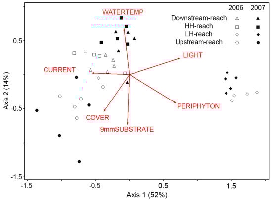
Figure 2.
Nonmetric multidimensional scaling (NMS) biplot of five Surber samples per reach per year (n =40) in two-dimensional genera space. Samples plotted closer together have more similar macroinvertebrate communities. Percent variance represented by each axis is given in parentheses. Current velocity (CURRENT) is most strongly correlated with Axis 1 (r2 = 0.32). Water temperature (WATERTEMP) is positively related (r2 = 0.41) and small substrate size (9 mmSUBSTRATE) is negatively related (r2 = 0.41) to Axis 2. Riparian canopy cover (COVER), periphyton biomass (PERIPHYTON), and solar availability (LIGHT) are related to both axes (r2 > 0.23 for both axes).
Macroinvertebrate density (DENSITY) was significantly different among reaches and years. Chironomid taxa had a strong influence on DENSITY (Figure 3). Including Chironomids, DENSITY in the LH-reach was an order of magnitude greater than that of any other reach. The thousands of Chironomids found in the LH-reach were found exclusively living encased within Nostoc parmelioides cyanobacteria colonies (Appendix D). Excluding Chironomids from density calculations results in a different pattern. Non-Chironomid DENSITY in the HH-reach was 3.3-fold greater than in the LH-reach in 2007 (Figure 3; Table 2). Non-Chironomid DENSITY was significantly lower in the LH-reach than in the Downstream- and HH-reaches.
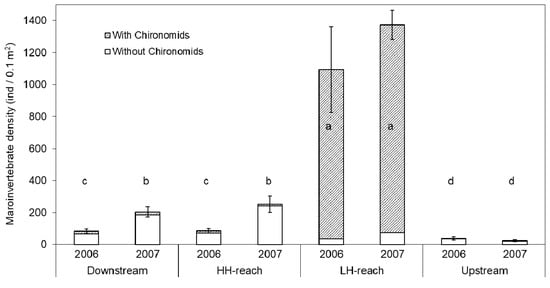
Figure 3.
Average macroinvertebrate density (DENSITY), including and excluding Chironomids, from five Surber samples per reach per year. Error bars show ± 1 SE for total DENSITY only. Groups with the same letter (i.e., a–d) are not significantly different (based on total DENSITY; α = 0.05) according to Duncan’s Multiple Range Test.
Taxonomic RICHNESS ranged from 12.8 in the HH-reach to 8.0 in the Upstream-reach (both in 2007). These were the only two GROUPs that differed significantly (Table 2). EVENNESS however, differed significantly across reaches and was greater in the Upstream-reach than in than the two restoration reaches. The Downstream- and HH-reaches did not differ in EVENNESS, but had significantly greater EVENNESS than the LH-reach (Table 2).
Indicator Species Analysis identified 10 taxa with significant indicator values for at least one reach in at least one year (Table 3). In total, three taxa, the mayfly Drunella, the stonefly Yoroperla, and Chironomids, were characteristic of a particular reach in both years. In general, taxa that are periphyton scrapers were indicative of the Downstream- and HH-reaches, whereas a Nostoc colony miner/macroalgae chewer was associated with the LH-reach. A shredder/scraper was associated with the Upstream-reach. Mobile and unprotected (i.e., by a rock or plant material casing) taxa were associated with the Downstream-, HH-, and Upstream-reaches.
Table 3.
Indicator Species values (percentage of a perfect indication) for macroinvertebrate taxa. Taxa shown have an indicator value significantly greater (α = 0.05) than values generated by 1999 Monte Carlo simulations, in at least 1 year of sampling.
The density of Chironomid-Nostoc mutualists (Figure A5) across transects in all reaches was best explained by a non-linear interaction between CURRENT and LIGHT, which explained 92% of the variation in mutualist density (Figure 4; n = 20, N* = 4.04, xR2 = 0.92, p = 0.024). Mutualist density was high in transects where CURRENT was low and LIGHT was high, conditions found in the LH-reach. However, mutualist density was low where both CURRENT and LIGHT were high (conditions found in Downstream- and HH-reaches). High CURRENT and low LIGHT, as was observed in the Upstream-reach, resulted in intermediate densities. For CURRENT and LIGHT respectively, tolerance was 0.106 and 0.886 (both 20% of the range of the variable) and sensitivity was 0.804 and 0.838.
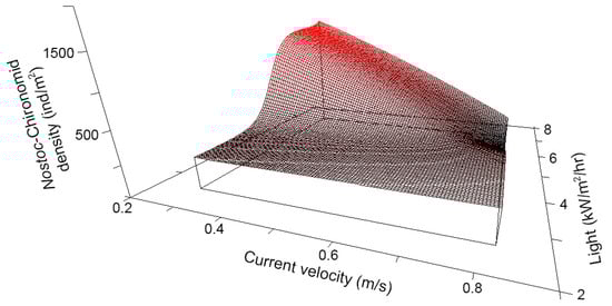
Figure 4.
Nonparametric multiplicative regression (NPMR) modeled Chironomid-Nostoc mutualist density versus current velocity and light availability. Model is based on density data from 20 Surber samples collected in 2006 and explains 92% of the variation in the empirical data.
3.4. Amphibians
In 2006, tailed frog larvae occupied 10% of transects in the HH-reach and no transects in the LH-reach (Figure 5). Occupancy rates were at least twice as high in the Downstream- and Upstream-reaches compared with the HH-reach. In 2007 however, the HH-reach had the highest larval occupancy rate, which was > 30% higher than that of the Downstream- and Upstream-reaches. Occupancy in the Downstream- and Upstream-reaches decreased by about 50% from the previous year and again, no tailed frog larvae were detected in the LH-reach. Adult tailed frogs were observed only in the Upstream- and Downstream-reaches (not shown).
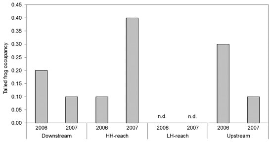
Figure 5.
Proportion of belt-transects occupied by tailed frog larva in each reach and year. No larvae were detected in the LH-reach (n.d.).
3.5. Fish
The number of fish per meter surveyed more than doubled in the HH-reach from pre-restoration levels, whereas numbers remained relatively constant in the Downstream-reach over the same years (Figure 6). Prior to restoration, westslope cutthroat trout (Oncorhychus clarki) and steelhead (O. mykiss) were observed in the Downstream-reach, but only westslope cutthroat trout were observed in the former channel flowing through the HH-reach area. After 1- and 2-years post-restoration, westslope cutthroat trout, steelhead, and bull trout (Salvelinus confluentus) were observed in the HH-reach, whereas only westslope cutthroat trout were observed in the Downstream-reach. The Upstream- and LH-reaches were not surveyed by Payette National Forest crews.
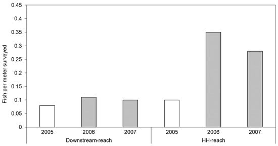
Figure 6.
Number of fish (all species and size classes) per meter counted during snorkeling surveys. Data from 2005 (unshaded bars) were collected prior to initiation of restoration actions on the HH-reach.
During belt-transect sampling of all four reaches, the naïve fish occupancy rate in 2006 was 0.30 in the HH-reach (i.e., fish detected in 30% of transects) and 0.10 in the LH-reach. Downstream- and Upstream-reaches had occupancy rates of 0.10 and 0.30, respectively. In 2007, occupancy rates declined slightly to 0.20 in the HH-reach and to 0.10 and 0.20 in the Downstream- and Upstream-reaches, respectively. The LH-reach was the only area with no fish detected in 2007 (naïve occupancy rate = 0.00).
4. Discussion
4.1. Effects of Restoration Strategy on Stream Habitat
A companion study at this site found that these restoration actions were effective in reducing arsenic and antimony contamination, especially where sand filters were installed for ground water filtration, although contaminant levels remained elevated and there was evidence of substantial bioaccumulation [19]. However, we found that the two restoration strategies resulted in pronounced differences in stream habitat conditions. The more holistic restoration approach used in the HH-reach resulted in greater habitat heterogeneity and in overall habitat conditions that were more similar to reference reach conditions within 2 years of project completion, despite having substantially greater metalloid concentrations in sediment, water, and biotic samples than concentrations observed in the LH-reach [19]. With a restoration emphasis on contaminant and sediment reduction, habitat conditions in the LH-reach were dissimilar to reference conditions even after 8 years since project completion. The proportion of different microhabitat types, substrate characteristics, and perhaps most importantly, current velocity were key differences between HH- and LH reaches. However, other habitat components such as large wood, riparian cover, and undercut bank morphology were generally lacking in each restoration reach when compared to reference conditions, similar to findings from other stream restoration studies (e.g., [16]). Similar to what Bernhardt and others [3] found, there was not a substantial cost difference between the successful and less successful habitat restoration projects (Payette National Forest unpublished data), but the habitat differences we observed resulted in considerably different conditions for in-stream communities.
4.2. Effects of Stream Restoration Strategy on Stream Community
Periphyton community composition and biomass in the two restoration reaches were dramatically different despite equal solar energy availability. Periphyton, including epilithic moss, has been shown to provide important post-restoration refugia and habitat as macroinvertebrates colonize new benthic surfaces [28,29]. The dominant periphyton community in the HH-reach (diatom/microalgae) was similar to that of reference reaches and it supported an abundant assemblage of predominantly scraper macroinvertebrates. In contrast, benthic substrates in the LH-reach were almost completely covered by Nostoc parmelioides, a colonial cyanobacteria that was far less abundant in the other study reaches and in 13 other streams in the vicinity [21,22]. Our habitat model shows that the cause of this dominance was likely an interaction between light availability and current velocity, conditions resulting from restoration actions (discussed further below). Past studies have implicated these two factors separately in influencing Nostoc sp. performance by controlling photosynthetic rate [29] and the rate of gas exchange [30], respectively. As the autochthonous base of the stream food web and as a structural habitat component, this difference in periphyton community may explain the observed differences in higher trophic-level organisms in these reaches [31,32].
Despite a lack of riparian cover, large woody debris, and complex bank morphology, the macroinvertebrate community in the HH-reach was similar to communities of reference reaches, likely because of similar substrate and current conditions. This is in contrast to some studies which have found that restoring structural features does not necessarily translate into improvements in macroinvertebrate community composition (e.g., [33]). In the LH-reach, however, low current velocity from the grading done during the restoration process and high light availability from a lack of riparian canopy cover resulted in dominance of the LH-reach by Chironomid larvae of the Cricotopus genus. These specialists live within colonies of the cyanobacteria Nostoc parmelioides, which provide the Chironomid larvae with food, oxygen, and protection from predation by other macroinvertebrates and fish [34,35]. The macroinvertebrates associated with the HH-reach, on the other hand, tended to be unprotected by Nostoc refugia or by rock casings. Others have shown that, in California streams, “unprotected” macroinvertebrates were more bioavailable to secondary consumers than macroinvertebrates which were protected by casings [36]. Therefore, habitat conditions in the LH-reach may ultimately result in lower autochthonous energy for predatory macroinvertebrates and fish, at least until Chironomid larva pupate and emerge from their hosts. These differences could potentially lead to alternative stable states in these two restoration reaches, with long-term consequences to restoration outcomes.
We were surprised that tailed frog larvae colonized the HH-reach within a year of channel relocation and that their occupancy rate surpassed that of reference sites within 2 years because tailed frogs are generally considered to be sensitive to disturbance and warm temperatures [37]. We cannot differentiate between tadpoles that immigrated from connected source habitats and those that hatched within the HH-reach, but the availability of biofilm periphyton (preferred food source) and interstitial spaces (cover from predators) within the unconsolidated substrate may explain the rapid colonization and high occupancy rate in the HH-reach [37]. No tailed frog larvae were observed in the LH-reach, probably because of the low gradient and slow current [38,39] created by the restoration project. The abundance of epilithic Nostoc colonies likely also limited tailed frog use in the LH-reach (an indirect effect of restoration approach), because Nostoc are unpalatable to most stream herbivores [40,41] and because tailed frog larvae have evolved a specialized feeding mechanism for stream-living, whereby they attach to rocks using suction and feed via scraping periphyton from rock surfaces [42].
Predatory fish density and richness (Family Salmonidae) both increased in the HH-reach following restoration, perhaps due to high densities of bioavailable macroinvertebrates and increased habitat quality. We found that four genera of bioavailable macroinvertebrates (three scraper mayflies and a predatory stonefly) were significantly associated with riffle habitats of the HH-reach. Compared with other reaches, the benthic substrate in the HH-reach was less embedded and more loosely anchored, while the stream was wider and shallower, creating a greater diversity of current velocities, microhabitats, and macrohabitats (i.e., pools, riffles). In contrast, the LH-reach had the lowest abundance of bioavailable macroinvertebrates and the lowest variability in habitat parameters (i.e., heterogeneity), probably resulting in low fish diversity and occupancy rates, as heterogeneity is important for fish species during different seasons and life history stages [43,44].
4.3. Mechanisms Contributing to Different Ecological Outcomes
Our analyses suggest that the primary differences in biotic community responses to these restoration projects are related, either directly or indirectly, to stream gradient, substrate, and light availability. The low gradient of the LH-reach resulted in low current velocities which likely caused sediment to settle and embed the rock substrate. We found that these conditions, along with high light availability, favored the mutualistic interaction between Nostoc parmelioides and Chironomid larva. The mutualists dominated the benthic community, resulting in poor habitat conditions for tailed frog larvae, most macroinvertebrate genera, and reduced available prey resources for salmonids. These findings suggest that a combination of habitat qualities was the main, direct determinant of differences in ecological outcome of the two restoration projects.
While the more heterogeneous project was more ecologically successful, and thus at a minimum, increasing heterogeneity did not hinder restoration effectiveness, we found inconclusive evidence that habitat heterogeneity itself was the primary driver, as habitat heterogeneity is scale-dependent and varies across space, time, and species. For example, where habitat characteristics in the LH-reach did resemble those of other reaches, as was the case in one outlying transect, periphyton and macroinvertebrate community composition was indistinguishable from that of the other reaches. Ostensibly, increasing the number of these microhabitats within the LH-reach would have increased habitat heterogeneity, and perhaps the entire community would have shifted to resemble the HH-reach, but it would still be difficult to determine whether habitat characteristics or heterogeneity itself was responsible. This may be one reason why past restoration studies have found varying effects of increasing habitat heterogeneity on fish [45,46,47] or macroinvertebrate biodiversity [33]. Time since completion of these projects also did not appear to be important in determining restoration success, as the more recent project was more ecologically successful. The concept of habitat restoration is predicated around the notion that, through successional processes, restored habitats will become more similar to natural conditions with time [9], otherwise restoration actions would need to be continually applied to maintain desired conditions. Likewise, biogeography, the traits of potential colonizers, and elevated contaminant levels were also relatively unimportant in determining ecological success of these two projects since the restoration reaches had similar potential colonizing species, similar connectivity and distance to sources of these species, and the reach with greater post-restoration metalloid concentrations [19] was more ecologically successful.
5. Conclusions
Determining which factors influence the outcome of management actions aimed at improving habitat or maintaining populations is a central question in restoration ecology. Despite the importance of this question, it is rarely answered empirically following project implementation [18], especially in stream or river habitats [3,48]. We found that habitats and communities in restoration sites can quickly (within 1–2 years) resemble reference conditions when holistic restoration techniques are used, when colonizing species are nearby, and when those species are adapted to dynamic environments. However, our findings suggest that “details matter” and in stream restoration, restoring physical characteristics such as historic gradients, may provide a foundation for an ecologically successful project. Interactions between the habitats that we create and between the species that occupy them can be complex, unpredictable, and can influence restoration effectiveness. Understanding and planning for this uncertainty will help guide restoration decisions.
Author Contributions
Conceptualization, R.S.A. and D.S.P.; methodology, R.S.A. and D.S.P.; formal analysis, R.S.A.; investigation, R.S.A. and D.S.P.; data curation, R.S.A.; Writing—Original draft preparation, R.S.A.; Writing—Review and editing, R.S.A. and D.S.P.; funding acquisition, D.S.P. All authors have read and agreed to the published version of the manuscript.
Funding
This research was funded by USDA Forest Service, Payette National Forest and the U.S. Geological Survey, Forest and Rangeland Ecosystem Science Center.
Institutional Review Board Statement
The study was conducted according to the guidelines of the Declaration of Helsinki, and approved by the Institutional Review Board (or Ethics Committee) of Boise State University (Institutional Animal Care and Use Committee (IACUC) Permit #692-AC11–013).
Informed Consent Statement
Not applicable.
Data Availability Statement
The data presented in this study can be found at https://www.sciencebase.gov/catalog/ by searching for the article title information.
Acknowledgments
USDA Forest Service, Payette National Forest provided critical information and we thank Mary Faurot and Gina Bonaminio for supporting our efforts. This work was conducted under the Research Collecting Permit #030716 from the Idaho Department of Fish and. Any use of trade, product, or firm names is for descriptive purposes only and does not imply endorsement by the U.S. Government.
Conflicts of Interest
The authors declare no conflict of interest. The funding agency provided fish data and information on the two restoration projects, but had no role in the design of the study; in the collection, analyses, or interpretation of other data; or in the writing of the manuscript, or in the decision to publish the results.
Appendix A
The Stibnite Mine has been a source of sediment, heavy metal (arsenic, antimony, cadmium, lead, mercury, selenium) and cyanide contamination in Meadow Creek and the South Fork Salmon River system for decades. This central Idaho mine produced antimony, tungsten, and gold beginning in the 1930s. Runoff and leaching of contaminants has been a chronic problem for resource managers, as Meadow Creek flows through approximately 3.2 km of mine tailings (Figure 1 of article). Water samples collected by Idaho Department of Environmental Quality on a semi-annual basis from the 1980s to 2000, showed concentrations of arsenic and cyanide that consistently exceeded the Environmental Protection Agency’s (EPA) aquatic chronic level, and often exceeded the aquatic acute level for stream-dwelling organisms (Woodward-Clyde 1998). In addition to contaminants, data collected by the Payette National Forest Fisheries Program indicate that Meadow Creek was a primary source of sediment affecting downstream aquatic habitats (M. Faurot, Payette National Forest, unpublished data). In 2001, the EPA proposed to add the Stibnite/Yellow Pine Mining Area to its National Priorities List of the nation’s most contaminated hazardous waste sites; “Superfund” sites that are targeted for investigation and cleanup under the Comprehensive Environmental Response, Compensation, and Liability Act (CIRCLA).
The U.S. Department of Agriculture Forest Service, in cooperation with the EPA and the responsible mining company, initiated two stream restoration projects to reduce human exposure to contaminants in water and fish, and to improve in-stream habitat. The first project (LH-reach), completed in 1998, involved excavating a straight flowing, low gradient stream channel to a depth below the level of the mine tailings, installing a sand filter between the tailings and stream, and armoring the channel bottom and streamside with rock substrate (Woodward-Clyde 1998). This low gradient portion of the channel extends for 1.4 km and then flows into an extremely high gradient section of channel that extends for 0.2 km. The second restoration project (HH-reach) was completed in 2005 in a 1.4 km reach downstream from the first project. The stream channel in this second reach was excavated adjacent to the mine tailings and was constructed with meanders, a moderate gradient, alternating pools and riffles, large wood debris, intermediate benthic substrate sizes, and a riparian zone enriched with transplanted topsoil and planted with approximately 38,000 tree cuttings and seedlings. Just downstream of this restoration project, the newly constructed stream rejoins the original stream channel (Downstream-reach).
The South Fork of the Salmon River and its tributaries, including Meadow Creek, are designated critical habitat for three species listed as threatened under Endangered Species Act: Snake River chinook salmon (Oncorhynchus tshawytscha), Snake River steelhead (Oncorhynchus mykiss), and Columbia River bull trout (Salvelinus confluentus). Westslope cutthroat trout (Oncorhynchus clarki), a special status species, also occurs in the drainage. Rocky Mountain tailed frogs (Ascaphus montanus) occur in most streams in the area.
Woodward-Clyde. (1998) Stibnite area site characterization report. Unpublished report prepared for The Stibnite Area Site Characterization Voluntary Consent Order Respondents.

Figure A1.
HH-reach in summer 2007. Photo by David Pilliod.
Figure A1.
HH-reach in summer 2007. Photo by David Pilliod.


Figure A2.
LH-reach in summer 2007. Photo by Robert Arkle.
Figure A2.
LH-reach in summer 2007. Photo by Robert Arkle.


Figure A3.
Downstream-reach in summer 2007. Photo by Robert Arkle.
Figure A3.
Downstream-reach in summer 2007. Photo by Robert Arkle.


Figure A4.
Upstream-reach in summer 2012. This area burned in 2007 after field sampling was completed. Photo by Robert Arkle.
Figure A4.
Upstream-reach in summer 2012. This area burned in 2007 after field sampling was completed. Photo by Robert Arkle.

Appendix B
For MRPP analysis, we report a test statistic (T), with increasingly negative values indicating greater multivariate differences between GROUPS, an effect size statistic, A (0 to 1), with values of one indicating perfect homogeneity within GROUPS and 0 indicating that within-GROUP homogeneity is no stronger than expected by chance, and a p-value indicating whether the mean within-GROUP distance is smaller than the distance expected from chance alone (McCune and Grace 2002).
ISA analysis generates an Indicator Value for each genus by comparing the faithfulness and exclusiveness of genera in the predefined GROUPS (Dufrêne and Legendre 1997; McCune and Grace 2002). Indicator values were calculated separately for 2006 and 2007 and the statistical significance of these values was examined using a Monte Carlo randomization technique with 1999 iterations.
Using NMS, macroinvertebrate samples from all eight GROUPS were analyzed and plotted to illustrate the similarity between samples from each reach, to show how communities in each GROUP changed between years of sampling, and to indicate how habitat variables are related to macroinvertebrate community composition. Sorenson (Bray-Curtis) distance was used to measure dissimilarity between sample units (Surber samples). In total, 250 runs of real data and 250 runs of randomized data were used to provide a Monte Carlo test of the statistical significance of each axis generated through the NMS procedure. The proportion of variance represented by each of the final dimensions was evaluated based on the correlation coefficient (r2) between Sorenson distance in ordination space and original space. Linear relationships between community composition and GROUP/habitat variables were examined by correlations between these variables and ordination axes. Genera present in <5 percent of samples were excluded, as rare species can have undue influence on ordination results (McCune and Grace 2002).
In our NPMR analysis, we used the local linear model with Gaussian weighting functions and conducted a free search for the best combinations of predictor variables and their tolerances. Model fit was assessed using a cross-validated R2 value (xR2), which evaluates the ratio of the residual sum of squares (RSS) to the total sum of squares (TSS) using a “leave-one-out” approach. The xR2 also controls against over-fitting because no data point contributes to the estimate of its own fitted value. This penalizes model fit as additional variables are added, resulting in a plateau or a decrease in fit with an increasing number of predictors. We applied an additional control against over-fitting by selecting the best-fitting model with a given number of predictor variables only when it resulted in a ≥10% increase in xR2 over the competing model with one fewer predictor variable (i.e., a 10% improvement criterion for adding a predictor variable).
For the best-fitting model, we report the average neighborhood size (N* = average number of sample units contributing of the estimate of density at each point), xR2, and a p-value obtained from Monte Carlo randomizations. This randomization procedure tests the null hypothesis that the fit of the best-fitting model is no better than could be obtained by chance alone using the same number of predictor variables in 100 free search iterations with randomly shuffled density data. We also report tolerance and sensitivity values for each quantitative predictor variable in this model. Tolerance (S.D. of the Gaussian weighting function for each predictor; we also report tolerance as a percentage of the range of each predictor variable) gives an indication of how restricted a species is within the gradient of a give predictor. Higher tolerance values indicate a wider environmental niche with respect to that predictor variable and also that data points with a greater distance from the target point contribute to the estimation of density at the target point, with the weights diminishing with increasing distance from the target point. Sensitivity indicates the relative importance of the predictor variable in the model. A sensitivity of 1 indicates that, on average, changing the value of the predictor by ±5% of its range results in a 5% change in the response variable.
Biondini, M.E., C.D. Bonham, and E.F. Redente. 1985. Secondary successional patterns in a sagebrush (Artemisia tridentata) community as they relate to soil disturbance and soil biological activity. Plant Ecology 60(1): 25–36.
Dufrêne, M., and P. Legendre. 1997. Species assemblages and indicator species: the need for a flexible asymmetrical approach. Ecological Monographs 67: 345–366.
Kruskal, J.B. 1964. Nonmetric multidimensional scaling: A numerical method. Psychometrika 29: 115–129.
Mather, P.M. 1976. Computational methods of multivariate analysis in physical geography. J. Wiley and Sons, London.
McCune, B., and J.B. Grace. 2002. Analysis of ecological communities. MJM Software Design, Gleneden Beach, OR.
Appendix C
Table A1.
Relative standard error (RSE = standard error/mean) values for each quantitative variable in each sampling reach and year. Higher values reflect greater variability, or heterogeneity, between the 10 transects sampled in each reach and year relative to the mean value. Average RSE values across all habitat variables are provided for each reach and year, as are similar values calculated excluding variables with mean = 0 in a given reach and year (e.g., UNDERCUT, LWD, and COVER in the HH- or LH-reach in 2006 or 2007). The latter calculation removes the effects of a given habitat element being absent from the stream reach. Sediment was not quantified in 2006 and thus, was not included in average calculations for that year.
| Variable | 2006 | 2007 | ||||||
|---|---|---|---|---|---|---|---|---|
| Downstream | HH-Reach | LH-Reach | Upstream | Downstream | HH-Reach | LH-Reach | Upstream | |
| CURRENT (cm/s) | 0.049 | 0.060 | 0.095 | 0.063 | 0.065 | 0.090 | 0.136 | 0.063 |
| UNDERCUT (% shoreline) | 0.933 | 0.000 | 0.000 | 0.290 | 0.500 | 0.000 | 0.000 | 0.396 |
| Substrate size (mm) | 0.075 | 0.110 | 0.065 | 0.081 | 0.055 | 0.093 | 0.057 | 0.097 |
| Sediment (% transect covered) | - | - | - | - | 0.273 | 0.440 | 0.126 | 0.227 |
| Substrate embeddedness (% buried) | 0.112 | 0.135 | 0.077 | 0.090 | 0.090 | 0.140 | 0.133 | 0.055 |
| LWD (% coverage) | 0.660 | 0.000 | 0.000 | 0.286 | 0.267 | 1.000 | 0.533 | 0.300 |
| ORGANIC (L·m−2) | 0.167 | 0.190 | 0.182 | 0.313 | 0.556 | 0.385 | 0.182 | 0.406 |
| COVER (%) | 0.300 | 0.600 | 0.000 | 0.107 | 0.243 | 0.600 | 0.000 | 0.228 |
| LIGHT (kW·m−2·h−1) | 0.042 | 0.015 | 0.014 | 0.096 | 0.063 | 0.015 | 0.014 | 0.092 |
| Average | 0.292 | 0.139 | 0.054 | 0.166 | 0.235 | 0.307 | 0.131 | 0.207 |
| Average (excluding variables with mean = 0) | 0.292 | 0.185 | 0.087 | 0.166 | 0.235 | 0.345 | 0.169 | 0.207 |

Figure A5.
Mean relative standard error (RSE = standard error/mean) values across all quantitative variables measured in each sampling reach and year. Higher values reflect greater variability, or heterogeneity, between the 10 transects sampled in each reach and year relative to the mean value measured in those transects. Included variables are shown in Table A1. Error bars show ± 1 SE for crosshatched bars. Groups with the same letter (i.e., a–e) are not significantly different (α = 0.05) according to Duncan’s Multiple Range Test.

Appendix D

Figure A6.
Cyanobacteria colonies (Nostoc parmelioides), each containing a Chironomid larva, growing on the surface of a cobble from the LH-reach. The upper surface of the rock was exposed to the current, whereas the lower half was embedded in other cobbles and sediment. Each disk-shaped colony is approximately 1 cm diameter. No other macroinvertebrates were removed prior to the photograph being taken, yet few if any, are visible. Photo by David Pilliod.

References
- Bernhardt, E.S.; Palmer, M.; Allan, J.; Alexander, G.; Barnas, K.; Brooks, S.; Carr, J.; Clayton, S.; Dahm, C.; Follstad-Shah, J. Synthesizing U. S. river restoration efforts. Science 2005, 308, 636–637. [Google Scholar] [CrossRef] [PubMed]
- Flávio, H.M.; Ferreira, P.; Formigo, N.; Svendsen, J.C. Reconciling agriculture and stream restoration in Europe: A review relating to the EU Water Framework Directive. Sci. Total Environ. 2017, 596, 378–395. [Google Scholar] [CrossRef] [PubMed]
- Bernhardt, E.S.; Sudduth, E.B.; Palmer, M.A.; Allan, J.D.; Meyer, J.L.; Alexander, G.; Follastad-Shah, J.; Hassett, B.; Jenkinson, R.; Lave, R. Restoring rivers one reach at a time: Results from a survey of US river restoration practitioners. Restor. Ecol. 2007, 15, 482–493. [Google Scholar] [CrossRef]
- Roni, P.; Hanson, K.; Beechie, T. Global review of the physical and biological effectiveness of stream habitat rehabilitation techniques. North Am. J. Fish. Manag. 2008, 28, 856–890. [Google Scholar] [CrossRef]
- Baattrup-Pedersen, A.; Larsen, S.E.; Andersen, D.K.; Jepsen, N.; Nielsen, J.; Rasmussen, J.J. Headwater streams in the EU Water Framework Directive: Evidence-based decision support to select streams for river basin management plans. Sci. Total Environ. 2018, 613, 1048–1054. [Google Scholar] [CrossRef] [PubMed]
- Knutson, K.C.; DPyke, A.; Wirth, T.A.; Arkle, R.S.; Pilliod, D.S.; Brooks, M.L.; Chambers, J.C.; Grace, J.B. Long-term effects of seeding after wildfire on vegetation in Great Basin shrubland ecosystems. J. Appl. Ecol. 2014, 51, 1414–1424. [Google Scholar] [CrossRef]
- Brabec, M.M.; Germino, M.J.; Shinneman, D.J.; Pilliod, D.S.; McIlroy, S.K.; Arkle, R.S. Challenges of establishing big sagebrush (Artemisia tridentata) in rangeland restoration: Effects of herbicide, mowing, whole-community seeding, and sagebrush seed sources. Rangel. Ecol. Manag. 2015, 68, 432–435. [Google Scholar] [CrossRef]
- Shriver, R.K.; Andrews, C.M.; Pilliod, D.S.; Arkle, R.S.; Welty, J.L.; Germino, M.J.; Duniway, M.C.; Pyke, D.A.; Bradford, J.B. Adapting management to a changing world: Warming temperatures, dry soil, and inter-annual variability limit restoration success of a dominant woody shrub in temperate drylands. Glob. Chang. Biol. 2018, 24, 4972–4982. [Google Scholar] [CrossRef]
- Arkle, R.S.; Pilliod, D.S.; Hanser, S.E.; Brooks, M.L.; Chambers, J.C.; Grace, J.B.; Knutson, K.C.; Pyke, D.A.; Welty, J.L.; Wirth, T.A. Quantifying restoration effectiveness using multi-scale habitat models: Implications for sage-grouse in the Great Basin. Ecosphere 2014, 5, 1–32. [Google Scholar] [CrossRef]
- Palmer, M.A.; Menninger, H.L.; Bernhardt, E. River restoration, habitat heterogeneity and biodiversity: A failure of theory or practice? Freshw. Biol. 2010, 55, 205–222. [Google Scholar] [CrossRef]
- Kristensen, E.A.; Kronvang, B.; Wiberg-Larsen, P.; Thodsen, H.; Nielsen, C.; Amor, E.; Friberg, N.; Pedersen, M.L.; Baattrup-Pedersen, A. 10 years after the largest river restoration project in Northern Europe: Hydromorphological changes on multiple scales in River Skjern. Ecol. Eng. 2014, 66, 141–149. [Google Scholar] [CrossRef]
- Brown, A.G.; Lespez, L.; Sear, D.A.; Macaire, J.J.; Houben, P.; Klimek, K.; Brazier, R.E.; Van Oost, K.; Pears, B. Natural vs. anthropogenic streams in Europe: History, ecology and implications for restoration, river-rewilding and riverine ecosystem services. Earth Sci. Rev. 2018, 180, 185–205. [Google Scholar] [CrossRef]
- Ricklefs, R.E.; Schluter, D. Species Diversity in Ecological Communities: Historical and Geographical Perspectives; University of Chicago Press: Chicago, IL, USA, 1993. [Google Scholar]
- Sundermann, A.; Stoll, S.; Haase, P. River restoration success depends on the species pool of the immediate surroundings. Ecol. Appl. 2011, 21, 1962–1971. [Google Scholar] [CrossRef] [PubMed]
- Lake, P.; Bond, N.; Reich, P. Linking ecological theory with stream restoration. Freshw. Biol. 2007, 52, 597–615. [Google Scholar] [CrossRef]
- Kail, J.; Hering, D.; Muhar, S.; Gerhard, M.; Preis, S. The use of large wood in stream restoration: Experience from 50 projects in Germany and Austria. J. Appl. Ecol. 2007, 44, 1145–1155. [Google Scholar] [CrossRef]
- Brudvig, L.A. Toward prediction in the restoration of biodiversity. J. Appl. Ecol. 2017, 54, 1013–1017. [Google Scholar] [CrossRef]
- Germino, M.J.; Barnard, D.; Davidson, B.; Arkle, R.S.; Pilliod, D.S.; Fisk, M.; Applestein, C. Thresholds and hotspots for shrub restoration following a heterogeneous megafire. Landsc. Ecol. 2018, 33, 1177–1194. [Google Scholar] [CrossRef]
- Dovick, M.A.; Kulp, T.R.; Arkle, R.S.; Pilliod, D.S. Bioaccumulation trends of arsenic and antimony in a freshwater ecosystem impacted by mine drainage. Environ. Chem. 2016, 13, 149–159. [Google Scholar] [CrossRef]
- Dovick, M.A.; Arkle, R.S.; Kulp, T.R.; Pilliod, D.S. Extreme arsenic and antimony uptake and tolerance in toad tadpoles during development in highly contaminated wetlands. Environ. Sci. Technol. 2020, 54, 7983–7991. [Google Scholar] [CrossRef]
- Arkle, R.S.; Pilliod, D.S. Prescribed fires as ecological surrogates for wildfires: A stream and riparian perspective. For. Ecol. Manag. 2010, 259, 893–903. [Google Scholar] [CrossRef]
- Arkle, R.S.; Pilliod, D.S.; Strickler, K. Fire, flow and dynamic equilibrium in stream macroinvertebrate communities. Freshw. Biol. 2010, 55, 299–314. [Google Scholar] [CrossRef]
- Merritt, R.W.; Cummins, K.W. An Introduction to the Aquatic Insects of North America; Kendall Hunt: Dubuque, IA, USA, 1996. [Google Scholar]
- Pilliod, D.S.; Arkle, R.S. Performance of quantitative vegetation sampling methods across gradients of cover in Great Basin plant communities. Rangel. Ecol. Manag. 2013, 66, 634–647. [Google Scholar] [CrossRef]
- McCune, B.; Mefford, M.J. PC-ORD. Multivariate Analysis of Ecological Data. Version 6.09; MjM Software: Gleneden Beach, OR, USA, 2011. [Google Scholar]
- McCune, B.; Mefford, M.J. HyperNiche. Multiplicative Habitat Modeling. Version 2.22; MjM Software: Glenden Beach, OR, USA, 2009. [Google Scholar]
- Arkle, R.S.; Pilliod, D.S. Persistence at distributional edges: Columbia spotted frog habitat in the arid Great Basin, USA. Ecol. Evol. 2015, 5, 3704–3724. [Google Scholar] [CrossRef] [PubMed]
- Korsu, K. Response of benthic invertebrates to disturbance from stream restoration: The importance of bryophytes. Hydrobiologia 2004, 523, 37–45. [Google Scholar] [CrossRef]
- Ward, A.K.; Dahm, C.N.; Cummins, K.W. Nostoc (Cyanophyta) productivity in Oregon stream ecosystems: Invertebrate influences and differences between morphological types. J. Phycol. 1985, 21, 223–227. [Google Scholar] [CrossRef]
- Dodds, W.K. Photosynthesis of two morphologies of Nostoc parmelioides (Cyanobacteria) as related to current velocities and diffusion patterns. J. Phycol. 1989, 25, 258–262. [Google Scholar] [CrossRef]
- Dudley, T.L.; Cooper, S.D.; Hemphill, N. Effects of macroalgae on a stream invertebrate community. J. N. Am. Benthol. Soc. 1986, 5, 93–106. [Google Scholar] [CrossRef]
- Englund, G. Effects of disturbance on stream moss and invertebrate community structure. J. N. Am. Benthol. Soc. 1991, 10, 143–153. [Google Scholar] [CrossRef]
- Spänhoff, B.; Arle, J. Setting Attainable Goals of Stream Habitat Restoration from a Macroinvertebrate View. Restor. Ecol. 2007, 15, 317–320. [Google Scholar] [CrossRef]
- Brock, E.M. Mutualism between the midge Cricotopus and the alga Nostoc. Ecology 1960, 41, 474–483. [Google Scholar] [CrossRef]
- Dudley, T.L.; D’antonio, C.M. The effects of substrate texture, grazing, and disturbance on macroalgal establishment in streams. Ecology 1991, 72, 297–309. [Google Scholar] [CrossRef]
- Wootton, J.T.; Parker, M.S.; Power, M.E. Effects of disturbance on river food webs. Science 1996, 273, 1558–1560. [Google Scholar] [CrossRef]
- Hawkins, C.P.; Gottschalk, L.J.; Brown, S.S. Densities and habitat of tailed frog tadpoles in small streams near Mt. St. Helens following the 1980 eruption. J. N. Am. Benthol. Soc. 1988, 7, 246–252. [Google Scholar] [CrossRef]
- Welsh, H.H.; Ollivier, L.M. Stream amphibians as indicators of ecosystem stress: A case study from California’s redwoods. Ecol. Appl. 1998, 8, 1118–1132. [Google Scholar] [CrossRef]
- Corn, P.S.; Bury, R.B. Logging in western Oregon: Responses of headwater habitats and stream amphibians. For. Ecol. Manag. 1989, 29, 39–57. [Google Scholar] [CrossRef]
- Feminella, J.W.; Resh, V.H. Herbivorous caddisflies, macroalgae, and epilithic microalgae: Dynamic interactions in a stream grazing system. Oecologia 1991, 87, 247–256. [Google Scholar] [CrossRef]
- Opsahl, R.W.; Wellnitz, T.; Poff, N.L. Current velocity and invertebrate grazing regulate stream algae: Results of an in situ electrical exclusion. Hydrobiologia 2003, 499, 135–145. [Google Scholar] [CrossRef]
- Gradwell, N. Ascaphus tadpole: Experiments on the suction and gill irrigation mechanisms. Can. J. Zool. 1971, 49, 307–332. [Google Scholar] [CrossRef]
- Cooper, S.D.; Barmuta, L.; Sarnelle, O.; Kratz, K.; Diehl, S. Quantifying spatial heterogeneity in streams. J. N. Am. Benthol. Soc. 1997, 16, 174–188. [Google Scholar] [CrossRef]
- Maki-Petäys, A.; Muotka, T.; Huusko, A.; Tikkanen, P.; Kreivi, P. Seasonal changes in habitat use and preference by juvenile brown trout, Salmo trutta, in a northern boreal river. Can. J. Fish. Aquat. Sci. 1997, 54, 520–530. [Google Scholar]
- Riley, S.C.; Fausch, K.D. Trout population response to habitat enhancement in six northern Colorado streams. Can. J. Fish. Aquat. Sci. 1995, 52, 34–53. [Google Scholar] [CrossRef]
- Pretty, J.; Harrison, S.; Shepherd, D.; Smith, C.; Hildrew, A.; Hey, R. River rehabilitation and fish populations: Assessing the benefit of instream structures. J. Appl. Ecol. 2003, 40, 251–265. [Google Scholar] [CrossRef]
- Lepori, F.; Palm, D.; Brännäs, E.; Malmqvist, B. Does restoration of structural heterogeneity in streams enhance fish and macroinvertebrate diversity? Ecol. Appl. 2005, 15, 2060–2071. [Google Scholar] [CrossRef]
- Follstad Shah, J.J.; Dahm, C.N.; Gloss, S.P.; Bernhardt, E.S. River and riparian restoration in the Southwest: Results of the National River Restoration Science Synthesis Project. Restor. Ecol. 2007, 15, 550–562. [Google Scholar] [CrossRef]


Publisher’s Note: MDPI stays neutral with regard to jurisdictional claims in published maps and institutional affiliations. |
© 2021 by the authors. Licensee MDPI, Basel, Switzerland. This article is an open access article distributed under the terms and conditions of the Creative Commons Attribution (CC BY) license (http://creativecommons.org/licenses/by/4.0/).