

A New Combined Index to Assess the Fragmentation Status of a Forest Patch Based on Its Size, Shape Complexity, and Isolation

Abstract
:1. Introduction
2. Materials and Methods
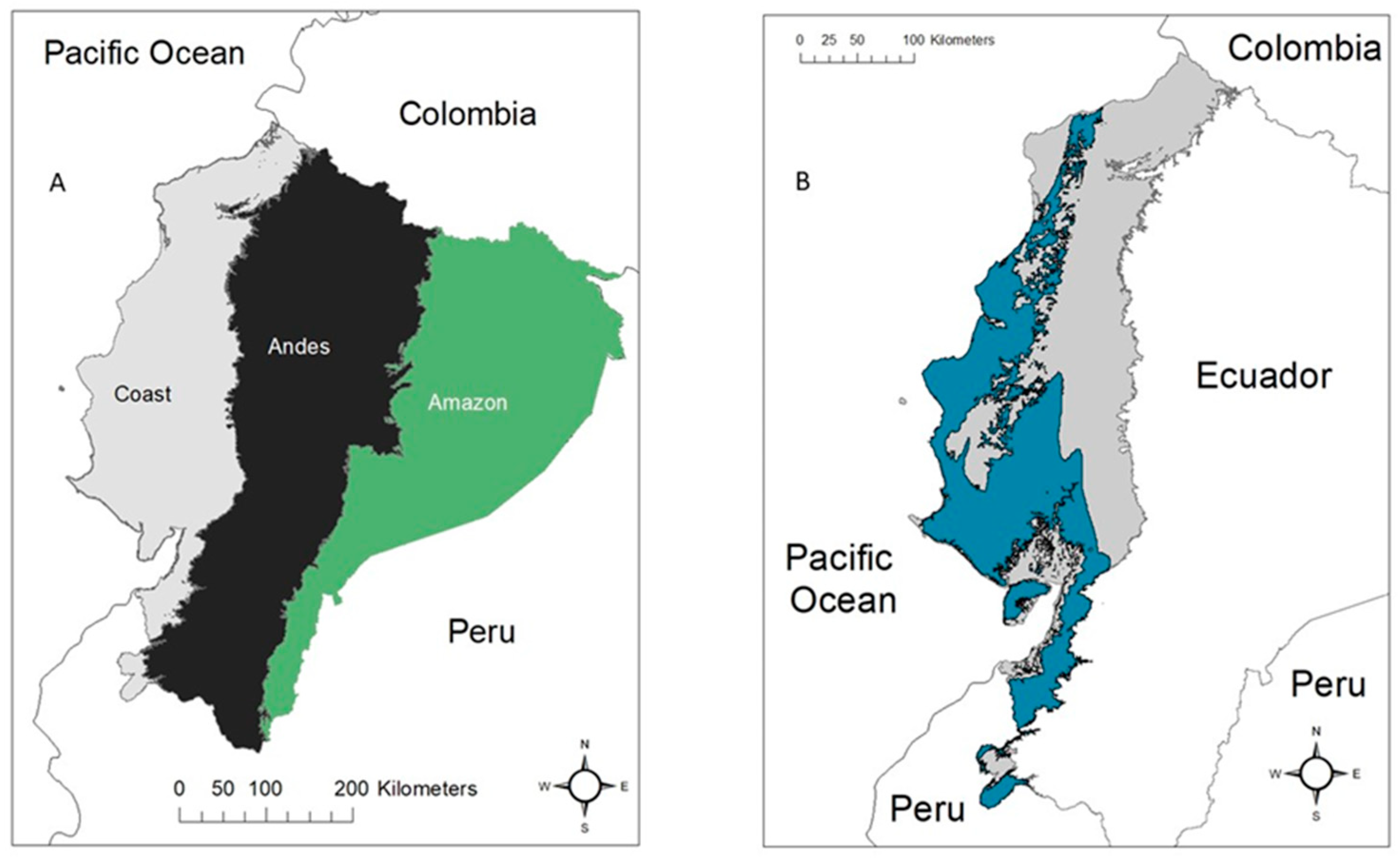
2.1. Study Area
2.2. Dry Forest Characterization
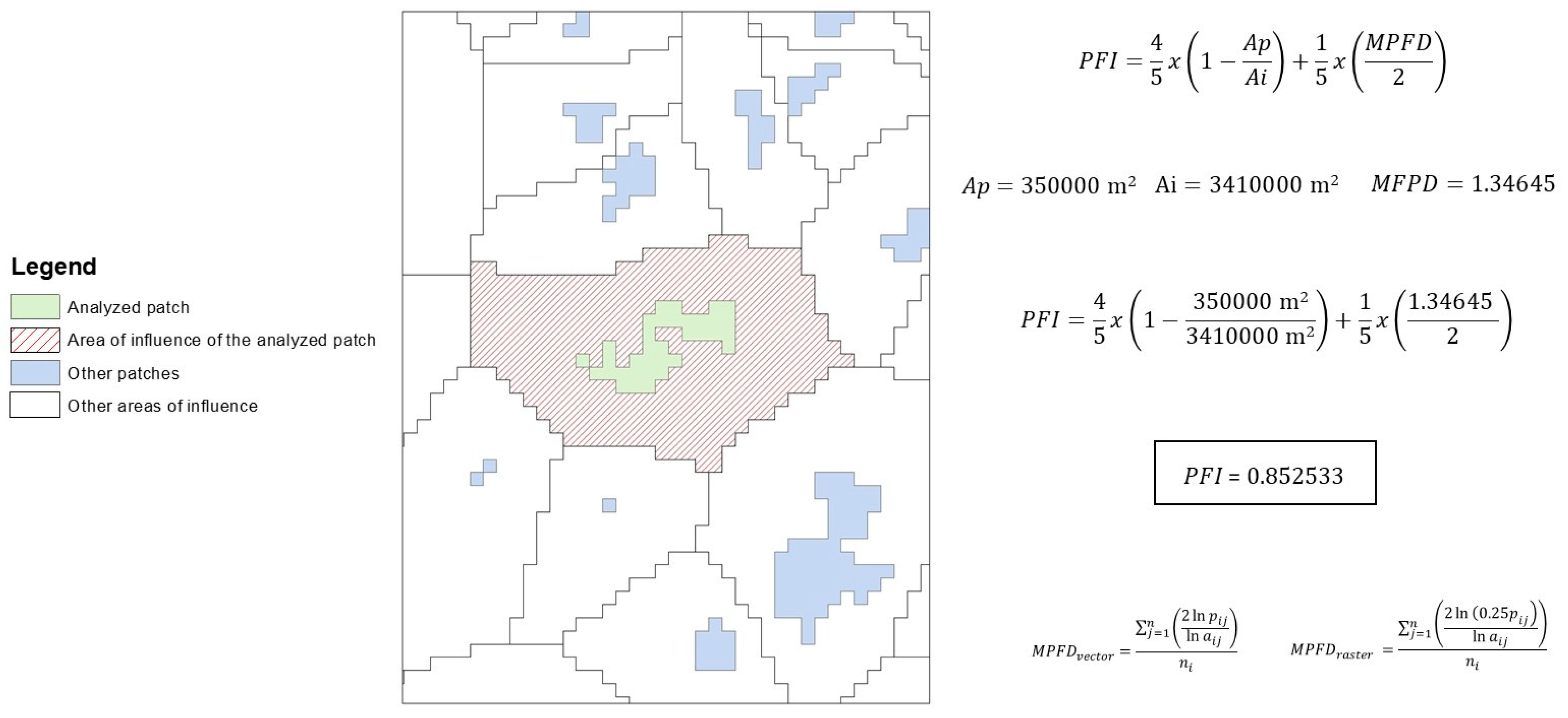
2.3. Fragmentation Metrics
2.4. Temporal Change in Fragmentation Based on PFI with Hexagon Grid and Areas of Influence
2.5. Fragmentation Spatial Patterns
3. Results
3.1. Fragmentation Metrics
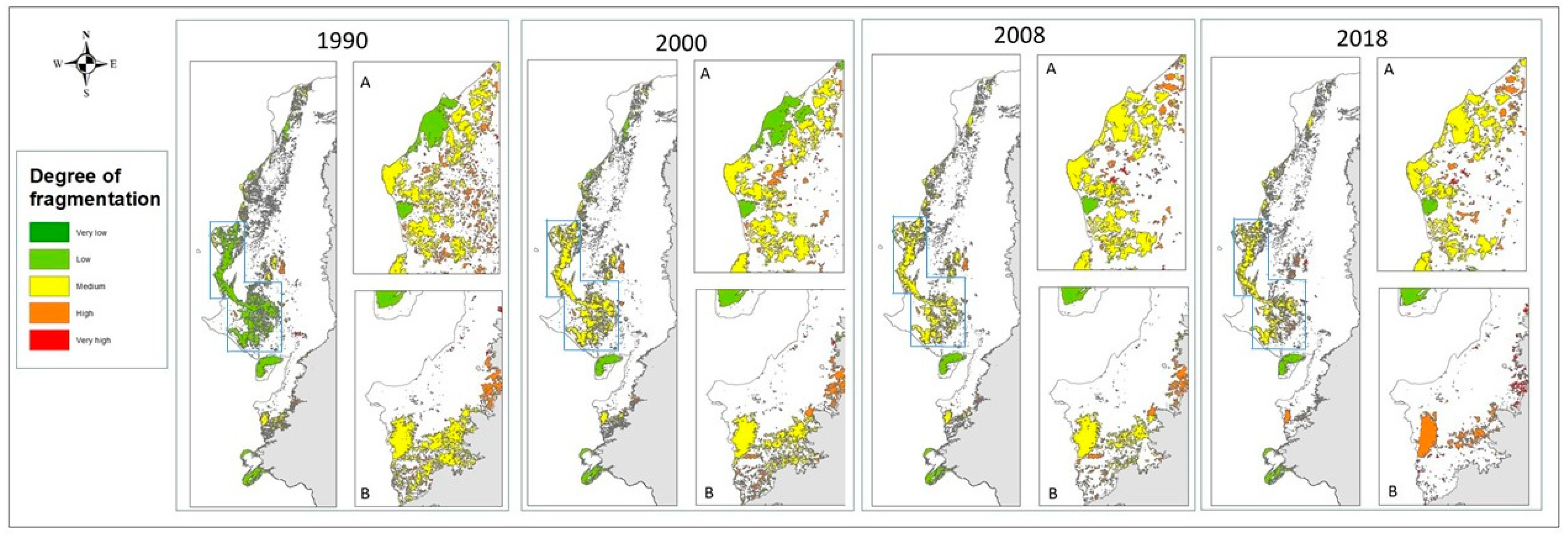
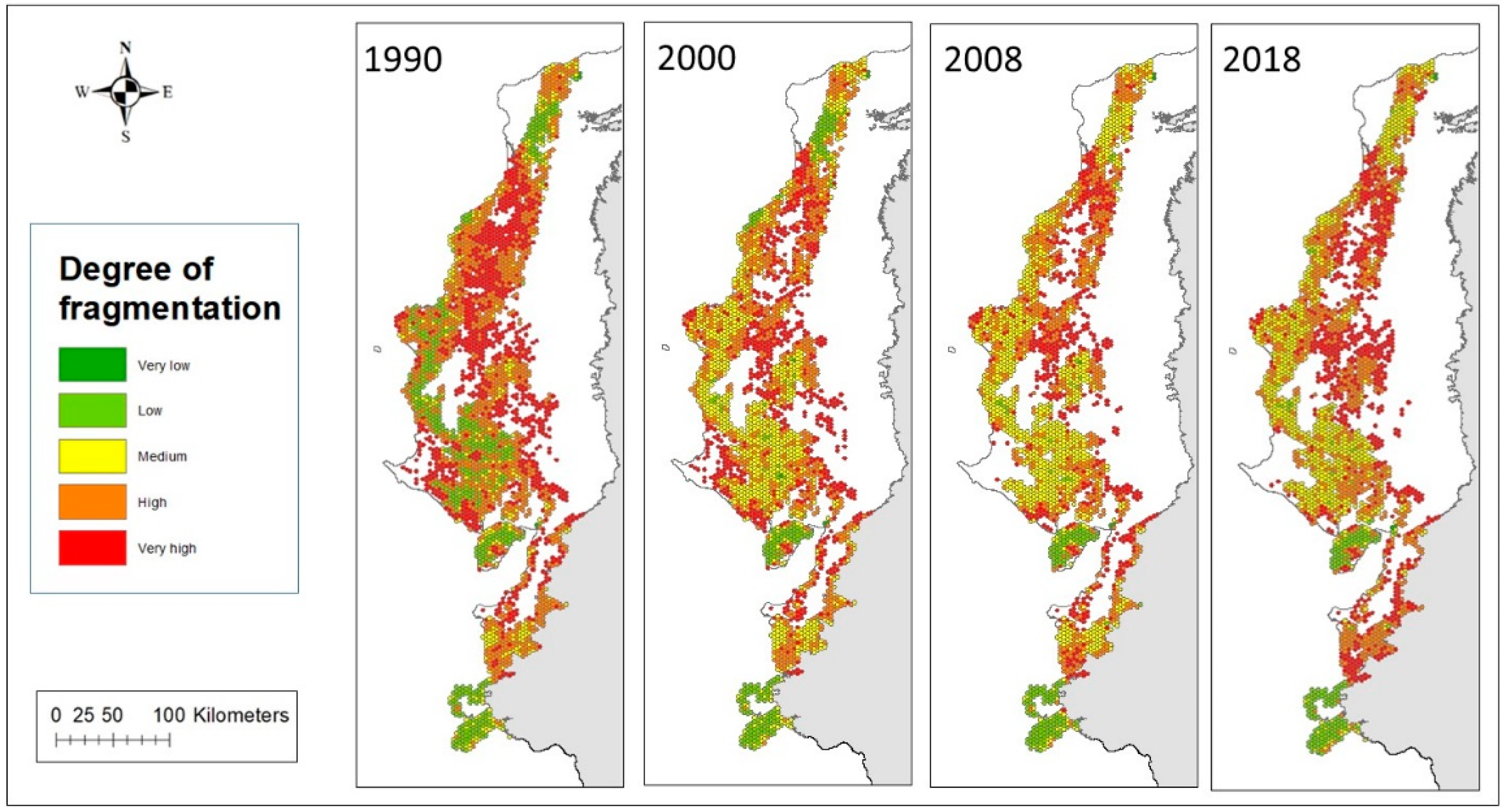
3.2. Temporal Change in Fragmentation Based on PFI with Hexagon Grid and Areas of Influence
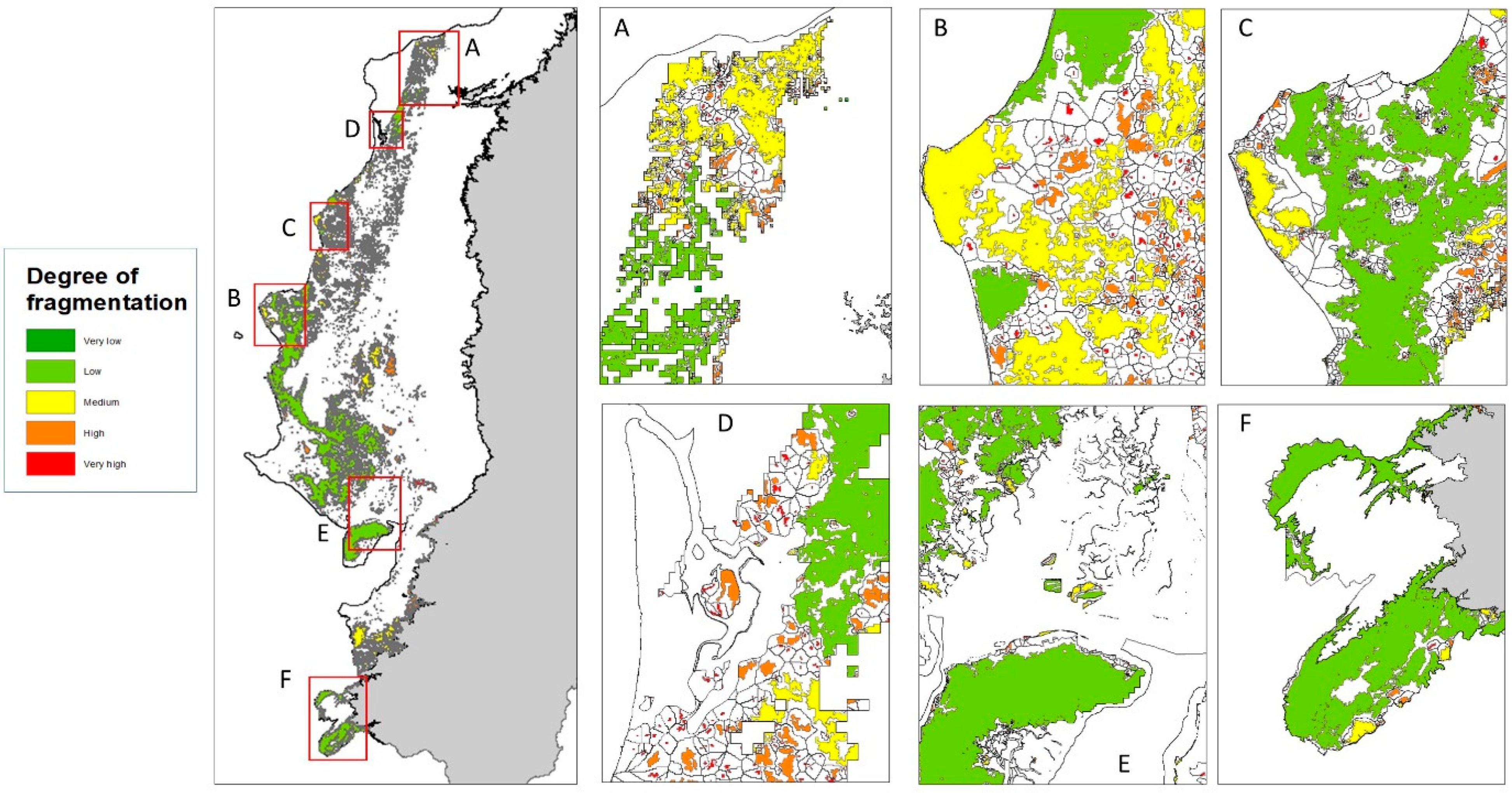
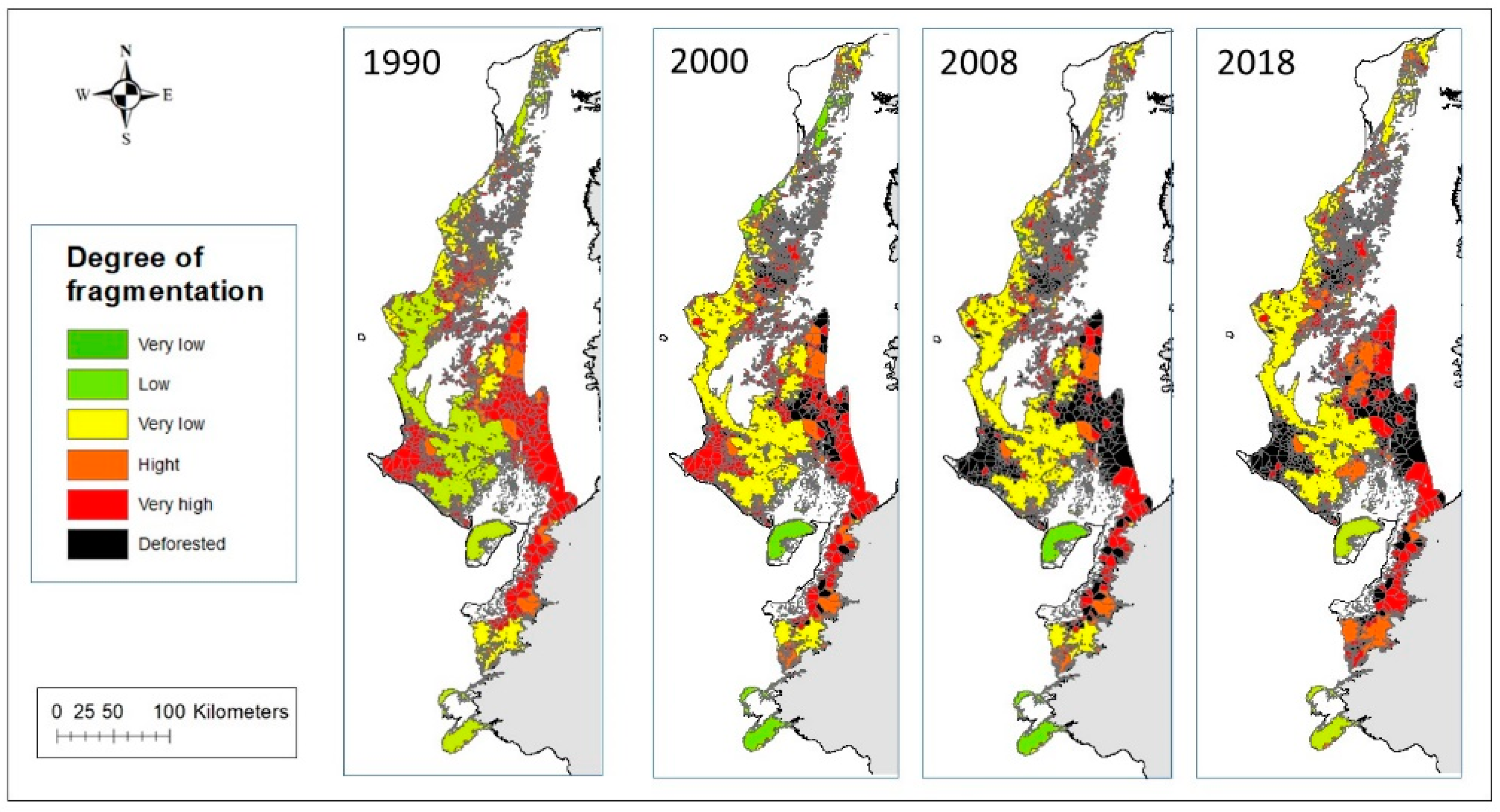
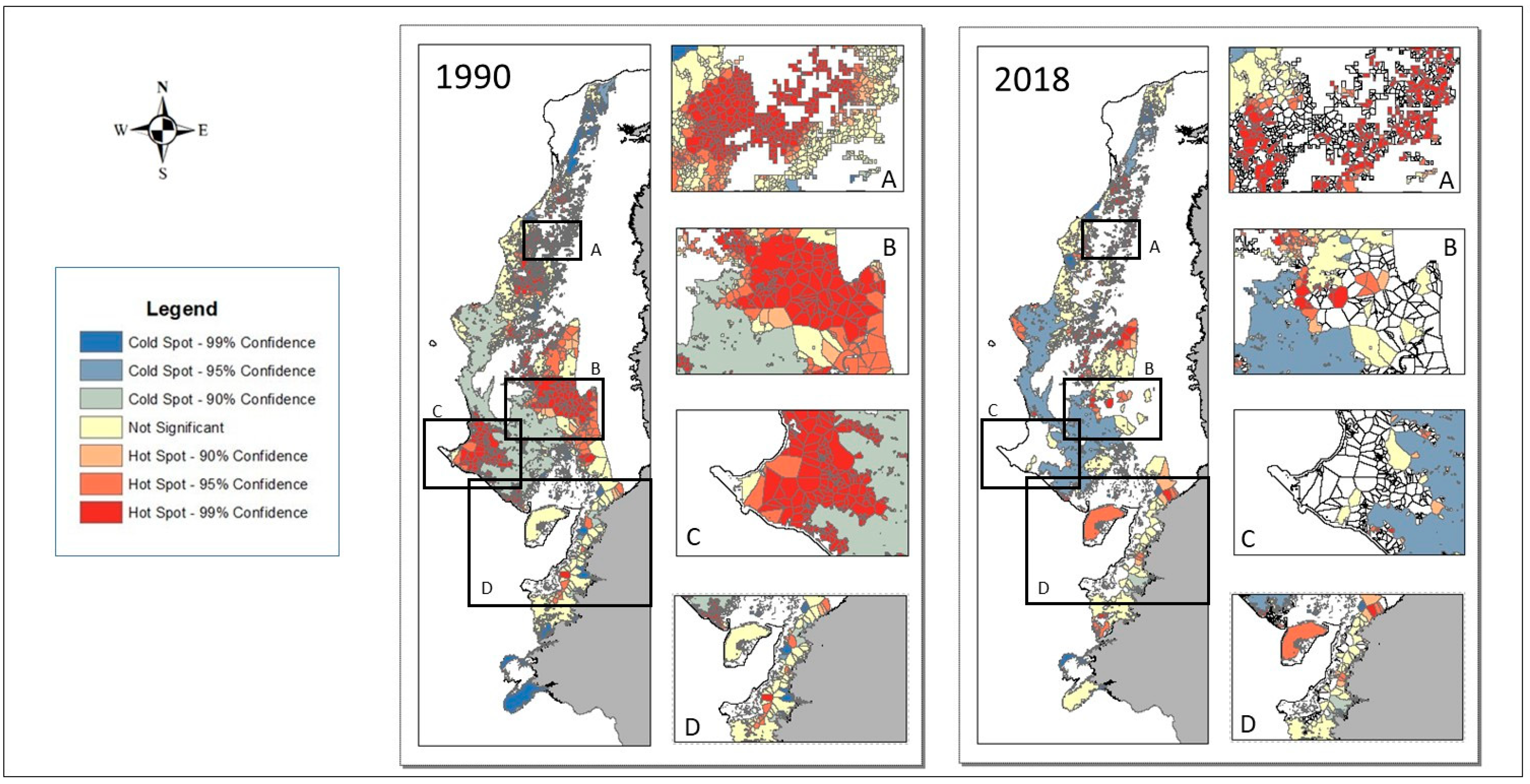
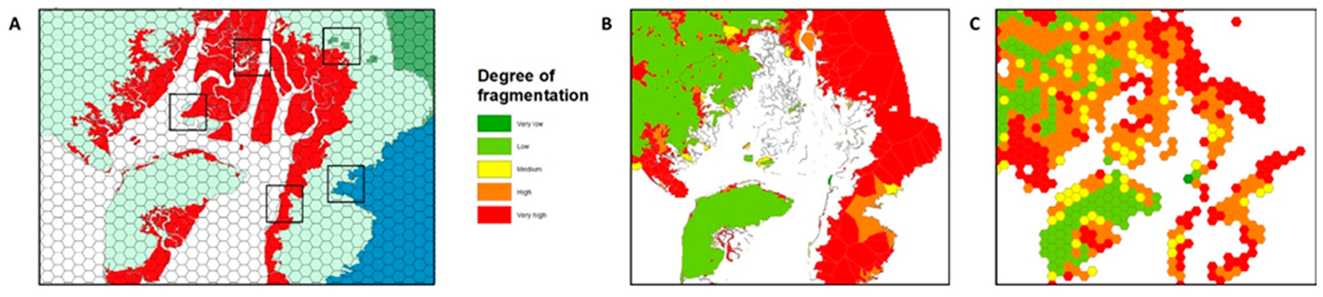
3.3. Fragmentation Spatial Patterns
4. Discussion
4.1. Fragmentation Metrics
4.2. Fragmentation of Seasonal Dry Forest in Ecuador
4.3. Fragmentation Spatial Patterns
5. Conclusions
Author Contributions
Funding
Institutional Review Board Statement
Data Availability Statement
Acknowledgments
Conflicts of Interest
Appendix A
References
- Biodiversity Indicators Partnership. Guidance for National Biodiversity Indicator Development and Use; UNEP World Conservation Monitoring Centre: Cambridge, UK, 2011; 40p. [Google Scholar]
- Parr, T.W.; Jongman, R.H.G.; Külvik, M. Design of a Plan for an Integrated Biodiversity Observing System in Space and Time. The Selection of Biodiversity Indicators for EBONE Development Work; European Biodiversity Observation Network. 2010. Available online: https://nora.nerc.ac.uk/id/eprint/9585/1/EBONE_D1-1_Indicators_Feb10-V2-11-final.pdf (accessed on 10 October 2022).
- 2010 Biodiversity Indicators Partnership. Biodiversity Indicators and the 2010 Target: Outputs, Experiences and Lessons Learnt from the 2010 Biodiversity Indicators Partnership; Secretariat of the Convention on Biological Diversity: Montréal, QC, Canada, 2010; ISBN 9292252720.
- Arasa-Gisbert, R.; Arroyo-Rodríguez, V.; Andresen, E. El Debate Sobre Los Efectos de La Fragmentación Del Hábitat: Causas y Consecuencias. Ecosistemas 2021, 30, 3. [Google Scholar] [CrossRef]
- Carranza, M.L.; Hoyos, L.; Frate, L.; Acosta, A.T.R.; Cabido, M. Measuring Forest Fragmentation Using Multitemporal Forest Cover Maps: Forest Loss and Spatial Pattern Analysis in the Gran Chaco, Central Argentina. Landsc. Urban Plan. 2015, 143, 238–247. [Google Scholar] [CrossRef]
- Fahrig, L.; Arroyo-Rodríguez, V.; Bennett, J.R.; Boucher-Lalonde, V.; Cazetta, E.; Currie, D.J.; Eigenbrod, F.; Ford, A.T.; Harrison, S.P.; Jaeger, J.A.G.; et al. Is Habitat Fragmentation Bad for Biodiversity? Biol. Conserv. 2019, 230, 179–186. [Google Scholar] [CrossRef] [Green Version]
- Kupfer, J.A. National Assessments of Forest Fragmentation in the US. Glob. Environ. Chang. 2006, 16, 73–82. [Google Scholar] [CrossRef]
- Rogan, J.E.; Lacher, T.E. Impacts of Habitat Loss and Fragmentation on Terrestrial Biodiversity; Elsevier Inc.: Amsterdam, The Netherlands, 2018; ISBN 9780124095489. [Google Scholar]
- Trejo, I.; Dirzo, R. Deforestation of Seasonally Dry Tropical Forest: A National and Local Analysis in Mexico. Biol. Conserv. 2000, 94, 133–142. [Google Scholar] [CrossRef]
- Laurance, W.F.; Carolina Useche, D.; Rendeiro, J.; Kalka, M.; Bradshaw, C.J.A.; Sloan, S.P.; Laurance, S.G.; Campbell, M.; Abernethy, K.; Alvarez, P.; et al. Averting Biodiversity Collapse in Tropical Forest Protected Areas. Nature 2012, 489, 290–293. [Google Scholar] [CrossRef] [Green Version]
- Ramírez-Delgado, J.P.; Di Marco, M.; Watson, J.E.M.; Johnson, C.J.; Rondinini, C.; Corredor Llano, X.; Arias, M.; Venter, O. Matrix Condition Mediates the Effects of Habitat Fragmentation on Species Extinction Risk. Nat. Commun. 2022, 13, 595. [Google Scholar] [CrossRef]
- Teixido, A.L.; Gonçalves, S.R.A.; Fernández-Arellano, G.J.; Dáttilo, W.; Izzo, T.J.; Layme, V.M.G.; Moreira, L.F.B.; Quintanilla, L.G. Major Biases and Knowledge Gaps on Fragmentation Research in Brazil: Implications for Conservation. Biol. Conserv. 2020, 251, 108749. [Google Scholar] [CrossRef]
- Fardila, D.; Kelly, L.T.; Moore, J.L.; McCarthy, M.A. A Systematic Review Reveals Changes in Where and How We Have Studied Habitat Loss and Fragmentation over 20 Years. Biol. Conserv. 2017, 212, 130–138. [Google Scholar] [CrossRef]
- Hermosilla, T.; Wulder, M.A.; White, J.C.; Coops, N.C.; Pickell, P.D.; Bolton, D.K. Impact of Time on Interpretations of Forest Fragmentation: Three-Decades of Fragmentation Dynamics over Canada. Remote Sens. Environ. 2018, 222, 65–77. [Google Scholar] [CrossRef]
- Dener, E.; Ovadia, O.; Shemesh, H.; Altman, A.; Chen, S.C.; Giladi, I. Direct and Indirect Effects of Fragmentation on Seed Dispersal Traits in a Fragmented Agricultural Landscape. Agric. Ecosyst. Environ. 2021, 309, 107273. [Google Scholar] [CrossRef]
- Asbjornsen, H.; Ashton, M.S.; Vogt, D.J.; Palacios, S. Effects of Habitat Fragmentation on the Buffering Capacity of Edge Environments in a Seasonally Dry Tropical Oak Forest Ecosystem in Oaxaca, Mexico. Agric. Ecosyst. Environ. 2004, 103, 481–495. [Google Scholar] [CrossRef]
- Tapia-Armijos, M.F.; Homeier, J.; Espinosa, C.I.; Leuschner, C.; De La Cruz, M. Deforestation and Forest Fragmentation in South Ecuador since the 1970s-Losing a Hotspot of Biodiversity. PLoS ONE 2015, 10, e0133701. [Google Scholar] [CrossRef] [Green Version]
- Ries, L.; Fletcher, R.J.; Battin, J.; Sisk, T.D. Ecological Responses to Habitat Edges: Mechanisms, Models, and Variability Explained. Annu. Rev. Ecol. Evol. Syst. 2004, 35, 491–522. [Google Scholar] [CrossRef] [Green Version]
- Chakraborty, A.; Ghosh, A.; Sachdeva, K.; Joshi, P.K. Characterizing Fragmentation Trends of the Himalayan Forests in the Kumaon Region of Uttarakhand, India. Ecol. Inform. 2017, 38, 95–109. [Google Scholar] [CrossRef]
- Fahrig, L. Effects of Habitat Fragmentation on Biodiversity. Annu. Rev. Ecol. Evol. Syst. 2003, 34, 487–515. [Google Scholar] [CrossRef] [Green Version]
- Didham, R.K.; Kapos, V.; Ewers, R.M. Rethinking the Conceptual Foundations of Habitat Fragmentation Research. Oikos 2012, 121, 161–170. [Google Scholar] [CrossRef]
- Fahrig, L. Ecological Responses to Habitat Fragmentation Per Se. Annu. Rev. Ecol. Evol. Syst. 2017, 48, 1–23. [Google Scholar] [CrossRef]
- Fahrig, L. Why Do Several Small Patches Hold More Species than Few Large Patches? Glob. Ecol. Biogeogr. 2020, 29, 615–628. [Google Scholar] [CrossRef] [Green Version]
- Herrera, L.P.; Sabatino, M.C.; Jaimes, F.R.; Saura, S. Landscape Connectivity and the Role of Small Habitat Patches as Stepping Stones: An Assessment of the Grassland Biome in South America. Biodivers. Conserv. 2017, 26, 3465–3479. [Google Scholar] [CrossRef]
- Wintle, B.A.; Kujala, H.; Whitehead, A.; Cameron, A.; Veloz, S.; Kukkala, A.; Moilanen, A.; Gordon, A.; Lentini, P.E.; Cadenhead, N.C.R.; et al. Global Synthesis of Conservation Studies Reveals the Importance of Small Habitat Patches for Biodiversity. Proc. Natl. Acad. Sci. USA 2019, 116, 909–914. [Google Scholar] [CrossRef] [Green Version]
- Tulloch, A.I.T.; Barnes, M.D.; Ringma, J.; Fuller, R.A.; Watson, J.E.M. Understanding the Importance of Small Patches of Habitat for Conservation. J. Appl. Ecol. 2016, 53, 418–429. [Google Scholar] [CrossRef] [Green Version]
- Jackson, H.B.; Fahrig, L. Habitat Loss and Fragmentation. In Encyclopedia of Biodiversity; Scheiner, S.M., Ed.; Elsevier: Amsterdam, The Netherlands, 2013; Volume 4, pp. 50–58. ISBN 9780123847195. [Google Scholar]
- Rios, E.; Benchimol, M.; Dodonov, P.; De Vleeschouwer, K.; Cazetta, E. Testing the Habitat Amount Hypothesis and Fragmentation Effects for Medium- and Large-Sized Mammals in a Biodiversity Hotspot. Landsc. Ecol. 2021, 36, 1311–1323. [Google Scholar] [CrossRef]
- Fletcher, R.J.; Didham, R.K.; Banks-Leite, C.; Barlow, J.; Ewers, R.M.; Rosindell, J.; Holt, R.D.; Gonzalez, A.; Pardini, R.; Damschen, E.I.; et al. Is Habitat Fragmentation Good for Biodiversity? Biol. Conserv. 2018, 226, 9–15. [Google Scholar] [CrossRef] [Green Version]
- Fahrig, L. Habitat Fragmentation: A Long and Tangled Tale. Glob. Ecol. Biogeogr. 2019, 28, 33–41. [Google Scholar] [CrossRef]
- McGarigal, K.; Marks, B. FRAGSTATS: Spatial Pattern Analysis Program for Quantifying Landscape Structure. 1994. Available online: http://www.edc.uri.edu/nrs/classes/nrs534/fragstats.pdf (accessed on 10 October 2022).
- Bestion, E.; Cote, J.; Jacob, S.; Winandy, L.; Legrand, D. Habitat Fragmentation Experiments on Arthropods: What to Do Next? Curr. Opin. Insect Sci. 2019, 35, 117–122. [Google Scholar] [CrossRef] [Green Version]
- Hargis, C.D.; Bissonette, J.A.; David, J.L. The Behavior of Landscape Metrics Commonly Used in the Study of Habitat Fragmentation. Landsc. Ecol. 1998, 13, 167–186. [Google Scholar] [CrossRef]
- Myers, N.; Mittermeier, R.A.; Mittermeier, C.G.; da Fonseca, G.A.B.; Kent, J. Biodiversity Hotspots for Conservation Priorities. Nature 2000, 403, 853–858. [Google Scholar] [CrossRef]
- Rivas, C.A.; Guerrero-casado, J.; Navarro-cerillo, R.M. Deforestation and Fragmentation Trends of Seasonal Dry Tropical Forest in Ecuador: Impact on Conservation. For. Ecosyst. 2021, 8, 46. [Google Scholar] [CrossRef]
- Rivas, C.A.; Navarro-Cerillo, R.M.; Johnston, J.C.; Guerrero-Casado, J. Dry Forest Is More Threatened but Less Protected than Evergreen Forest in Ecuador’s Coastal Region. Environ. Conserv. 2020, 47, 79–83. [Google Scholar] [CrossRef]
- Prentice, K.C. Bioclimatic Distribution of Vegetation for General Circulation Model Studies. J. Geophys. Res. 1990, 95, 11811–11830. [Google Scholar] [CrossRef]
- Ministerio del ambiente del Ecuador. Sistema de Clasificación de Los Ecosistemas Del Ecuador Continental; Subsecretaría de Patrimonio Natural: Quito, Ecuador, 2013; ISBN 9786077629016.
- Ministerio del Ambiente Fenologia. Available online: http://qa-ide.ambiente.gob.ec:8080/geonetwork/srv/api/records/64f61941-168c-4f4f-837b-5a3172c26d8e022 (accessed on 10 October 2022).
- Ministerio del Ambiente Regimen de Inundacion. Available online: http://qa-ide.ambiente.gob.ec:8080/geonetwork/srv/api/records/64f61941-168c-4f4f-837b-5a3172c26d8e041/formatters/xsl-view?view=inspire&portalLink= (accessed on 10 October 2022).
- Ministerio del Ambiente Bioclima. Available online: http://qa-ide.ambiente.gob.ec:8080/geonetwork/srv/api/records/64f61941-168c-4f4f-837b-5a3172c26d8e039 (accessed on 10 October 2022).
- Peralvo, M.; Delgado, J. Metodología Para La Generación Del Mapa de Deforestación Histórica; Ministerio del Ambiente and CONDESAN: Quito, Ecuador, 2010.
- Ministerio del Ambiente. Línea Base de Deforestación Del Ecuador Continental; Ministerio del Ambiente: Quito, Ecuador, 2012.
- MAE; MAGAP. Protocolo Metodológico Para La Elaboración Del Mapa de Cobertura y Uso de La Tierra Del Ecuador Continental 2013-2014 Escala 1:100.000; Ministerio del Ambiente del Ecuador y Ministerio de Agricultura, Ganadería, Acuacultura y Pesca: Quito, Ecuador, 2015.
- McGarigal, K.; Marks, B.J. FRAGSTATS: Spatial Pattern Analysis Program for Quantifying Landscape Structure; General Technical Report (GTR) PNW-GTR-351; Department of Agriculture, Forest Service, Pacific Northwest Research Station: Portland, OR, USA, 1995.
- Foltête, J.C.; Clauzel, C.; Vuidel, G. A Software Tool Dedicated to the Modelling of Landscape Networks. Environ. Model. Softw. 2012, 38, 316–327. [Google Scholar] [CrossRef]
- Ord, J.K.; Getis, A. Local Spatial Autocorrelation Statistics: Distributional Issues and an Application. Geogr. Anal. 1995, 27, 286–306. [Google Scholar] [CrossRef]
- Feng, Y.; Chen, X.; Gao, F.; Liu, Y. Impacts of Changing Scale on Getis-Ord Gi* Hotspots of CPUE: A Case Study of the Neon Flying Squid (Ommastrephes Bartramii) in the Northwest Pacific Ocean. Acta Oceanol. Sin. 2018, 37, 67–76. [Google Scholar] [CrossRef]
- Riitters, K.H.; O’Neill, R.V.; Hunsaker, C.T.; Wickham, J.D.; Yankee, D.H.; Timmins, S.P.; Jones, K.B.; Jackson, B.L. A Factor Analysis of Landscape Pattern and Structure Metrics. Landsc. Ecol. 1995, 10, 23–39. [Google Scholar] [CrossRef]
- Cushman, S.A.; McGarigal, K.; Neel, M.C. Parsimony in Landscape Metrics: Strength, Universality, and Consistency. Ecol. Indic. 2008, 8, 691–703. [Google Scholar] [CrossRef]
- Chen, A.; Yao, L.; Sun, R.; Chen, L. How Many Metrics Are Required to Identify the Effects of the Landscape Pattern on Land Surface Temperature? Ecol. Indic. 2014, 45, 424–433. [Google Scholar] [CrossRef]
- Hanski, I.; Gaggiotii, O.E. Ecology, Genetics and Evolution of Metapopulations; Crumly, C.M., Ed.; Elsevier Inc.: Phoenix, AZ, USA, 2004; ISBN 0-12-323448-4. [Google Scholar]
- Ewers, R.M.; Thorpe, S.; Didham, R.K. Synergistic Interactions between Edge and Area Effects in a Heavily Fragmented Landscape. Ecology 2007, 88, 96–106. [Google Scholar] [CrossRef]
- Collinge, S.K. Ecological Consequences of Habitat Fragmentation: Implications for Landscape Architecture and Planning. Landsc. Urban Plan. 1996, 36, 59–77. [Google Scholar] [CrossRef]
- Haddad, N.M.; Brudvig, L.A.; Clobert, J.; Davies, K.F.; Gonzalez, A.; Holt, R.D.; Lovejoy, T.E.; Sexton, J.O.; Austin, M.P.; Collins, C.D.; et al. Habitat Fragmentation and Its Lasting Impact on Earth’s Ecosystems. Sci. Adv. 2015, 1, e1500052. [Google Scholar] [CrossRef]
- Hilty, J.; Worboys, G.L.; Keeley, A.; Woodley, S.; Lausche, B.J.; Locke, H.; Carr, M.; Pulsford, I.; Pittock, J.; White, J.W.; et al. Guidelines for Conserving Connectivity through Ecological Networks and Corridors; IUCN: Gland, Switzerland, 2020. [Google Scholar]
- Smith, V.; Portillo-Quintero, C.; Sanchez-Azofeifa, A.; Hernandez-Stefanoni, J.L. Assessing the Accuracy of Detected Breaks in Landsat Time Series as Predictors of Small Scale Deforestation in Tropical Dry Forests of Mexico and Costa Rica. Remote Sens. Environ. 2019, 221, 707–721. [Google Scholar] [CrossRef]
- Ministerio del ambiente de Ecuador. Fragmentacion De Ecosistemas Del Ecuador Contimental; Subsecretaria de Patrimonio Natural: Quito, Ecuador, 2015.
- Birch, C.P.D.; Oom, S.P.; Beecham, J.A. Rectangular and Hexagonal Grids Used for Observation, Experiment and Simulation in Ecology. Ecol. Modell. 2007, 206, 347–359. [Google Scholar] [CrossRef]
- Law, E.A.; Bryan, B.A.; Meijaard, E.; Mallawaarachchi, T.; Struebig, M.; Wilson, K.A. Ecosystem Services from a Degraded Peatland of Central Kalimantan: Implications for Policy, Planning, and Management. Ecol. Appl. 2015, 25, 70–87. [Google Scholar] [CrossRef]
- Rabe, S.E.; Koellner, T.; Marzelli, S.; Schumacher, P.; Grêt-Regamey, A. National Ecosystem Services Mapping at Multiple Scales-The German Exemplar. Ecol. Indic. 2016, 70, 357–372. [Google Scholar] [CrossRef]
- Rodríguez, N.; Armenteras, D.; Retana, J. National Ecosystems Services Priorities for Planning Carbon and Water Resource Management in Colombia. Land Use Policy 2015, 42, 609–618. [Google Scholar] [CrossRef]


| Descriptive Statistics | Year | |||
|---|---|---|---|---|
| 1990 | 2000 | 2008 | 2018 | |
| N°. deforested patches | 0 | 2481 | 3348 | 3451 |
| Mean | 0.81 | 0.85 | 0.87 | 0.88 |
| Median | 0.85 | 0.90 | 0.92 | 0.99 |
| S.D | 0.09 | 0.13 | 0.13 | 0.12 |
| Year | 1990 | 2000 | 2008 | 2018 |
|---|---|---|---|---|
| N°. of hexagons | 3091 | 2919 | 2681 | 2741 |
| Mean | 0.67 | 0.63 | 0.62 | 0.66 |
| Median | 0.73 | 0.65 | 0.63 | 0.69 |
| S.D | 0.16 | 0.17 | 0.15 | 0.15 |
| 2018 | ||||||
|---|---|---|---|---|---|---|
| Cold | NS | Hot | Deforested | Total | ||
| 1990 | Cold | 879 | 314 | 22 | 505 | 1720 |
| NS | 139 | 634 | 403 | 1138 | 2314 | |
| Hot | 19 | 228 | 819 | 1808 | 2874 | |
| Total | 1037 | 1176 | 1244 | 3451 | 6908 | |
| Metrics | Conclusions and Implications | Problem Description | Graphical Representation | |
|---|---|---|---|---|
| Area | The larger the average area, the less fragmentation. | A | In figure A.1, there is a greater mean area; however, figure A.2 shows less fragmentation. | 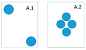 |
| Area/Perimeter | The smaller the area/perimeter, the greater the fragmentation. | B | In figure B.1, there is higher area/perimeter; however, figure B.2 shows higher fragmentation. | 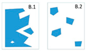 |
| MPFD and other shape parameters. | In more complex forms, there is greater fragmentation. | C | In figure C.1, the patches have more complex shapes; however, figure C.2 shows greater fragmentation. | 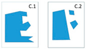 |
| Distance | The shorter the mean distance, the less fragmentation. | D | In figure D.1, the patches have a greater mean distance; however, figure D.2 shows greater fragmentation. | 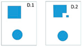 |
| Number of patches | The lower the number of patches, the less fragmentation. | A | In figure A.1, there are fewer patches; however, figure A.2 shows less fragmentation. | 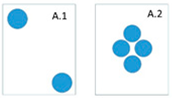 |
| Core Area | Undisturbed areas within the patch—the greater the core area, the less fragmentation. | The core area is based on the species and on the area that the species needs eliminating the edge effect, but it starts from the premise that the edges are detrimental to the species, though this is not always the case. | ||
Publisher’s Note: MDPI stays neutral with regard to jurisdictional claims in published maps and institutional affiliations. |
© 2022 by the authors. Licensee MDPI, Basel, Switzerland. This article is an open access article distributed under the terms and conditions of the Creative Commons Attribution (CC BY) license (https://creativecommons.org/licenses/by/4.0/).
Share and Cite
Rivas, C.A.; Guerrero-Casado, J.; Navarro-Cerrillo, R.M. A New Combined Index to Assess the Fragmentation Status of a Forest Patch Based on Its Size, Shape Complexity, and Isolation. Diversity 2022, 14, 896. https://doi.org/10.3390/d14110896
Rivas CA, Guerrero-Casado J, Navarro-Cerrillo RM. A New Combined Index to Assess the Fragmentation Status of a Forest Patch Based on Its Size, Shape Complexity, and Isolation. Diversity. 2022; 14(11):896. https://doi.org/10.3390/d14110896
Chicago/Turabian StyleRivas, Carlos A., José Guerrero-Casado, and Rafael M. Navarro-Cerrillo. 2022. "A New Combined Index to Assess the Fragmentation Status of a Forest Patch Based on Its Size, Shape Complexity, and Isolation" Diversity 14, no. 11: 896. https://doi.org/10.3390/d14110896