Article

Whole System Data Integration for Condition Assessments of Climate Change Impacts: An Example in High-Mountain Ecosystems in Rila (Bulgaria)

by
Kostadin Katrandzhiev
*,
Kremena Gocheva
and
Svetla Bratanova-Doncheva
Institute of Biodiversity and Ecosystem Research, Bulgarian Academy of Sciences, 2 Yurij Gagarin St., 1113 Sofia, Bulgaria
*
Author to whom correspondence should be addressed.
Diversity 2022, 14(4), 240; https://doi.org/10.3390/d14040240
Submission received: 7 October 2021 / Revised: 16 March 2022 / Accepted: 18 March 2022 / Published: 25 March 2022
(This article belongs to the Special Issue Forest Management and Biodiversity Conservation)

Abstract

:
To study climate impacts, data integration from heterogeneous sources is imperative for long-term monitoring in data sparse areas such as the High Mountain Ecosystems in the Rila Mountain, Bulgaria—difficult to both access and observe remotely due to frequent clouds. This task is especially challenging because discerning trends in vegetation location, condition and functioning requires observing over decades. To integrate the existing sparse data, we apply the Whole System framework adapted nationally in the Bulgarian Methodological Framework for Mapping and Assessment of ecosystem services. As the framework mainly relies on field data, we complement it with remote sensing vegetation indices (NDVI, NDWI and NDGI) for 42 years, together with Copernicus High Resolution Layer products and climate change reanalysis data for 40 years. We confirmed that the Whole System framework is extensible and semantically, ontologically and methodologically well suited for heterogeneous data fusion, co-analysis, reanalysis and joint interpretation. We found trends in ecosystem extent and functioning, in particular species composition, in line with climate change trends since around 1990 and exclusively attributable to climate change since 2015. Furthermore, we specified a data crosswalk between habitats and ecosystems at Level 3 (ecosystem subtype), and define new candidate indicators suitable for remotely monitoring climate change’s effects on the ecosystems’ extent and condition, as candidates for inclusion in the methodological framework.

Graphical Abstract

1. Introduction

The ecologically complex high mountain ecosystems (HMEs) are important study areas for climate change impact on ecosystem structure and functions. There is a wide range of concepts about ecosystem functioning, reviewed by Pettorelli et al. (2017) [1].
Scientists studying HMEs attempt to explain the influence of climate change on the vegetation structure [2,3], causation processes [4], spatial distribution in HMEs [5,6,7] and the adaptive capacity of HMEs to the influence of natural and/or anthropogenic changes [8]. In doing so, they invariably come across the overwhelming complexity of the interrelated study objects of HMEs and climate change.
As a means to reduce complexity, research often focuses on specific aspects such as the ecotone rather than the entire ecosystem [5,9,10,11,12,13,14,15], abiotic factors [16], species composition and dynamics [17,18]. However, a truly holistic assessment of both condition and functioning trends for these highly sensitive and vulnerable zones in their entirety requires an integrated interdisciplinary approach. Different types of data are collected at different points in time and space, different scale, for different purposes and using different—in the cases of remote sensing and climate modelling significantly improved—instruments and methods over time. These objective challenges include:
  • Combining continuous and discrete data. Verifying ecosystem type typically relates to one-off observations of ground data; remote sensing imagery is continuous in space but discrete in time, while climate models have spatial and temporal continuity;
  • Data heterogeneity. Even within the same ecosystem, the scope, field measurement methods and even the underlying indicators, classifications and other conceptual elements may vary significantly, making the results difficult to reconcile and reuse. Climate models render differently accurate results and are periodically corrected through reanalysis, resulting in different variables for the new data series;
  • Data imbalances—biases in the scientific and management interest with data collection (predominantly about the forest ecosystem), and technological imbalances due to the different quality of remote sensing equipment over time and the increasing number of missions in the last years. As a result, there is a much better availability and quality of remote sensing scenes in the last five years than at any time before, and this development is accelerating;
  • In addition to the usual difficulties of data integration listed above, the study of HMEs meets specific difficulties that lead to a data scarcity:
    HMEs are often difficult to access physically for surveys, species inventories or installing/maintaining monitoring equipment for long-term observations;
    Automated measurements meet the challenges of weak or lacking internet connectivity and natural hazards such as avalanches that damage or annihilate the equipment;
    During the vegetation season HMEs in good condition act as a biotic pump that increases air humidity [19,20] and hence their remote sensing often reveals clouds. Even where there are no visible clouds, there often are variable patterns of mist or fog [21,22] that may remain undetected in cloud masking. These atmospheric conditions distort the sensor readings and cause errors in the values of vegetation indices; their precise detection typically requires another data source, i.e., ground data validation or accurate meteorological data. This makes remote phenological observations virtually unfeasible;
    Scale discrepancies: Microclimatic influences largely shape developments on the ground, while climate models such as ECMWF Re-Analysis (ERA) we use in this study are much coarser. Satellite imagery is constantly improving, with the pixel size reduced by orders of magnitude between early products and current very high-resolution ones, making it commensurate with the size of field sites. Such great differences in scale make data fusion imperative for the use of ERA Interim and future use of ERA 5 together with other available data since no sufficient downscaling is possible in such a discrepant scenario. While ERA Interim uncertainty is relatively low at a large scale for the key parameters relevant to our study (precipitation dry bias of −1% for Europe according to [23], temperature uncertainty of ±2% according to [24]), regional (microclimatic) variation is not captured well due to their coarse granularity [25] and downscaling them is challenging (as evidenced by the modelling effort behind the Vito dataset “Climate variables for cities in Europe from 2008 to 2017” documented at https://cds.climate.copernicus.eu/cdsapp#!/dataset/sis-urban-climate-cities?tab=overview (accessed on 17 March 2022) which is not maintained beyond the contract and did not manage significant downscaling even in areas with a high density of meteorological observation points). This great difference in scales of datasets is the reason to consider climate models only for exploring HMEs qualitatively at this stage, as they are far from sufficiently detailed at the scales commensurate with most monitoring needs. Their use remains indispensable despite the large scale since they are the only available approximation of weather information in data poor areas.
    Finally yet importantly, protected areas containing HMEs are not so interesting commercially which exacerbates the bias of data collection and monitoring towards inhabited or managed territories such as cities or agricultural areas.
Despite these challenges, complex assessments mandate going beyond the sole use of field observation methods that mainly inform on ecosystem structure, not functions [1]. This is especially true for Bulgaria where field observations are still the preferred method of ecosystem research (also reflected in the parameter measurement methods in [26]). Climate models are increasingly accessible and precise, and the verification in different regions shows their suitability for observing trends even in the presence of biases in some parameters [27]. They therefore provide useful guidelines on climate change over longer periods in areas with no direct observations available. Remote sensing methods are applicable to ecosystem monitoring [28] and widely used for landscape (ecosystem) change detection and land cover classification, monitoring condition and functioning trends and disturbance factors [29], changes in growth conditions, growing season length, shifts in vegetation [30] and natural capital accounting [31,32]. The latest observations benefit from the improved data quality due to the technological (sensor) innovation in the past decades and increasingly allow for observing ecosystem services [33].
Combining data from sources as diverse as field surveys, remote sensing and constrained climate reanalysis models bring their own set of technological and cognitive challenges. Different data require different sets of expertise to process and analyze. No single researcher is equally proficient in all these methods and structuring teamwork for interdisciplinary data integration requires each member of the interdisciplinary team to be sufficiently aware of all data and the processing steps everyone else performs on it. Therefore, the optimal and efficient reuse of the efforts of large teams in producing assessments and models on the national or continental scale becomes essential for smaller research teams. Data processing disciplines like ecoinformatics [34] rely upon solutions that follow the Findable, Accessible, Interoperable and Reusable (FAIR) data principles [35] and use standardized technology [36,37,38,39]. However, attempting to bridge the data silos between research disciplines for interdisciplinary ecosystem research meet their cognitive limits, as abundantly discussed by Villa et al. [40] who note the domain dependence of any formalized system of terms and their relations (ontology). Each scientific discipline has its own semantic structure, data and metadata collection models, and nomenclatures and indicator systems (a few examples: (1) Mapping ecosystem to habitat types is a difficult task which becomes ambiguous if such mapping is sought across climatic zones; (2) taxonomical standards for Animalia and Plantae obey similar but not identical principles; (3) the way anthropogenic pressures are described varies between the Driver-Pressure-State-Impact-Response framework (DPSIR) and the reporting guidelines to the EU Habitats Directive; (4) even the same indicator such as biomass may be observed differently depending on the ecosystem type, e.g., using NDVI for terrestrial ecosystems and Chlorophyll A for water bodies, and intercalibrating such different methods to obtain comparable results may be very difficult); some researchers argue that assumptions not contained in the sematic annotation (priors, as termed by Chollet [41]) will always implicitly influence such semantic structures and models. At the end, due to the very diverse and complex nature of their research object, ecosystem researchers have the task to unify conceptual bases in a convergent manner as a mean to integrate the corresponding data initially collected for other purposes (divergent exploration [42]).
In effect, not resolving these issues prevents researchers from efficiently analyzing all available data. Therefore, our first hypothesis is based on the assumption that, by design, a unifying conceptual framework at the ecosystem scale allows for data integration that
(1)
is more ecologically meaningful,
(2)
is more reliable,
(3)
is extensible in terms of indicators and methods, especially in cases of sparse and biased data which can significantly reduce the accuracy of many automated approaches such as machine learning; and
(4)
allows for using all available data from multiple sources across space and time to the extent possible.
In the context of this hypothesis, ecologically meaningful data integration refers to the explainability, through known ecological processes, of data with different types and provenances measured/modelled either at the same time or within ecologically meaningful time intervals. For example, change trends in climate parameters (such as temperature and precipitation) modeled over time, if correlating with field data indicating change of species composition, are consistent with the ecologically meaningful process of upward shift of deciduous species in coniferous forests. Similarly, climate change datasets together with remote sensing data on changing ecosystem extent in the absence of land management are consistent with succession. Of course, having a single ecologically meaningful hypothesis consistent with the data is seldom the case, and in practice it is often necessary to estimate the influence of different co-occurring natural or anthropogenic environmental factors to avoid double counting [43,44]. More reliable data integration refers to the formulation within the same conceptual framework of reproducible new indicators for new policy or research purposes [45]. Such extension must by necessity be founded on the use of different data sources to crosscheck data and exclude incorrect data instances and outliers. Extensible data integration refers to integration methods that allow for adding more data, updating data to perform reanalysis, upscaling or downscaling of data or other necessary changes in the types and properties of data used in the analysis, while at the same time preserving the ecologically meaningful interpretation. To test this hypothesis, in this study we apply the Whole System approach [46,47] as adapted in the Methodological Framework for assessment and mapping of ecosystem condition and ecosystem services in Bulgaria [26], and use all available heterogeneous data. For more on the framework, see Section 2.2.
To our knowledge, to date no studies have been performed in the Whole System context for the long timeframe of several decades on HMEs in Bulgaria or elsewhere.
Based on earlier work [2,5,7], we formulated a second hypothesis, namely: We expected that the species in our study areas’ HME develop in a changing climate, and assess the response of the HME to changes in climate parameters.
The objective of this study is testing these two closely linked hypotheses—the first pertaining to the general methodological principles of data fusion in the Whole System context, and the second to a specific application concerning studying effects of climate change in a representative ecologically interesting but data poor HME area. Testing the second hypothesis using the framework of the first hypothesis allows for simultaneously testing both the method and the ecological hypothesis at once.
To the extent possible, quantitative evaluation criteria are a focus of this assessment—both measurable changes in ecosystems’ spatial distribution at the landscape level (e.g., succession), and observable ecosystem change parameters such as change in species composition [48,49] traceable over the past decades.

2. Materials and Methods
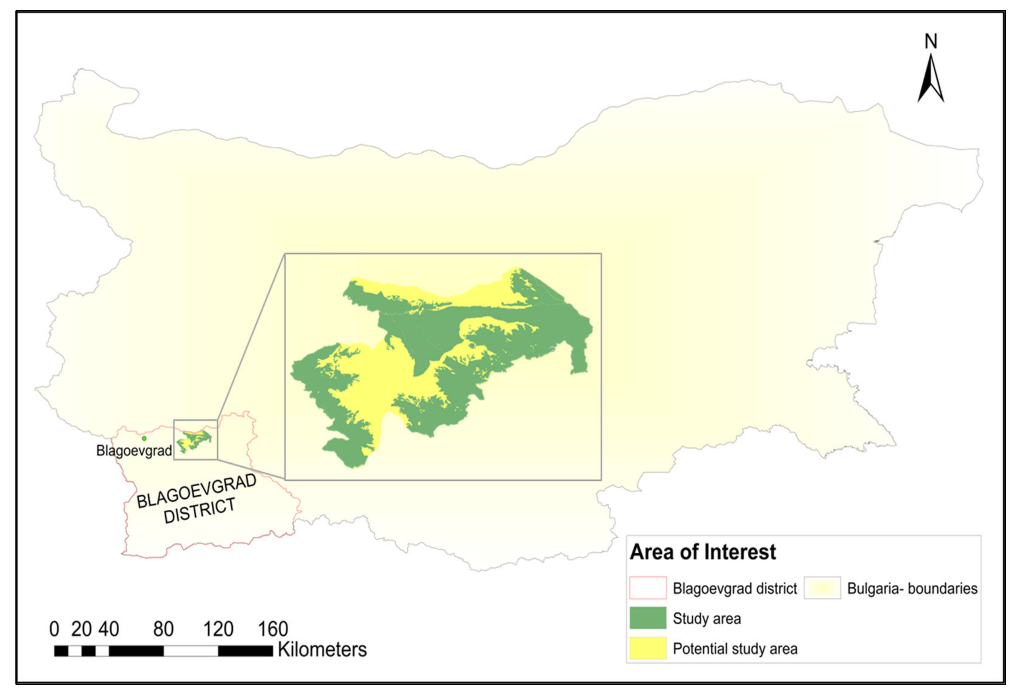
2.1. Study Area

The selected study area is located in the southwestern part of Rila Mountain, Bulgaria (Figure 1). It has a total area of 14,334 ha and includes parts of the communal lands of several populated settlements in Blagoevgrad District, as well as the Parangalitsa Reserve which has been assigned as a reserve since 1933 and was later included in the National Ecological Network Natura 2000 as a protected area for birds and habitats. The highest point of the study area is Dzherman peak (also called Ezernik, 2485 m). Its main ecosystems are woodland and forests, shrubs and grasslands as characterized by [50,51,52,53,54]. Small water bodies including Lake Dzherman and the upper stream of Draglishka river (water body BG4ME800R089 as per the River Basin Management Plan of the West Aegean River Basin Directorate, Blagoevgrad) belong to “rivers and lakes” ecosystem type [53]. The steep rocky surfaces near the top contain sparsely vegetated areas [54]. Thus, five of the nine ecosystem types found in Bulgaria are present in the study area. Due to its inaccessibility, harsh climate, the lack of long series of ground data and the limited number of usable remote sensing images, the study area is representative in terms of data sparsity in the context of being rich in biotic and abiotic diversity—traits it shares with many of Bulgaria’s remote wild areas.
Land use is mainly limited to pastoral habitat. Protection measures under the Common Agricultural Policy include subsidy schemes for managed extensive grazing in protected areas within the Natura 2000 network (we verified this using the Copernicus Ploughing layers for 2015 and 2018). While no logging permits are issued in the study area itself, the surrounding forests are logged actively, in some cases beyond the permitted scope—as visualized in the forest website maintained by the Executive Forestry Agency and WWF Bulgaria, which also contains crowdsourced information on irregularities (https://gis.wwf.bg/mobilz/#/23.38057/42.01433/12 (accessed on 17 March 2022).
This study area, although too small for regional or other large-scale assessments, is commensurate with the characteristic scale [55] of the objects of our observation—high mountain ecosystems and ecotones, and their growth patterns and dynamics. Having in mind the availability of ground data on the location of ecosystems, we were able to use the fact-based basic entity approach ([56]) instead of resorting to statistical methods that may increase uncertainty. The study area satisfies three key criteria:
(i)
its scale corresponds to the study objects;
(ii)
it contains the widest possible variety of HME ecosystems and representative forest-grassland and forest-shrub ecotones; and
(iii)
it only covers protected areas so that the impact of other factors, in particular abandoning the grazing or transition from intensive to extensive grazing, would not overlap on the effects caused by climate change and distort the observations.
The selected study area is furthermore a good example of a place with biased and sparse available data. Large scale field verification is limited due to the inaccessibility of the alpine landscape; moreover, field verification through digitalization or combining datasets is difficult to perform and often impossible for older data. Testing our first hypothesis in such an environment is important since in such places it typically is much more difficult to ensure the reliability and reach desired lower uncertainty levels when including them in national or European scale wall-to-wall maps and models.
In addition, the study area illustrates the great variety of scales in available data sources. ERA Interim pixel size is 12 km and the size of our study area is covered by approximately 2 pixels of that model while it also contains over 22,000,000 pixels of very high resolution satellite products. The lack of meteorological data time series makes climate models the only source of information on temperature and precipitation which we cannot derive from other remote sensing data. At the same time, the large pixel size of ERA Interim causes this dataset to be very imprecise at the smaller scale of the actual ecological processes, which in turn increases the uncertainty of any statistical processing (as discussed by Jelinski and Wu [56] in their exploration of the scale problem’s dependence on grain size in the data).

2.2. The Whole System Framework—A Versatile Tool for Data Fusion and Co-Analysis

The Whole System approach regards the ecosystem as a complex of five subsystems—structural (biodiversity, abiotic heterogeneity) and functional (balance of energy, matter and water). As such, it is integrative to the extent of unifying the research subjects of ecosystem functioning (as part of the biodiversity subsystem) and climate change (as part of the abiotic heterogeneity subsystem). Being dynamic, the Whole System framework is furthermore conductive to working with time series by observing the manifestations of the matter balance and water balance subsystems through vegetation indices and the energy balance—indirectly through the changes in temperature and the related evapotranspiration intensity. Therefore, it is possible to use both climate models and remote sensing methods for observing the system level structural and functional parameters within this framework, as presented in Table S1 of the Supplementary Materials.
Our first hypothesis is based on the understanding that, by its design, the Methodological Framework for assessment and mapping of ecosystem condition and ecosystem services in Bulgaria further facilitates wall-to-wall landscape, regional and national data integration on a number of levels in a manner supportive of data fusion and, ultimately, data integration and co-analysis. The layers of compatibility built into the framework are:
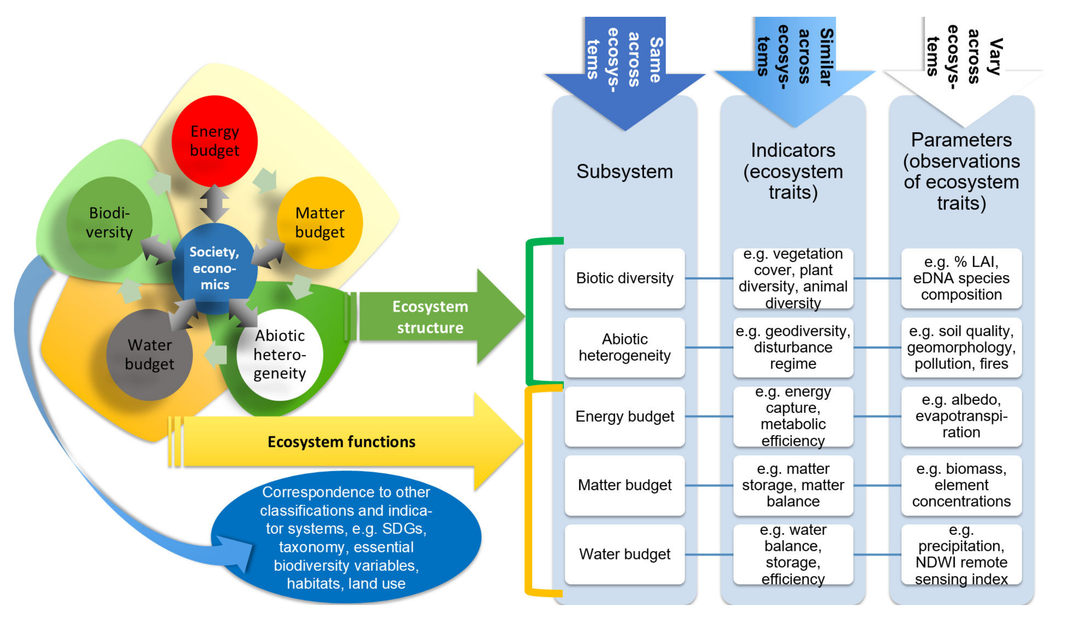
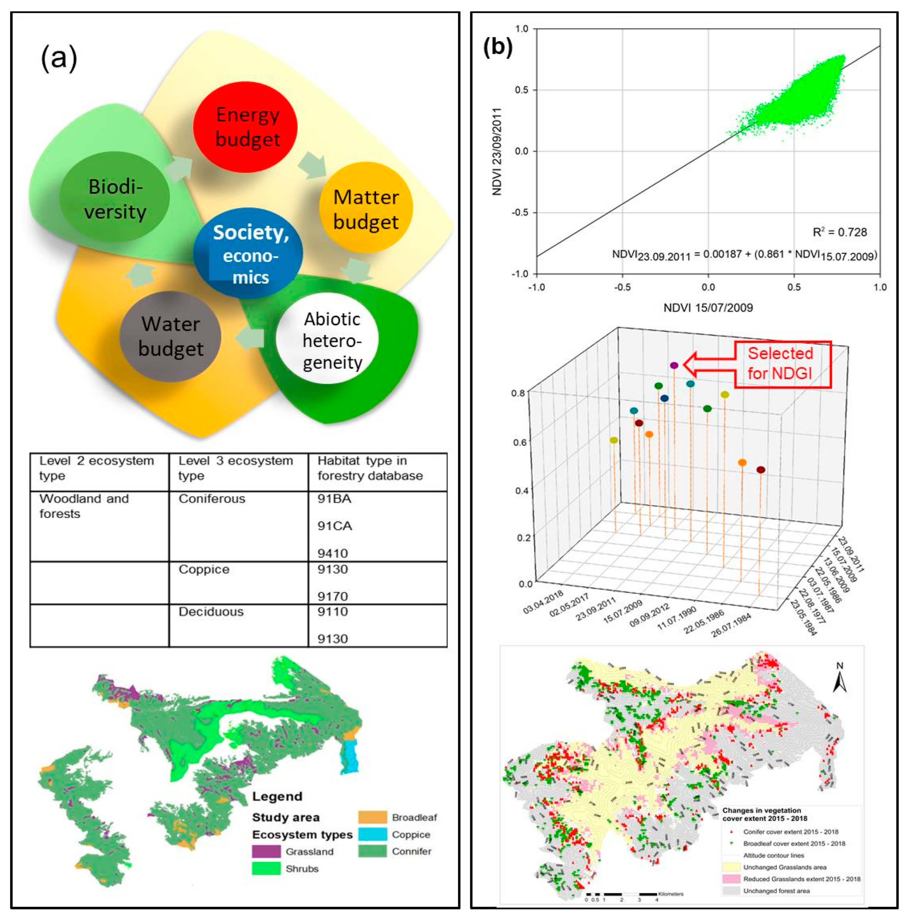
  • Semantic compatibility: This applies the same indicator system to all ecosystems, as detailed in Figure 2. In this manner, indicators vary little across ecosystems, creating semantic links, whereas the huge diversity of observable ecosystem manifestations is mostly contained at the parameter level but clearly linked to the indicators and, through them, to the ecosystem structure or functioning.
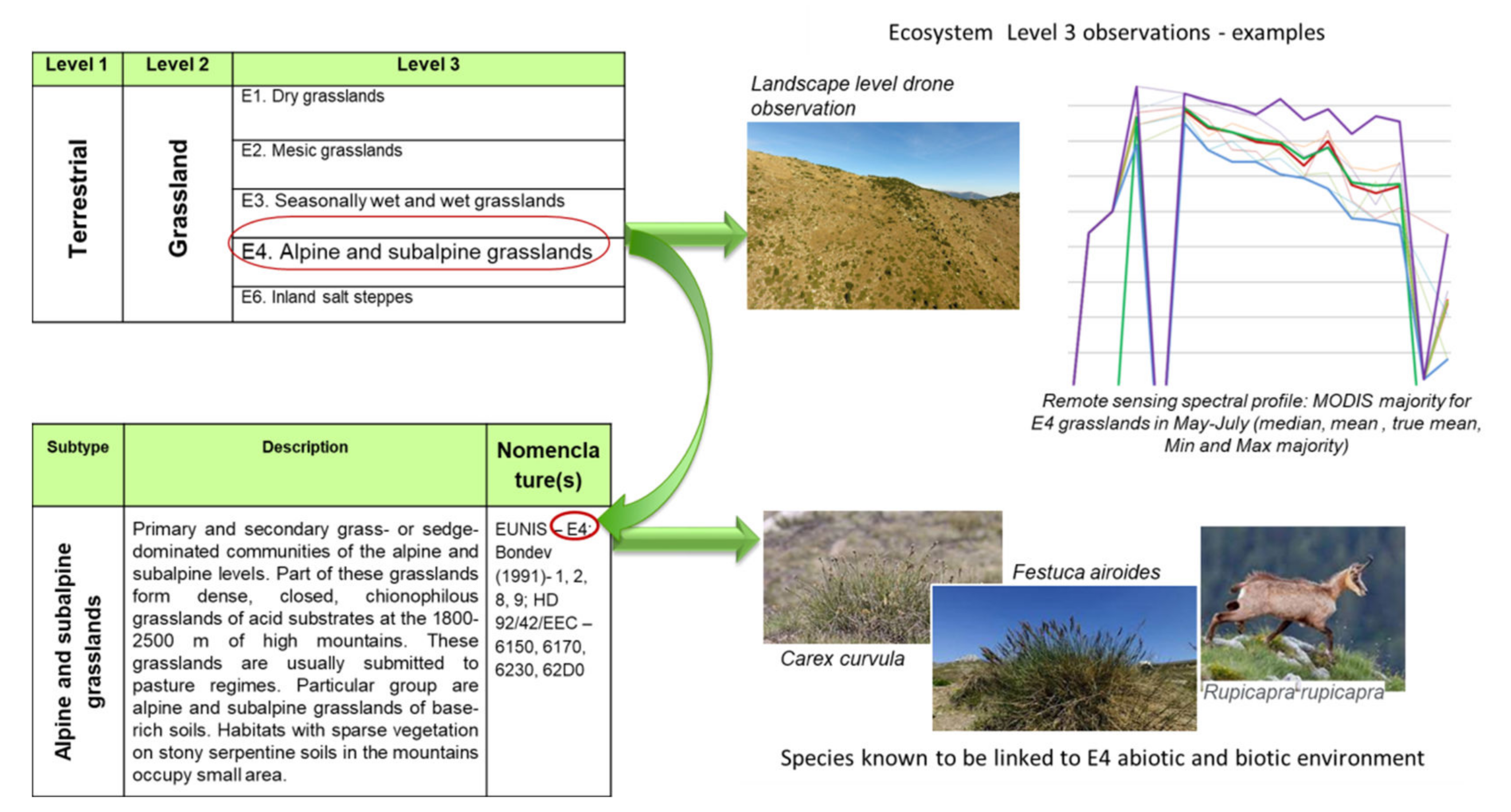
  • Ontological compatibility (for the purpose of this article, we understand ontology not in the philosophical sense but as commonly defined in information technology and semantic web applications as a means for users to create their own set of definitions—in our case, definitions of ecosystem types/subtypes, habitats, etc. Pan (2006) [58] and Serafini and Bogrida (2005) [59] derive mathematical formalism of ontological compatibility and reasoning in the context of decentralized systems such as a multi-ecosystem assessment): Creating links (crosswalks) is another systematic feature of the Methodological Framework. Each Level 2 ecosystem type contains more differentiated Level 3 subtypes (Figure 3). This creates an unambiguous basis for cross-referencing of indicators and parameters collected under reference frameworks as different as ecosystem or habitat classification, plant or animal taxonomies or genetic sequences specific to each subtype. Thus, if lacking ground truth observations, field data collected in another context (e.g., forest inventory including habitat data) about a subset of parameters can be sufficient to find the ecosystem subtype (Level 3), as we demonstrate in this study. Cross-referencing the classification of Level 3 to finer grained ecological concepts such as habitats, while not replacing a detailed assessment, may allow to narrow down the expected habitat types, species composition and other ecosystem traits even with sparse ground data. Moreover, the Methodological Framework includes an in situ verification guide [60] that provides a mechanism for resolving inconsistencies between observations in a landscape, thus addressing the concerns raised by Pan [58].
We note that obtaining ontological compatibility across knowledge domains comes at the cost of losing precision and growing uncertainty [61]. Therefore, automated fusion and processing of datasets matched on the ontological level will be subject to using appropriate mathematical apparatus and methods such as fuzzy logic [62] and fuzzy graphs [63] in the inference of semantic and ontological links and processing of big data.
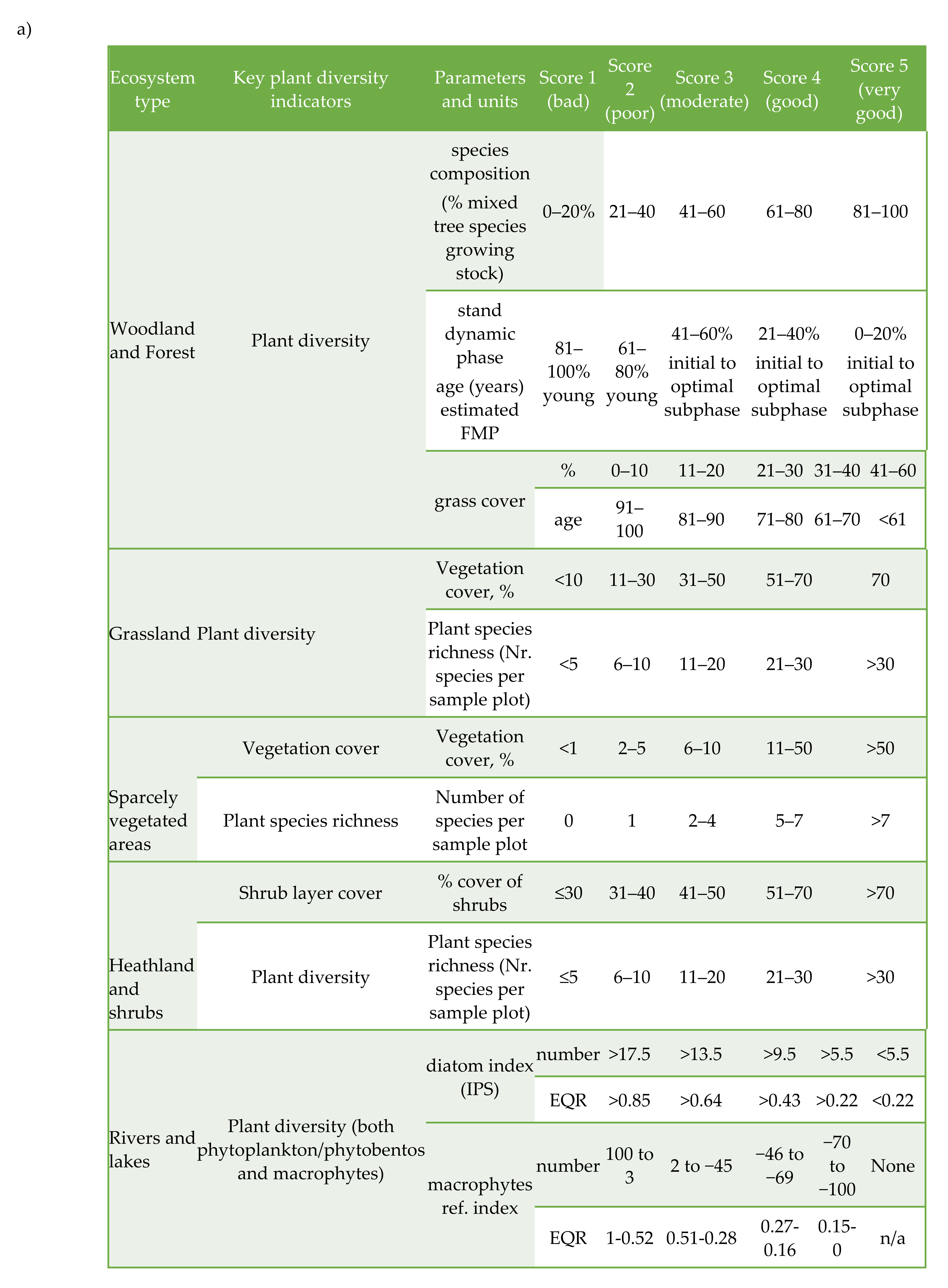
  • Methodological compatibility: One key step of the Methodological Framework is to assign non-dimensional numeric values between 1 and 5 to the ecological parameters and 0 to 5 for ecosystem services (0 being assigned when a service is not provided by this ecosystem). These scores are based on initial expert assessment and later field verification (Table 1). This step ensures the possibility to assess semi-quantitatively different parameters measured using different methods and expressed in diverse measurement units, against the reference values established for different ecosystem condition. Furthermore, the Framework foresees aggregating these semi-qualitative reference values to form single indices for assessing the ecosystem integrity, overall condition and service provision capacity (IP index). Akin to the carbon equivalent in climate change, the IP index both enables a numeric expression of the ecosystem condition/service provisioning capacity, and allows for an overall cross-ecosystem comparison at the indicator or ecosystem level, which facilitates the compilation of wall-to-wall assessments and analyses by IP index or indicator across all ecosystems present on the landscape level.
As with the ontological compatibility, the selected approach to methodological compatibility also introduces a degree of uncertainty and therefore any future automated workflow for data processing may also require the use of fuzzy methods when analyzing and modelling data across ecosystems.
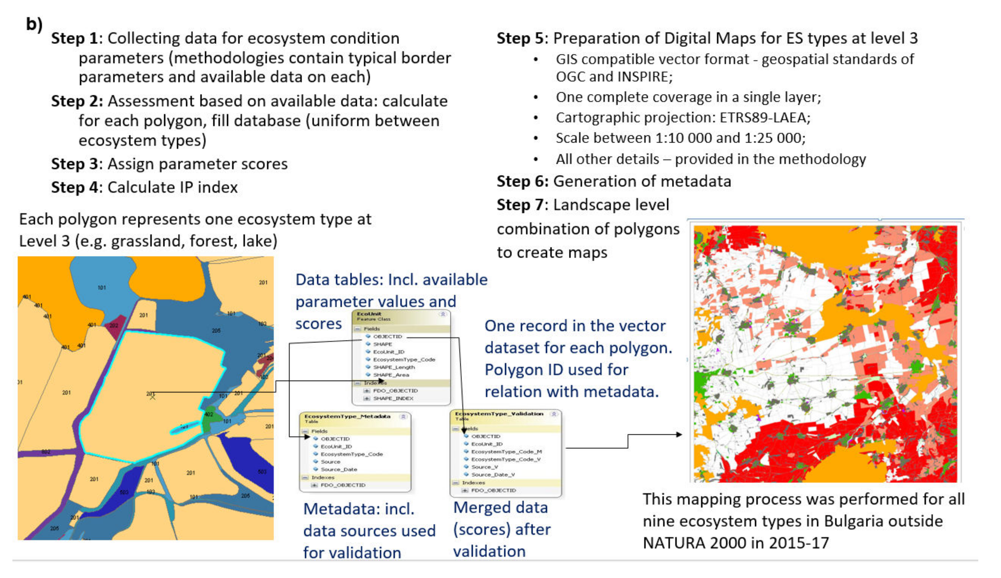
  • Information compatibility: Data reuse is possible by utilizing parameter observations from existing sources, e.g., for forest ecosystems—data from forest inventories; for water ecosystems—monitoring data collected while implementing the Water Framework Directive or Marine Strategy Framework Directive (Figure 4a). In addition, the Methodological Framework prescribes the same database structure and processing workflow in the specific methodologies for assessing each ecosystem type (Figure 4b), hence allowing for a meaningful data fusion [64] from the semantical down to the instrumental level.
  • Extensibility: Incremental improvement within the same framework is key for accommodating changes in research objectives and methods of observation. This is especially important in a time of rapidly emerging new or improved technologies, and is a key test of our first hypothesis.
    To enable data cross-checking, a necessary first step is to match the available datasets to ecosystem parameters and, from there, to condition indicators in the Methodological Framework. In this process, we also assess the existing indicators on their fitness for purpose. The extent and condition indicators for the ecosystems grassland, forest and heathland and shrubs (based on vegetation cover and species composition) are static and therefore by themselves insufficiently informative for assessing the ecosystem extent dynamics over time. This dynamic must, however, be captured in order to cross-analyze it with time series on the climate change parameters and other possible processes influencing the ecosystems such as land management practices or protected-area management plans. This makes the formulation of new indicators necessary. Since establishing these indicators at the national scale is a process beyond the scope of this study, the testing of the extensibility as part of our first hypothesis is limited to formulating candidate indicators based on observations in a single study area.
The sparsity of existing field data is an additional challenge that renders difficult to impossible the application of many of the existing approaches to fusing heterogeneous data to a complete and consistent dataset, as proposed by [58]:
  • Yager [65] implies that there is a single, well-defined variable that can be inferred from different data sources, which is not the case in established literature either with ecosystem integrity or with climate change. While such a variable is defined in the Methodological Framework through the use of IP index, it has not yet been used to characterize NATURA 2000 protected areas (including our study area).
  • The too large scale of data derived from climate models (effectively the entire study area is covered by a small number of pixels) makes them too coarse for automated processing until reliable downscaling is developed—a problem faced even in data rich areas like the cities that need more detailed projections to tackle urban heat islands (the difficulties of downscaling climate models are apparent from the dataset Climate Variables for Cities in Europe from 2008 to 2017—a project that required standalone modelling, has higher local uncertainty and is apparently no longer maintained. The dataset is available online at https://cds.climate.copernicus.eu/cdsapp#!/dataset/sis-urban-climate-cities?tab=overview (accessed on 17 March 2022)).
  • Automated data fusion through machine learning or AI typically uses high-resolution images or consistent single-ecosystem data series [66,67], or performs experiments with ground truth knowledge in curated datasets [68,69]. The latter also perpetuate bias in algorithmic data fusion by being highly anthropocentric (such as [70], and the datasets quoted therein, US Merced (http://weegee.vision.ucmerced.edu/datasets/landuse.html (accessed on 17 March 2022))), focused on ground truth labeling a single ecosystem [71,72] or generally labeling a single variable for a given task ([73], the Brazilian coffee dataset (www.patreo.dcc.ufmg.br/downloads/brazilian-coffee-dataset/ (accessed on 17 March 2022), etc.). In contrast, our remote sensing data is sparse, of different resolution over time, heavily biased and does not form a regular data series that covers the annual vegetation growth cycles. Its ancillary ground data is also sparse and biased. Furthermore, landscape level classification including more than one ecosystem type is more difficult algorithmically due to additional bias caused by the different scale or area of landscape features representing different ecosystems and their representation in a limited number of satellite bands. For example, rivers and small landscape forms, like small woody features occupying in some cases less than one pixel, need specific extraction different from the processing of remote sensing data for vegetation massives like forest and grassland; these are in turn less homogeneous than cropland monocultures. Finally yet importantly, its land cover (and the seasonal land cover dynamics) is quite different from the existing labeled datasets, so transfer learning would be difficult to impossible.
Due to these limitations, in this study we resort to joint semi-quantitative analysis of existing data sources as detailed in the following sections. Automating the method through a consequent implementation of fuzzy graph analysis is the subject of ongoing research, and therefore outside the scope of this study.
The Methodological Framework focuses on fieldwork or other existing terrestrial data while it mainly uses remote sensing information such as ortho-photo for visual inspection and study object identification at the preparation stage prior to fieldwork. This approach, however, causes a number of qualified scientists to become a bottleneck for large-scale data collection, leading to data deficits, particularly in inaccessible or difficult study areas like ours. In the currently accepted parameter system and its respective protocols, there are no parameters based on vegetation indices or modeling (including climate change reanalysis). Thus, the existing indicator and parameter system of the Methodological Framework is well suited for mapping and assessment but not for continuous remote monitoring. This poses another significant challenge in data sparse and/or inaccessible areas. Therefore, our current study contributes to extending the Methodological Framework by proposing a means to complement it additively with back-up methods for continuous remote monitoring in sparse data environments (as detailed in sections Results and Discussion).
The Methodological Framework was developed in 2015–2017 before some significant developments in the mapping and assessment of ecosystem services at the global and EU level (such as the 2020 revision of the System of Environmental Economic Accounting (https://seea.un.org/content/seea-experimental-ecosystem-accounting-revision (accessed on 17 March 2022)) and the development of a systematic supply and demand spatial analysis for ecosystem services led by the EU’s Joint Research Centre [74,75]). It therefore lacks the conceptual basis for ecosystem extent and condition accounts and the supply side of ecosystem services is insufficiently linked with the demand side. Against this background, we emphasize the extent and condition assessment as two important elements of extensibility when testing the first hypothesis in this study.

2.3. Data and Its Processing

Based on the Whole System approach outlined above, we test our first hypothesis by attempting to use all available data to the extent possible. Therefore, we collected heterogeneous data outlined below, and did not exclude any data available to us based on metadata only (e.g., due to insufficient spatial or temporal resolution). This scope used data wider than in studies that focus on a smaller number of datasets. Our approach is to seek ways to ensure, for each available dataset, as a minimum semantic, but ideally also ontological, methodological and/or information compatibility. The data selection process also ensures that we aim at achieving at least partial data availability for the ecosystems’ biodiversity, abiotic structure and functions across all five subsystems of the Whole System. We deem data to be similar in the temporal scale if the observed ecosystems’ phenomena remain stable between two data points. For example when exploring phenology, similar data are the data collected within the same vegetation stage, whereas, when studying succession, the similar data may include data points collected within 2 or even 5 years. We derive such timeframes for the different ecosystem types based on the Monitoring Guide [76] of the Methodological Framework. For the purpose of our study, data from Copernicus products for base year 2018 and data on the most dynamic meadow ecosystems from the forestry database (2016) are less than 3 years apart and therefore we consider the two datasets essentially similar across all ecosystems. If considering only slowly changing ecosystems like forests, this interval may be even larger. Grounds for excluding a data item or dataset may be its redundancy to more detailed or reliable data, or its proven high uncertainty when cross analyzing with other data. Still, the exclusion of data is rather the exception and not the rule in our data fusion method. Such an all-inclusive approach to data collection and processing is important for uncovering synergies between datasets; there is also the important emergent effect of ecologically meaningful reanalysis of multiple datasets to improve the overall analytical quality or spatial/temporal scale.

2.3.1. Field Data

As a main source of information, we used official partial forestry inventory data in GIS format (Executive Forestry Agency, 2016) to distinguish the main ecosystems on the territory of the study area. This data includes information on non-forest formations such as meadows, and was therefore suitable to delineate spatially the ecosystem types. Since mapping and assessment of ecosystems within Natura 2000 protected areas has not been performed yet in Bulgaria, for the ecosystems other than forest we used a variety of other available data sources:
  • data from the official agricultural subsidy layers for High Natural Value pasture grasslands eligible for funding and actually funded (since 2015) (State Agriculture Fund, access rules at https://www.dfz.bg/bg/selskostopanski-pazarni-mehanizmi/school_milk/doc-up-uml-3-2/ (accessed on 17 March 2022))
  • data from the surface water monitoring under the Water Framework Directive as contained in the River Basin Management Plan 2013–2015 (A central database is maintained by the Executive Environment Agency, more at http://eea.government.bg/bg/nsmos/water (accessed on 17 March 2022) (in Bulgarian only))
  • field photography data obtained by the lead author using a drone in the period 2016–2017
  • publications (Bondev, 1991) [77] as digitized in 2013; other scientific publications on ecosystem condition for the study area
  • soil map (Executive Environment Agency) (the metadata for this dataset is available at http://eea.government.bg/bg/nsmos/spravki/Spravka_2020/soil (accessed on 17 March 2022) (in Bulgarian only)
  • real-time forest information system maintained by the Executive Forestry Agency and WWF-Bulgaria and containing data on old forests, land use mode, logging permits and crowdsourced information on irregularities reported by volunteers (view at https://gis.wwf.bg/mobilz/, accessed on 17 March 2022).
We found a strong bias both in the research and administrative efforts made to inventory the different ecosystem types. Forest ecosystems are subject to routine data collection, and their growth, disturbances and pests are much better studied and mapped with a relatively high level of detail on species composition (dominant species and up to 7 other species are being entered). In contrast, much sparser data was available in the forestry database on ecosystems other than forest, except for the heathland and shrub ecosystems also classified under the EU Habitats Directive as habitat 4070—bushes with Pinus mugo and Rhododendron hirsutum. In contrast, the only description of grasslands as “meadow” is very broad. Data on the availability of alpine and subalpine grasslands outside the forest management area are insufficiently georeferenced (either due to missing coordinates or due to coarse scale mapping). In the sense of data integration, this limited the scope of much of the present analysis—determining Level 3 ecosystem subtype had to be constrained to the spatial–temporal trends in the parts of the study area inventoried in the forest management databases (colored in green in Figure 1). At this time, the only practical way to classify ecosystems in the remaining part of the potential study area (outlined in yellow in Figure 1) is to resort to Level 2 classification as the use of remote sensing and climate data requires additional ground truth validation by a larger team.
The study area is subject to vivid scientific interest with over 100 publications. However, there is a strong disparity of study objects on the ecosystem level, with prevailing forestry studies and scarcely any publications on the grassland, sparsely vegetated or river/lake ecosystems. Forestry publications taken into consideration include forest condition assessments, climate studies fieldwork, water balance and pollution studies; we discarded species level papers focusing on single species of flora, fauna or fungi, which form the bulk of the publications. Particularly relevant to our study are publications on the condition of forest ecosystems, including publications on large-scale disturbances causing changes in condition or functioning that may influence the vegetation index values [78,79,80,81,82,83,84,85]. These sources show that windthrows seem to be the major cause of disturbance. To further specify the classification of ecosystems across the study area, we restored to the crosswalks defined by Kostov et al. (2017) [50], Velev et al. (2017) [51] and Apostolova et al. (2017) [52].

2.3.2. Remote Sensing Data and Products

In this study, we use three types of remote sensing data: Ortho-photo data (2013) (Data upon request, GIS viewer at http://gis.mrrb.government.bg/ (Bulgarian only) (accessed on 17 March 2022)), satellite derived expert products to determine the current ecosystem extent and a long time series of remote sensing scenes as means to derive vegetation indices to assess ecosystem condition. This section lists and describes the data while details of data processing to overcome the shortcomings in each product type are provided in Supplementary Materials, Section S5.
Expert products are better suited for static features such as the positioning and characteristics of specific vegetation types. They are released in a sparse data series (for Copernicus—typically every 3 or every 6 years, depending on the product) and their production involves significant processing and quality control that does not need to be repeated by the authors. A shortcoming of expert products is that they do not provide complete (wall-to-wall) coverage but focus on single ecosystem types and therefore their joint use leaves gaps when pixels do not belong to any of the ecosystem types in the respective products.
For ecosystem extent, we chose the Copernicus High Resolution Layers (HRL) expert products for grassland (grassland extent layers) and forest (tree cover density and dominant leaf type), the two products that, taken together, provide the most coverage in our study area’s landscape, while also distinguishing between dominant forest type and detailing the tree density. We chose reference years 2015 and 2018 since these are the only two reference years available for both the grassland and forest HRLs.
In contrast, remote sensing scenes are processed to a much lesser extent (e.g., orthorectification, cloud removal, etc.) but are available on average once in two to three weeks, which makes them suitable for forming longer, seasonal data series to perform functional observations or confirm vegetation location to explore spatial extent.
On ecosystem condition, we performed a selection of vegetation indices (VIs). Essentially, VIs are based on the reflectance properties of the vegetation and are designed to measure vegetation quantity and vitality in different aspects—canopy area and structure, concentration of chlorophyll [86]. For the long-term condition and functional assessment of the selected HME in Bulgaria’s Rila Mountain, we applied an empirical method based on two well documented vegetation indices (the Normalized Difference Vegetation Index (NDVI) and Normalized Difference Water Index (NDWI) [87]) as well as the newly developed Normalized Difference Greenness Index (NDGI) [88]. Research on the relationships between NDVI and climatic variables already enables predictions and trend definitions [89], albeit at much larger scale.
We selected for use of multispectral satellite data from MultiSpectral Instrument (MSI) sensors of Landsat from the United States Geological Survey (USGS) database covering 42 years (1977–2019) and Sentinel 2 data with high spatial, spectral and radiometric resolution [90].

2.3.3. Climate Data

In our study, we use climate data for the parameters ‘t2m’ (temperature 2 m above ground level), ‘tp’ (total precipitations), ‘evpt’ (evaporation) and ‘v10’ (10 m V wind component) extracted from the public daily subset of the ECMWF Re-Analysis (ERA Interim) dataset of the European Centre for Medium-Range Weather Forecasts (ECMWF) database.
The multidimensional files in NC format contain information for each parameter within the vegetation periods (May–September) for most of the studied period—40 years from 1979 (the starting year of ERA Interim reanalysis time series), to the time series’ end in August 2019. We prepared these NC files for further use by ArcMap 10.3 processing. We produced raster files of each parameter for every month within the vegetation period for the 40 years of climate simulations and converted them into shapefiles to facilitate data extraction. We extracted the attribute data and transferred it to SigmaPlot 11.0 where we performed the regression and line plot analyses.
The retrieval and processing of climate data also has some limitations. ECMWF discontinued ERA Interim—the dataset containing relevant variables for our study in August 2019. It provides the follow-up reanalysis dataset ERA 5 [91] in stages and currently ERA 5 is only available starting 1981. In addition, it had some errata and is still being verified across the globe [91,92,93] with no verification yet for Europe on all climate variables needed for replicating our study using ERA 5 data.

2.3.4. Data Processing Workflow

Processing of Single Datasets

The remote sensing data preprocessing steps include:
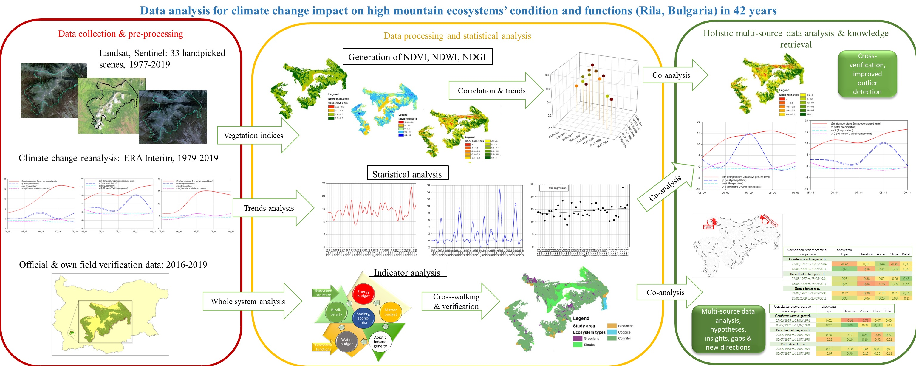
  • Review and selection of scenes from both sensors. While satellite missions regularly fly over our study area, it often is cloudy or misty, and in some years there is snow in parts of it well into May. Therefore, we had to handpick suitable scenes (listed in Table S4 in Supplementary Materials). Unfortunately, these scenes do not adequately cover all vegetation seasons with satellite imagery. Even in the handpicked scenes that we analyze in this study, there are still some clouded areas (visible in the false color renderings in Figures S7e, S9d, S10a,d, S12a,h, S13d and S16d,g,j of the Supplementary Materials and Figure 5). Based on cloud coverage masks over the study area and additional visual review, we selected a set of 33 satellite scenes with minimal to no cloud coverage, taken within a time frame of 42 years;
  • Creating composite images containing spectral bands of the images. In this step we used ERDAS 14.0 software.
  • Creating a raster file of each scene containing the Area of Interest (AOI), i.e., study area boundary.
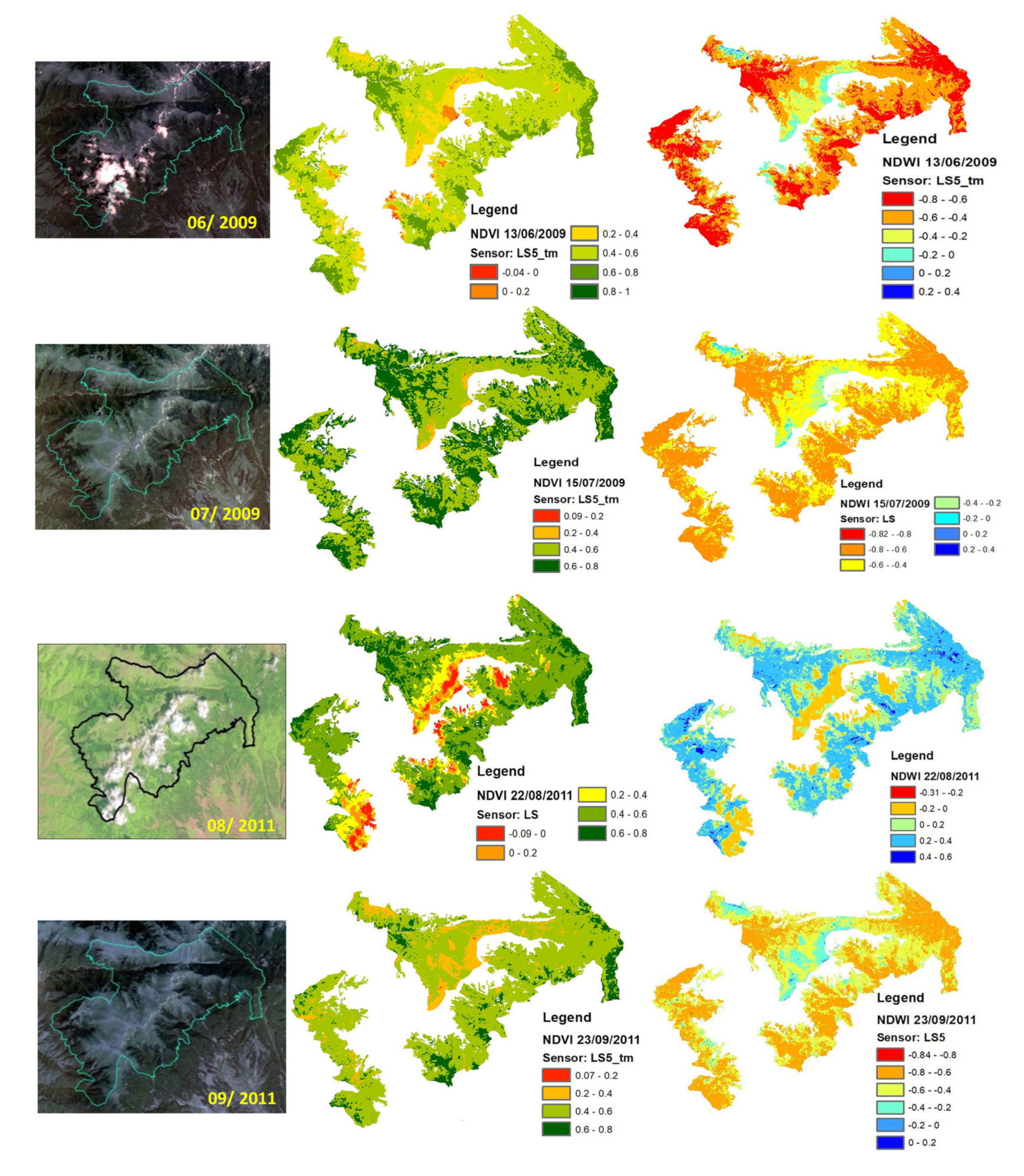
  • Calculation of VI from the selected scenes. We calculated Normalized Difference Vegetation Index (NDVI) for all 33 scenes and produced raster files. Older Landsat sensors with fewer bands do not allow calculating NDWI and therefore in 12 of the Landsat MSI satellite scenes we could not obtain the values of this index.
Table S4 of the Supplementary Materials contains a summary of the data provenance of the satellite scenes used in the study.
NDVI is the most widespread index for vegetation condition assessment indicating its energy absorption and reflectance capabilities, photosynthetic capacity and biomass concentration [94,95,96,97]. According to Pettorelli et al., 2005 [89], “it could be used to predict the ecological effects of environmental change on ecosystems functioning”.
To clarify the relationship between climate parameters and NDVI values and define their influence on NDVI values within the studied period (1977–2019), we analyze the VIs of single scenes within a vegetation season together with the available climate data. We aim at inferring trends of condition changes for the HME in the study period.
We visualize the distribution of NDVI through 3D graphics including the index values for the forest within the HME as a whole. Because of the large data volume, the elaboration of a single 3D graph for this period is challenging, both computationally and visually. Therefore, we constructed six 3D graphs (Figure S6 of the Supplementary Materials) containing NDVI data from dates in the beginning (Figure S6a,b), in the middle (Figure S6c,d) and in the end of the period (Figure S6e,f) to present the distribution of NDVI values. We based the data grouping by dates on calculation of correlation coefficients between NDVI values in the satellite scenes.
After the calculation of the VIs, we prepared 33 thematic maps (TM) of NDVI, 21 TM of NDWI and 5 TM of NDGI using ArcMap 10.3, as well as six 3D graphic models using SigmaPlot 11.0.
Since our satellite time series is composed of images from several satellite missions with different sensor characteristics that influence the respective NDVI values, we cross-verified the results using the sensor-invariant Normalized Differential Greenness Index (NDGI) [88]. NDGI is a dynamic index calculated for pairs of satellite scenes in remote sensing time series and therefore suitable for change detection and verifying the changes in vegetation conditions in situations where NDVI from different sensors may not be fully compatible between scenes. It is very sensitive to even small increments of vegetation development; furthermore, it is designed to detect changes in vegetation cover for a specific time interval, which makes it useful for vegetation processes (photosynthetic capacity), i.e., vegetation functional assessment. Based on the spectral reflectance characteristics of the vegetation, this index is defined through the greenness component obtained via orthogonalization of the satellite images. Using the greenness component causes NDGI to be sensor and time invariant. Furthermore, the error stemming from external factor influences during satellite image capturing is significantly diminished [88]. The index values range from −1 to +1, where the negative values (NDGI < 0) correspond to a decrease of the vegetation process (loss of vegetation) and the positive values (NDGI > 0) indicate an increase of the vegetation process, i.e., photosynthesis takes place (appearance, development of vegetation). When NDGI = 0, biomass production remains unchanged for the studied period.
Due to the limited number of available cloud free scenes, we only generated five NDGI TMs (Figure 8). Four of them have a full set of correspondent climate parameters for the years in which the starting and final scenes of the NDVI comparison were taken. For the period 1984–1977, we lack the climate parameters for 1977 to compare with NDGI. We assessed the suitability of scene pairs for calculating NDGI based on correlation analysis.
For Copernicus HRL products, we performed GIS-based analysis and identified areas of interest based on the different attributive information in pixels with the same location in 2015 and 2018 to identify changes over time. We used this data to localize changes in extent for grassland and forest ecosystems, as well as changes in species composition in forests.
For the retrieved climate data, we extracted the single variables of interest for each month and performed regression analysis on them. Figure 5 presents a sample of the results, for the variables t2m and tp in the months of June and July during the period 1979–2019, while the full range of climate data time series plots and regression analyses for tp is available in the Supplementary Materials (Figures S1–S5).

Cross-Validation of All Available Data

We use the Whole System paradigm to organize data and jointly analyze different high mountain ecosystems in our study area and the different datasets available from their measurements. To this end, we re-compiled a table of combined data sources complementing the parameters in the Methodological Framework (for a list of indicators common across the ecosystems see Table S1 and for their availability in the ecosystems in our study area Table S2 of the Supplementary Materials). We furthermore perform the following analyses:
  • At the semantic level, we explore relationships between potential new parameters derived from remote sensing and climate models, and the indicator they describe. This approach allows for identifying and proposing alternative observation techniques for the same indicator (see Table S3 of the Supplementary Materials). Cross-calibrating such data sources to identify their accuracy, measuring ecosystem parameters can help to establish them as alternatives to field observation data (the standardization of observations for different ecosystem types is part of ongoing work in the European Long-Term Ecosystem Research Network and globally in several initiatives. As such, performing it is currently outside of this paper’s scope). Furthermore, complementing the Methodological Framework with Earth observation and climate modelling allows us to look at a larger scale landscape mosaic and easily locate the most dynamically changing areas of interest such as the forest ecotone or areas with rapid changes in species distribution. In this manner data co-analysis at the semantic level allows for using the synergies between available data from all sources to both observe changes in the whole area of interest and identify focus areas for observation efficiency, both within the same conceptual framework. The semantic linking also allows us to combine data mostly related to ecosystem extent and data typically used to study ecosystem conditions by applying ecological knowledge to infer the links between extent and condition.
  • At the ontology level, we verify/specify the crosswalks between habitat type data in the forestry database and ecosystem types, as applicable to this specific study area. The crosswalks are established as a one-to-many relationship in the respective ecosystem mapping methodologies—parts of the Methodological Framework [50,51,52,53,54]; see Figure 6a. Verification consists of a georeferenced view of available data for habitats and an on-the-spot check of respective ecosystem type/subtype having in mind the overall ecosystem structure. The level of detail of the crosswalk depends on the relations of different labels of available data according to different classifications in the crosswalk. For example, the finer grained habitat labelling of a polygon allows for deducing the coarser ecosystem subtype or type classification for the same polygon while data on the ecosystem type does not automatically translate to ecosystem subtypes or habitats and typically requires further field validation and/or co-analysis with other available data. Heathland and shrub ecosystems are specified in the forestry database to have Pinus mugo as their dominant species and were therefore assumed to be of the “Arctic, alpine and subalpine shrub” ecosystem subtype. To overcome the limitations of existing data on grasslands, we analyzed the forestry database’s information on elevation, slope, exposition and soil types (the latter being also verified using the classification in the Executive Environment Agency’s soil type layer). We then defined the possible ecosystem type as Alpine and subalpine grasslands based on Apostolova et al. (2017) [52] and an unpublished interpretation key produced during the mapping and assessment of grassland ecosystems in 2015–2017 by the same authors.
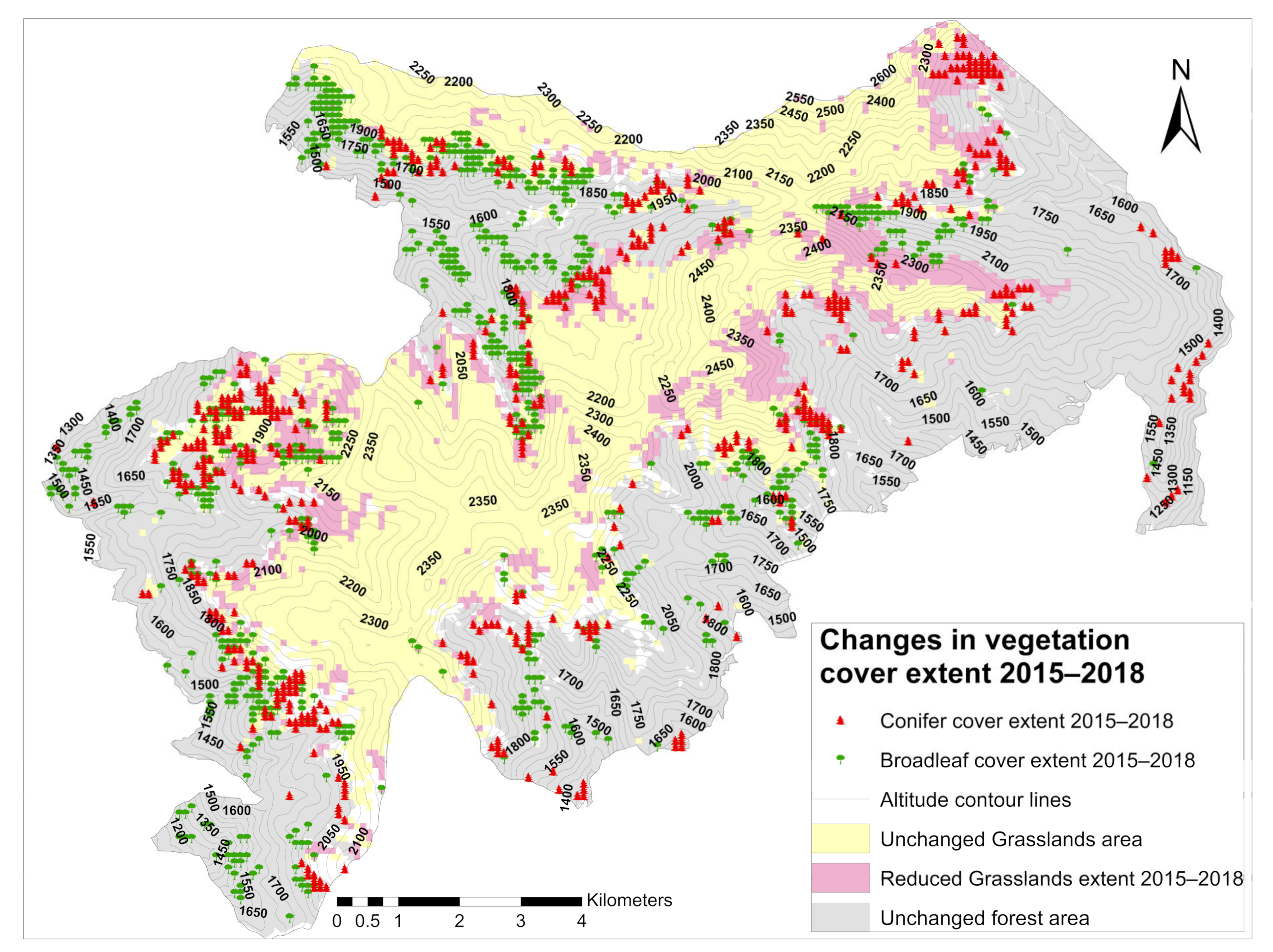
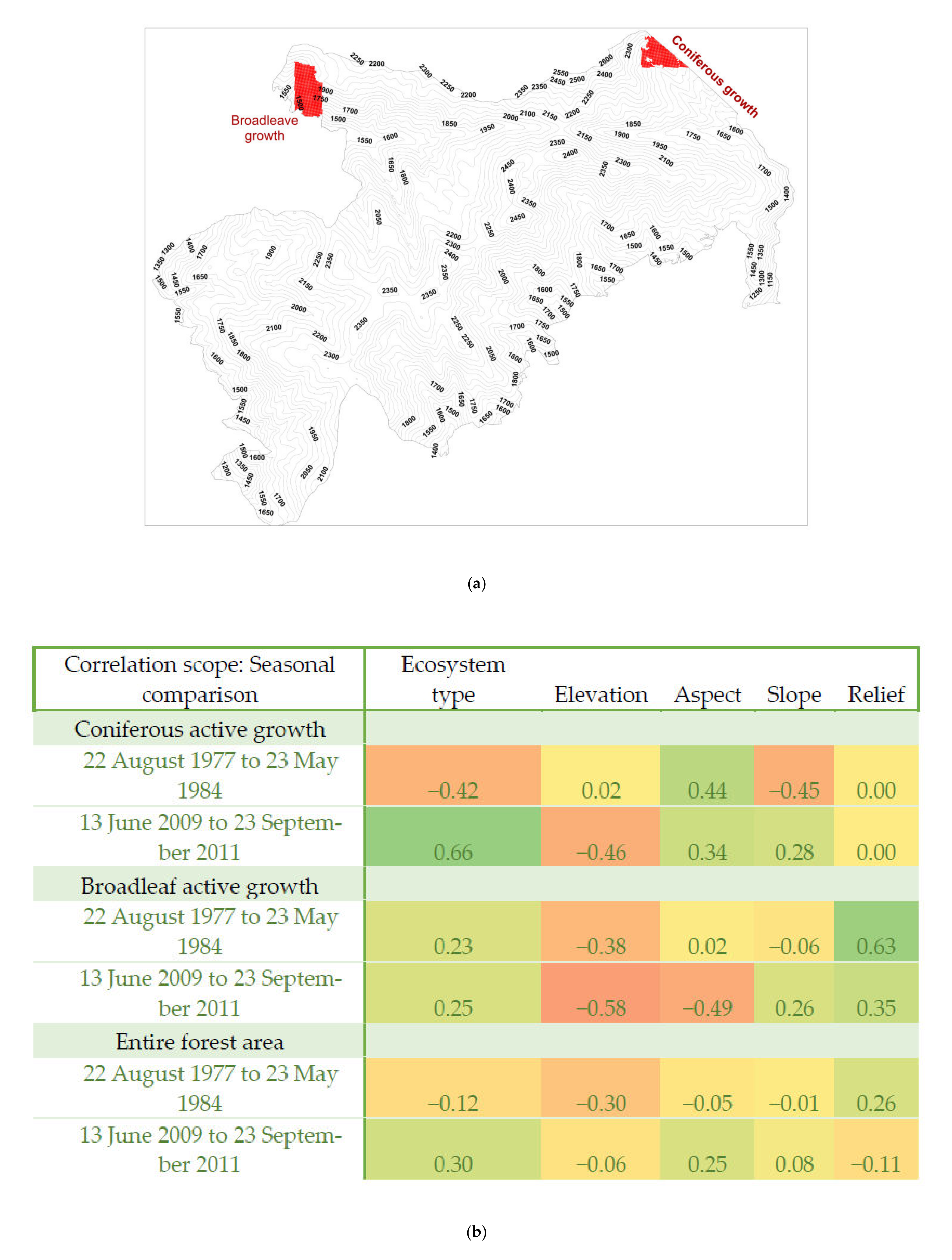
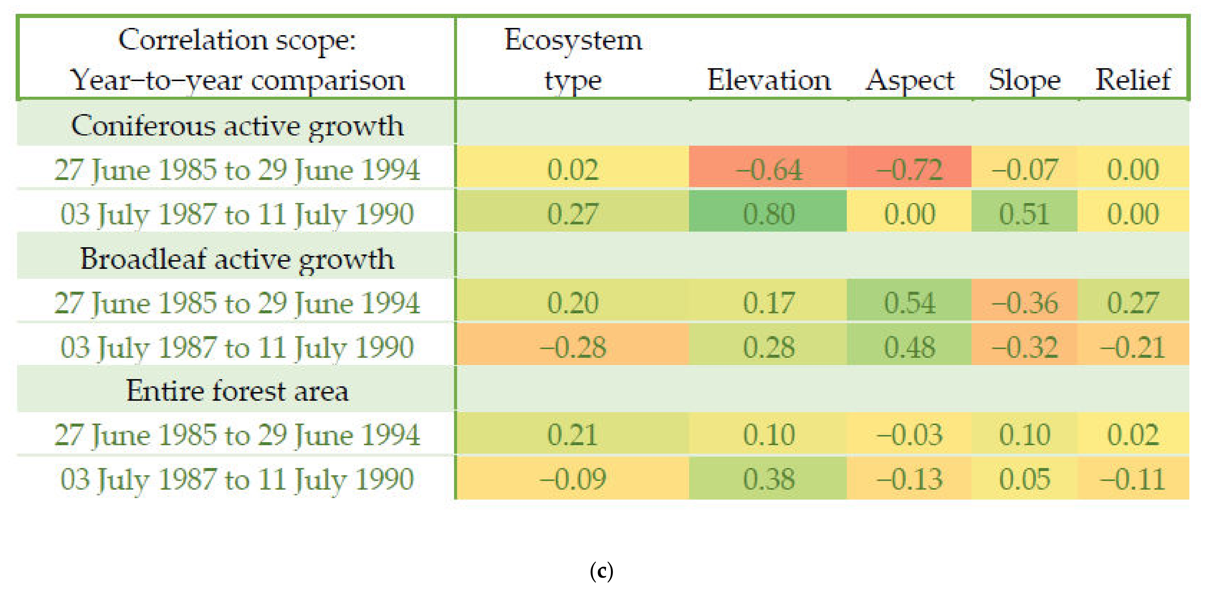
  • At the methodological level, we fuse semantically and ontologically compatible datasets to verify the hypothesis that climate change causes changes in ecosystem spatial distribution within the landscape mosaic and ecosystem condition/functioning over time, including change in species composition. We use the spatial distribution of ecosystem types in this crosswalk derived from ortho-photo and forest database data, together with Copernicus HRL products for grassland distribution and forest tree cover density for 2015 and 2018 to geolocate areas of recent location and dynamically changing composition of ecosystems in the landscape. In the resulting mosaic (Figure 6b, bottom), the data fusion of remote sensing and climate data conforms to the ground truth observations concerning the dominance and location of forest ecosystems. The highest parts of the study area are covered with shrub vegetation and grasslands, which are unevenly distributed, covering sub-alpine and alpine territories. Following the crosswalk validation, we combined data from the different available sources to form time series in the sequence depicted in Figure 6b. We performed a correlation analysis of the NDVI TMs generated for the satellite images to analyze the spatial correlation of NDVI across satellite scenes and find pairs of scenes of analytical interest (Figure 7). This data is complemented with ecosystem location and species composition towards the end of the period, as derived from ground data and Copernicus HRL.
  • Having in mind the need to update the Methodological Framework with developments that occurred after its publication, we furthermore used the co-analysis of climate and spatial distribution data from satellite products to derive reference values for candidate indicators based on remote sensing and thus test the framework’s extensibility.
Using all available data on both extent and condition proved necessary for the reanalysis of data in the earlier part of the study period and therefore complements the missing or insufficiently detailed ground data on the beginning of succession in the forest–grassland ecotone, as well as the upward crawl of deciduous species, causing the change in species composition in forests. To verify the data fusion, we defined that the datasets for spatial extent must contain georeferenced data on ecosystem existence at least at Level 3 (ecosystem type) but preferably at ecosystem subtype or habitat level. Data on ecosystem condition must relate to condition and functional parameters over time, such as biomass production observed via the proxy of vegetation indices. The stages of cross-validation at the methodological level are detailed below:
(1)
We performed a combined analysis of NDVI and where available—also NDWI to verify the observed vegetation growth in each scene. A sample of such results is presented in Figure 7, while the full set of processed images is available in the Supplementary Materials (Figures S7–S16 and S18). This approach is necessary due to the chosen scale of observation—in contrast to expert products that cover all of a given ecosystem type but do not contain its dynamic characteristics, factors like clouds render parts of the few available scenes unusable, which only allows partial processing of these scenes.
(2)
We analyze the derived vegetation indices (NDVI and where available—NDWI) for each year together with climate data for the respective vegetation season to observe the ecosystem functioning and its relations to the climate parameters in the respective year. Since the climate reanalysis does not yield detailed projections, the only way to observe the influence of local parameters determining the microclimate, such as elevation, slope, aspect, is by comparing the geolocated vegetation indices in scenes from different stages of the vegetation period with the data on abiotic factors derived from the forestry database. At this stage, we perform this analysis in a qualitative manner.
(3)
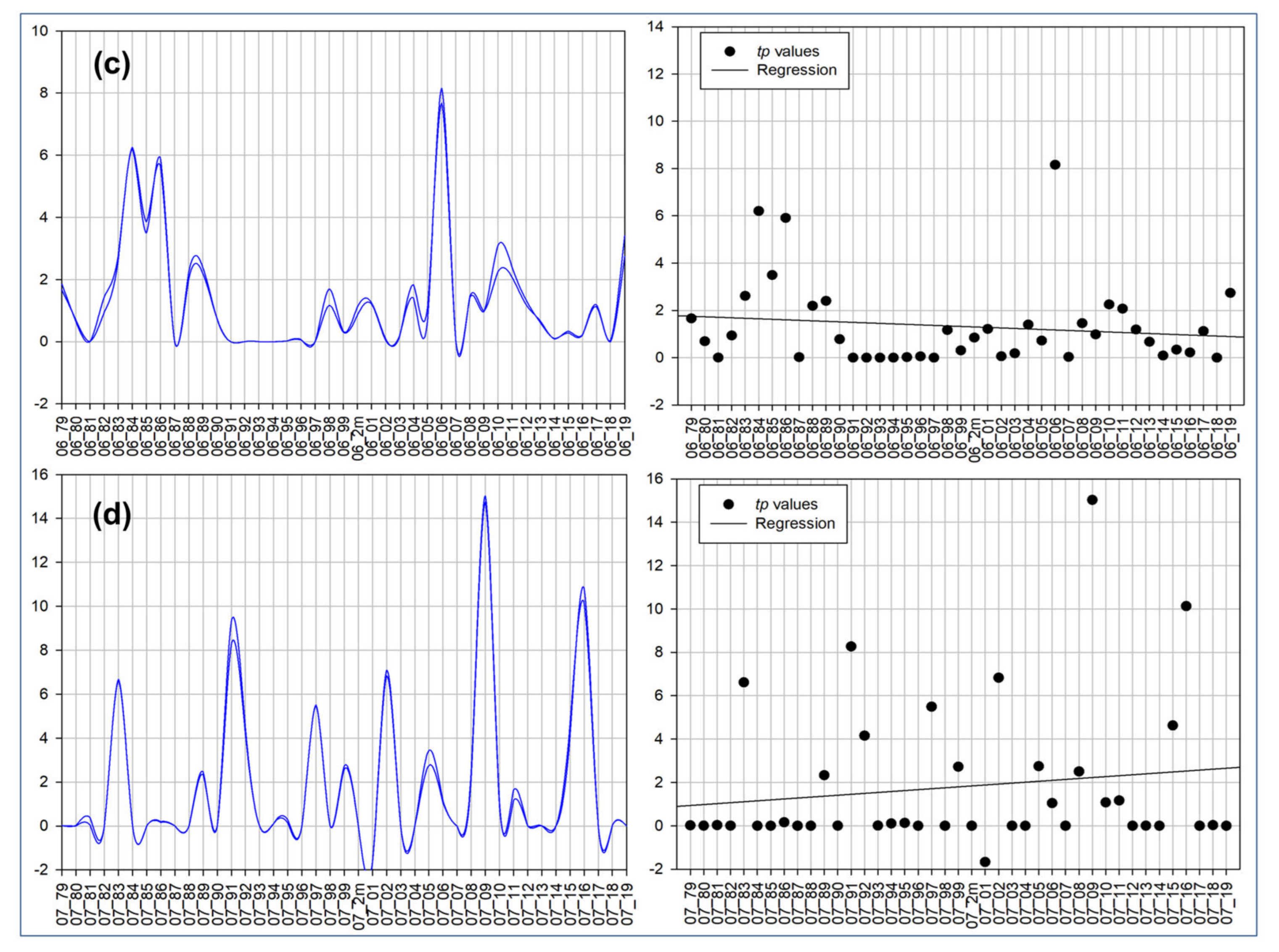
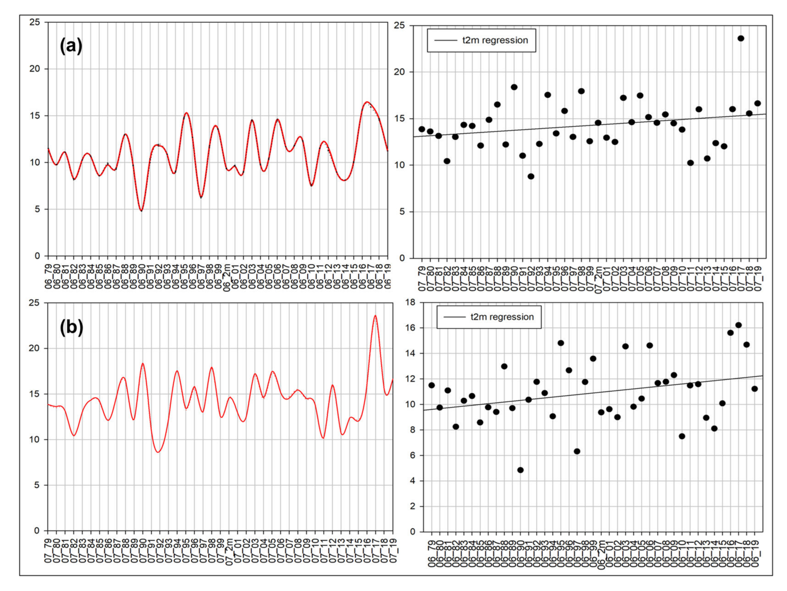
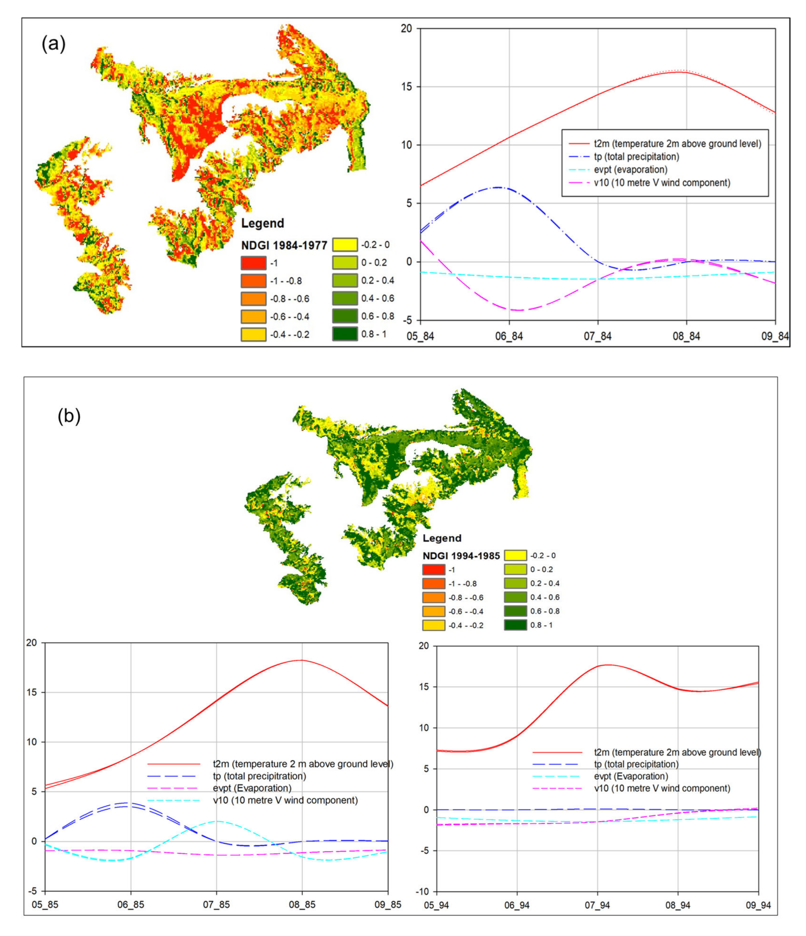
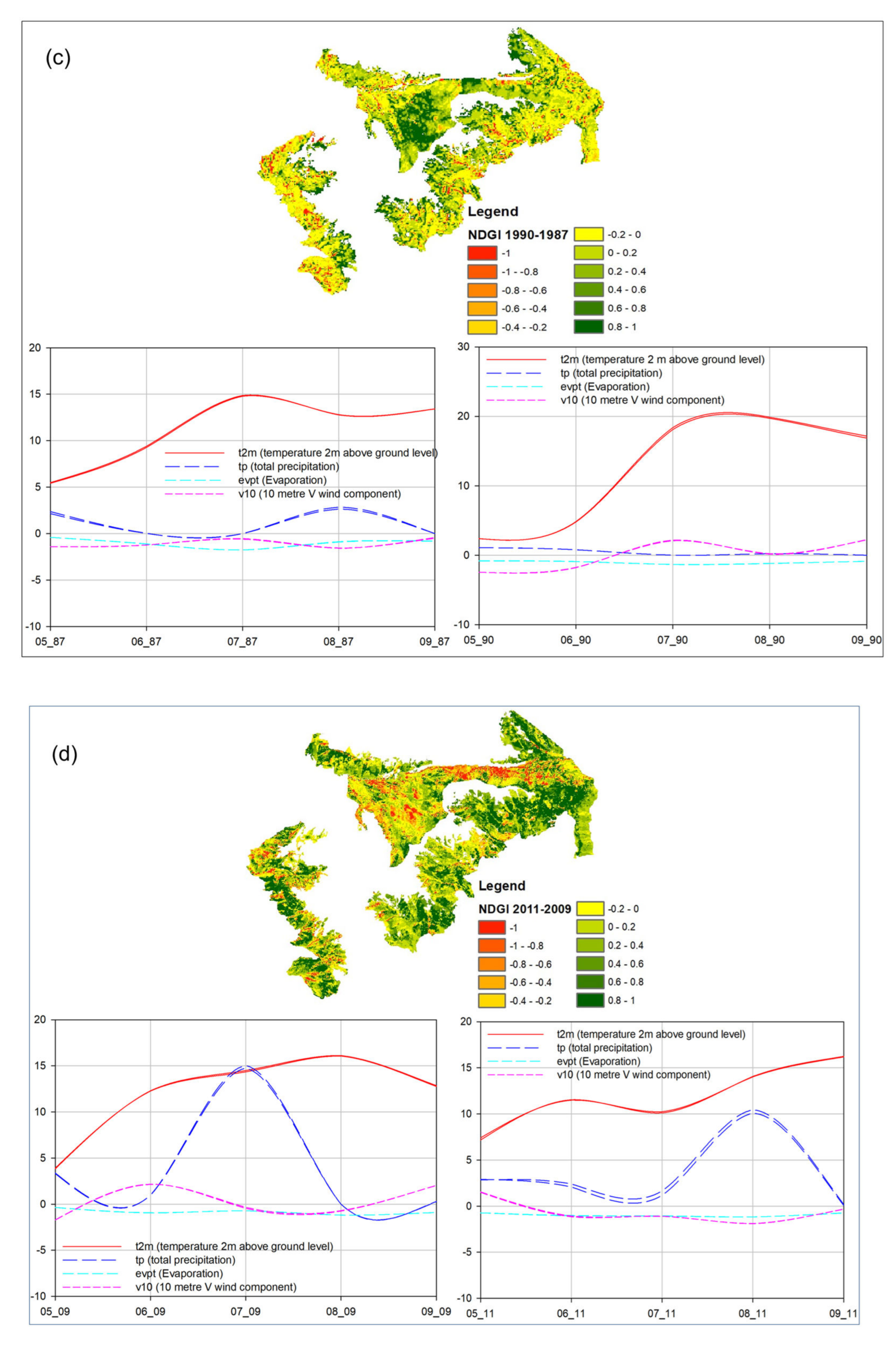
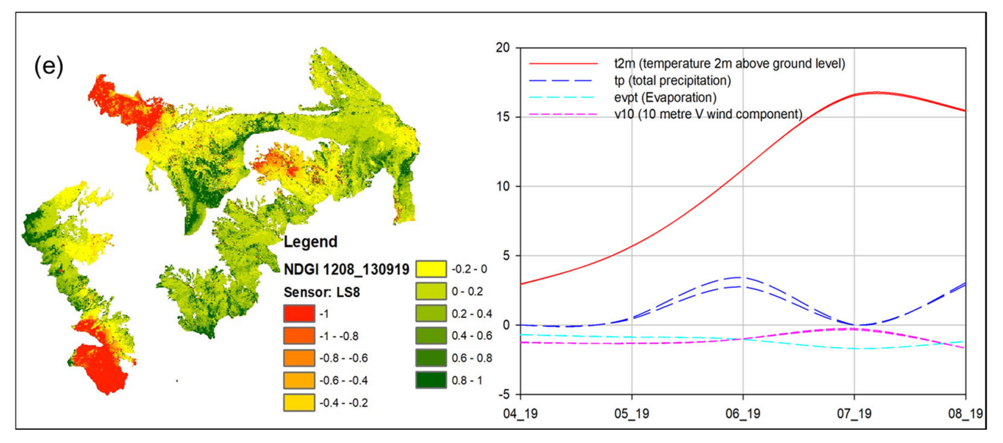
To improve the precision of change detection in the early Landsat images, we restore to the sensitive NDGI index [88]. NDGI is a valuable part of the remote sensing indices portfolio for different purposes, including crop monitoring [98,99], disturbance detection and response [100,101], flood detection [102], ecosystem risk assessment [28], wetland ecosystem services [103], etc. Earlier work [7,90] proves its usefulness for evaluating shorter time series of remote sensing images in this same study area. In this study, we use NDGI to cope with the lack of georeferenced historical data on ecosystem species composition. The earliest available spatial atlas [77] has very low resolution (1:600,000) and a description of communities that is very different from the current EU level and global classifications. Therefore, its usefulness concerning inferring the semantic and ontological compatibility is only limited to ecosystem type and does not allow for tracking subtler changes in ecosystem conditions or species composition. In a first analytical step, we analyzed the NDGI TMs together with climate data (Figure 8) to identify the climatic constraints to vegetation growth (such as extreme temperatures or insufficient precipitation). The resulting scenes are useful both for observing the ecosystem conditions’ dependence on climate and local environmental factors influencing microclimate (in particular elevation), and for determining changes in spatial distribution/exploring species composition, as detailed below.
As an additional analytical step, the generated NDGI TMs also proved useful for detecting outliers and eliminating problematic satellite scenes such as the image derived on 13 September 2019, which we identified through co-analyzing the NDGI TM between 13 June 2009 and 16 September 2019 and climate data. The reasoning behind this process is detailed in the Supplementary Materials, Section S5.
(4)
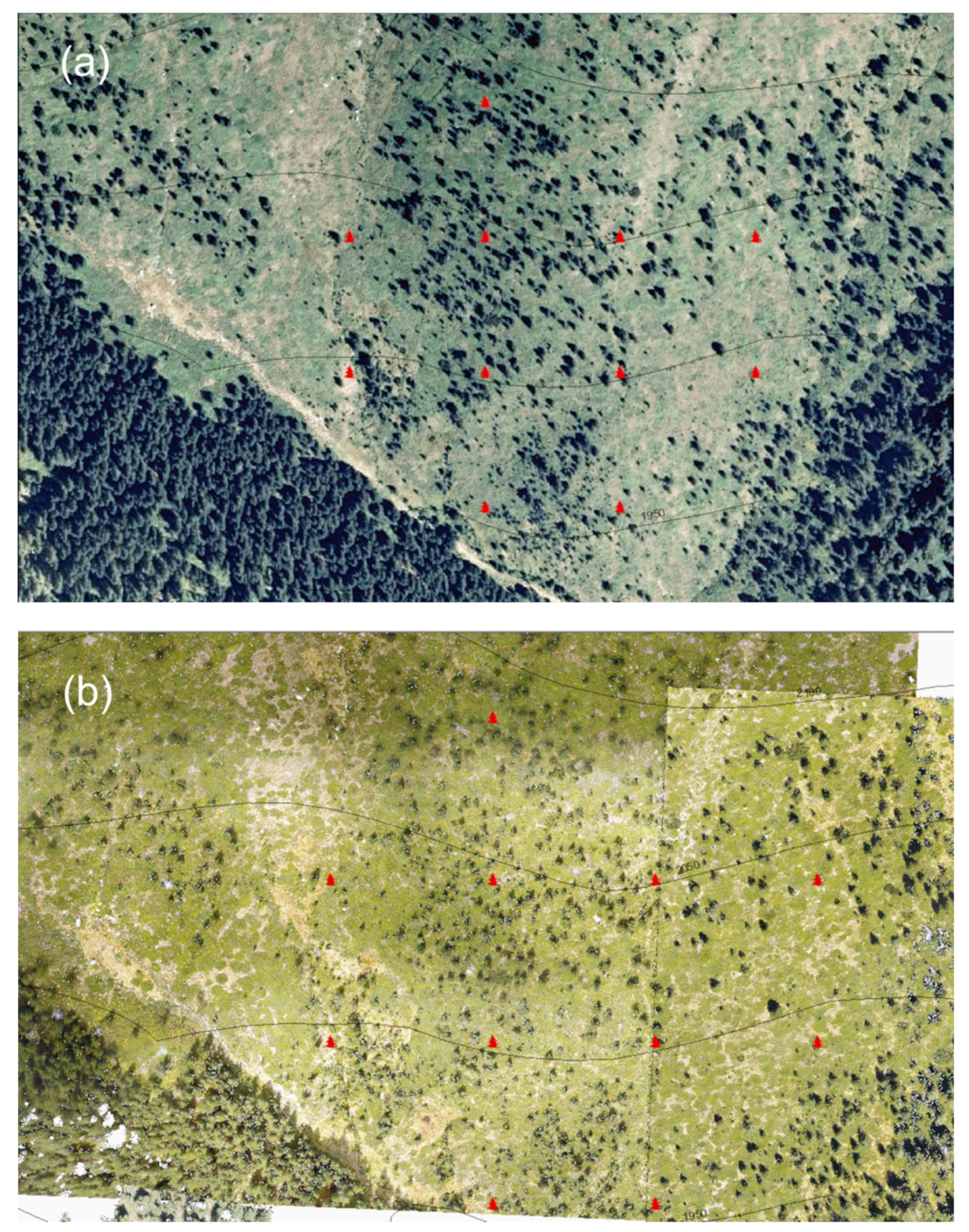
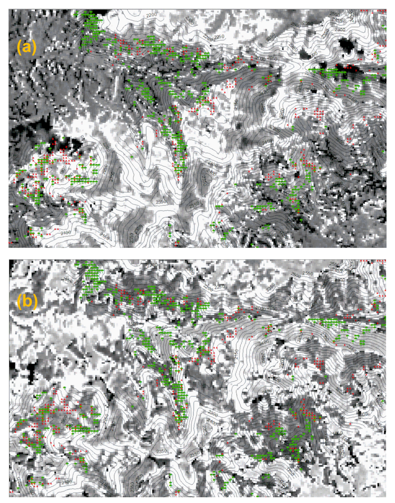
The lack of a long time series for tracking changes in spatial extent of the ecosystems within the landscape is a particularly challenging case for data fusion. This is so partially due to the coarser resolution of early satellite imagery that increases the uncertainty in detecting succession, and partly due to the changing signal within the same ecosystem type caused by changes in species composition, local microclimate, etc., which prevents geospatial reasoning on ecosystem extent based on single satellite scenes. At the same time, our data does not cover full vegetation seasons to enable reliable location of vegetation types by phenology. The most convenient data sources on ecosystem extent among the available data are the Copernicus High Resolution Layer (HRL)—new products currently only available with the information needed for our analysis in two baseline years, 2015 and 2018. Such a short “timeline” of two points is by itself insufficient for exploring trends in the change of ecosystem extent, being at most sufficient to specify the current extent and approximate species composition of ecosystems. Observing long-term changes in extent therefore requires creating a semantic link to data not directly attributable to extent. Such semantic linking allows, in effect, for performing reanalysis of multiple, various scale data sources for extent and condition. In the case of succession, the semantic inference that enables reanalysis back in time includes detecting the earliest signals of active growth in locations with proven later changes in ecosystem extent detected at the end of the period. In this manner we can use, information on the ecosystem type, location and first detection of the vigorous new growth to approximately date the beginning of the succession. Such an approach also has its limitations since it only applies to clearly defined and spatially stable ecosystems (deciduous and coniferous forests, heathland and shrubs). It is therefore not applicable to ecosystems with features less discernible through remote sensing (in our study area: Grasslands, water ecosystems). The data reanalysis consists of locating stable features detected at the end of the period and locating the earliest available signals for the forming of these features. To cross-check the changes in ecosystem extent, we compared the resulting change maps from the Copernicus Grassland HRL to the corresponding decline in grassland extent, and cross-validated the findings with earlier ortho-photo, our own drone imagery and the forestry database. Figure 9 shows representative spots of cross-checking the spatial extent. Targeted collection of dendrochronological information through ground studies in the identified spots could provide for further reduction of uncertainties, better dating and ground-truthing to form datasets for machine learning or AI applications.
For the purpose of species composition data reanalysis, semantic inference on the change in species composition includes locating places of known changes in the ecosystem composition in Copernicus HRL between 2015 and 2018 (in our case—spread of broadleaved species within coniferous forests) and observing the vegetation indices back in time to date the beginning of this process. The process is illustrated for representative parts of our study area in Figure 10.
In this manner, the fusion of different data sources can form a longer quasi time series of heterogeneous data sources on extent and condition. In our case, the composite data series covers the period 1987–2018 and includes the earliest Landsat 1–3 missions at the beginning of the period (images of 80 m pixel in two spectral bands); orto-photo and terrestrial data for the 2011–2016 period; and Copernicus HRL (100 m pixel) grassland and tree cover density products for the base years 2015 and 2018.

3. Results

3.1. Results of the Remote Sensing Data Processing

3.1.1. Remote Sensing of Spatial Extent and Distribution Trends

The cross-verification of the expert products together with forest database data shows a high degree of correlation between the datasets (see Figure 11). The available HRL products for grassland and forest ecosystems (which comprise most of the landscape mosaic) are presently insufficient to form a timeline of only two data points for three years. However, as detailed in Section 2.3.4, data fusion and re-analysis allows for forming a longer timeline of different but semantically compatible datasets. In particular, the co-analysis with NDGI for earlier satellite scenes and climate data (correlations can be seen in Table S5 of the Supplementary Materials) supports our second hypothesis about climate change-induced ecosystem dynamics. This is so since the remaining abiotic parameters are largely unchanged, while anthropogenic activity was traditionally weaker and extensive in most of the inaccessible parts of the study area and has ceased completely since its inclusion in the Natura 2000 protected areas network. The comparison of spatial trends shows upward expansion of both broadleaved and coniferous forests—with broadleaved expansion occurring as high as 2000–2100 m—and decline in grassland ecosystems’ extent in the lower elevations bordering the forest. Figure 11 presents the results of data reanalysis and fusion across the entire study area. The upward extension found by joint analysis of Copernicus HRL and the forest database is confirmed and dated more precisely by extending the data series back in time through NDGI between selected satellite scenes. The fused data further reveal that southern slopes are more conductive to accelerated growth of broadleaved species, whereas accelerated upward expansion of coniferous species is more frequent on the northern slopes. This finding is important for focusing future field monitoring and dendrochronological verification.
The available ground data also support the observation on the transition from coniferous to deciduous forests due to climate change. In addition to our spatial analysis, all 24 polygons assigned to coppices in the forestry database are marked as “forest in transition” in the “forest type” field, some having been earlier classified as “rock” or “non-afforestable”. After disturbances, four polygons underwent transition to habitat 9130—Asperulo-Fagetum beech forests.
We observe the same general dynamics across the study area when analyzing the earlier vegetation growth through NDGI (see Figure S18 in the Supplementary Materials). The only negative NDGI values we observed are in the comparison of August 1977 and May 1984. They are attributable to the earlier stage of seasonal vegetation growth in the second scene.
The greatest difference in the NDGI TMS comparing scenes taken in the same stage of vegetation growth (between July 1987 and July 1990, and between June 1985 and June 1994) is noticeable in higher altitudes, both in coniferous forests and shrubs. There are areas showing growth trends despite the seasonal difference in temperature and precipitation in the two years (coppices, broadleaf deciduous forests, coniferous forests in lower altitudes). They contain faster growing vegetation that has net biomass gain and builds up carbon depots in the seven years between scenes, whereas grasslands’ small positive and negative NDGI numbers point to a relatively stable state or decline.
Both NDGI TMs between July 1987 and July 1990, and between June 1985 and June 1994 demonstrate the importance of temperature differences for the vegetation growth, especially in higher-altitude coniferous forests and shrubs containing coniferous trees. With most of the parameters being similar, both the rise in temperature between 1987 and 1990 and the earlier onset of higher temperatures seem to have a positive influence on all ecosystem types in the higher altitudes. Almost lacking precipitation appears to be the limiting factor on growth for all ecosystem types in the lower altitudes. The earlier onset of higher temperatures has an even more marked effect in June (comparison between 1985 and 1994) even though the temperature differences themselves are minimal and 1985 was a year with higher precipitation at the beginning of the vegetation season.

3.1.2. Condition and Functional Dynamics of the HME—Vegetation Indices (VI) and Climate Data Co-Analysis

Following the reanalysis of combined climate and vegetation indices data, we found correlations between NDGI that indicate patterns of active vegetation growth between two satellite scenes to be much stronger when calculated at the observation object’s characteristic scale. This is illustrated in Figure 12, which compares potential determinants of growth for each characteristic area of rapid coniferous and broadleaf growth (as identified by the changes in extent towards the end of the period) with the much more heterogeneous and large scale study area as a whole. In both focal areas, the correlation between ecosystem type and overall seasonal growth indicated by the NDGI signal is stronger than the same type of correlation in the entire study area (Figure 12b,c).
In addition, both in areas with broadleaf and coniferous expansion, the seasonal growth strengthens between earlier and later NDGI scenes as the expanding species grow in their new location, indicating their role as driver of overall growth (Figure 12b).
At the same time, the strong positive correlation of coniferous growth and elevation in coniferous expansion areas on a year-to-year basis between 1987 and 1990 (Figure 12c) is in line with the observed upward shift in ecosystem extent and emergence of succession in former grassland areas. The relatively strong negative correlation between dominant coniferous species and the expanding broadleaf species in the same year is in line with the change in species composition from coniferous towards mixed forest.
Annual climate differences, however, can significantly influence the year-to-year growth patterns, as shown in the NDGI comparison between early seasons of 1985 and 1994 (Figure 12c). While ERA Interim’s scale is much greater than the two focus areas, it informs the understanding of observed NDGI correlation anomalies. The climate modelling shows that 1994 had virtually no precipitation in June, whereas in 1985 the peak precipitation was in June (Figure S18c–e). As a result, the much weaker growth for 1994 in the more water-deprived higher plots of coniferous forest translates to a negative correlation between year-on-year growth and elevation (and to smaller extent, aspect). A slower upward expansion of broadleaf species is also observed in the less water deprived broadleaf focus area where the dominant coniferous species have grown much stronger than the expanding broadleaf species (as evidenced by the positive correlation between the coniferous dominated ecosystem type and NDGI in the 1985–1994 scene).
Positive NDVI values prevailed throughout the study period, which indicates good conditions with the HMEs. NDVI values vary according to the phenological stage within the vegetation period; we found that they correspond to the changes of t2m parameter, which confirms the correlation between t2m and NDVI established by a number of authors—Wang et al. (2003) [97], Pavlova and Nedkov (2005) [94], Katrandzhiev (2018) [90] and Katrandzhiev and Bratanova-Doncheva (2019) [7]. The seasonal dynamics of NDVI is most obvious in the last 3D graphic (Figure S6f) which presents the dynamics of NDVI changes in 2019. At the beginning of the VP (24 April 2019) when t2m values varied within 4 °C (see Figure 9) NDVI values were negative and close to 0 due to the presence of snow cover (Figure S16a). In the middle of the VP (03 July 2019) when the t2m varied within 16.5 °C high values of the NDVI were observed (0.5–1), i.e., the amount of the leaf biomass increased and the functioning of the vegetation cover became more active. At the end of the VP (Figure S17b,e,h,j) we observe decreased NDVI values, suggesting decreased values of the t2m parameter. This confirms the expected influence of temperature on NDVI.
We assessed the selected HME condition by means of NDVI calculation based on a set of satellite data and the influence of the t2m parameter on the NDVI. We verified the results via NDWI and NDGI calculations (Figures S7–S18)
Snow cover is one of the major distorting factors in analyzing time series of vegetation indices from satellite imagery during the vegetation period, appearing as late as May/June and as early as October (Figures S7c, S8d, S14a,i, S15a and S16a in the Supplementary Materials).
Close to the beginning of the VP, the seasonal fluctuations in temperature and precipitation seem to have a strong influence on the intensity of vegetation growth. The snow in April and early May in Figures S14b,j, S15b and S16b had less impact on vegetation growth farther down from the ridge than the snow in late May at the beginning of the time series (Figures S7d and S8e). This finding corresponds to the trend of rising temperatures over the period, as well as a steepening of the temperature curves in the 1990s. It suggests that the lengthening of the vegetation season in September contributes to increasing the HME’s resilience to cold spells occurring at the beginning of the vegetation season, with overall conditions remaining good despite the seasonal shift. This proves that resilient ecosystems can better mitigate climate stress.
The presence of snow in remote sensing imagery corresponds to low values of t2m from the climate model, thus proving the value of fusing these two types of data despite the lack of sufficient spatial resolution in the climate model. Temperatures vary between 6 °C in May 1984 and up to 8 °C in May 2017, and the NDVI values are correspondingly low (0–0.2 for the alpine shrub and grass vegetation, 0.2–0.4 in conifer forests and above 0.5 in the broadleaf and coppice stands in May). As a reference, NDVI is almost uniform 0.2–0.4 in most ecosystems and 0–0.2 in the shrubs closest to the snow cover. This finding confirms the usefulness of cross-referencing between the remote sensing data and climate model.
There is strong seasonal dynamics during the growing season, with similar growth patterns in June and July for all ecosystem types except the broadleaf deciduous forests: Growth has not reached its maximum and its speed distribution appears to be mostly dependent on the altitude and not so much on the ecosystem type. The leaf biomass of broadleaved deciduous forests grows faster than all other ecosystem types. At the beginning of the available observations, NDVI is in the range 0–0.2 for the alpine shrub and grass vegetation, 0.2–0.4 in conifer forests and above 0.5 in the broadleaf and coppice stands. In this period, whenever precipitation is not a constraining factor, the intensity of leaf biomass growth appears to best correlate with temperature (and grow as the temperature rises and the vegetation season possibly lengthens). This progression is visible in Figures S9b,e, S10b, S11b,f and S13e,h,k. At the end of the period, the NDVI values increased (0.6–0.8) in the dominant conifer forests in unison with the rise in temperature (~12 °C in June 2019, Figure S16g in the Supplementary materials).
The vegetation growth peaks in August and September, as seen in the higher NDVI values in the late summer thematic maps. Apart from 1977 which has low NDVI values in most ecosystems, the index varies between 0.4 and 0.6 in most territories in the study area in 1985 (Figure S8b) and between 0.4 and 0.6 for shrubs, 0.6 and 0.8 for the dominant forests and up to 1 for deciduous forests in 2019, confirming the increase in forest biomass production and carbon sequestration with warming climate.
At the end of the VP, the prevailing NDVI values vary from 0.2 to 0.4 in the higher parts and 0.4 to 0.6 in the lower part of the study area in the first available scene from October 1986 (Figure S8e,h). With growing temperatures, vegetation is more active in October with slowdown mostly in the shrubs at the highest elevation, as evidenced in the two scenes of Figure S15h,k.
Apart from these general trends, the second part of the study period displays a number of anomalies. In 1994, the climate model shows the lowest precipitation in the entire time series, causing a break in the early season growth pattern. There is a relation between the climate model showing almost no precipitation at the beginning of the vegetation season (Figure S10f), and the NDVI readings of a slow growth in the NDVI thematic map (Figure S10e). In comparison, low precipitation in September 1992 after the high precipitation in mid-season is still a limiting factor for high NDVI, but to a lesser extent (Figure S10b,c). We observed a similar albeit less acute water limitation in 2000. The years 2009, 2011, 2016 and 2018 show an unseasonal high precipitation peak preceded by too low precipitation in the beginning of the VP (Figures S12g,n, S13g and S15m). The frequency of such occurrences suggests that they may form a new trend in shifting precipitation patterns with climate change, which needs close monitoring in the coming years. However, the existence of such a trend is not certain since 2019 displayed a double peak in precipitation (Figure S17l)—a possible stress factor for the vegetation growth. While there appears to be corresponding fluctuations of NDVI readings within just one month in Figure S17b,e,h,j, we infer that one of the scenes in 2019 may be an outlier (see Section S5 in Supplementary Materials).
In observing these fluctuations, the cross-verification of NDVI with NDWI for the same scene has a growing importance. It can be used to explain spatial differentiation in growth patterns. For example, Figure S8f shows a correlation of growth patterns with NDVI in Figure S8e but also a correlation with the climate model in Figure S8i since the precipitation modeled for early June (Figure S8c) is still visible as evaporating water reserve in the snow on the ridge. Where available, NDWI also demonstrates the spatial distribution of water content in the foliage at a much more fine-grained scale than the climate model’s precipitation component (Figure S11d). In combination with NDVI and climate modeling, it can help verify time lags between precipitation and changes in vegetation growth. An example of such verification is the overall correlation of timing between high NDWI and precipitation fluctuations; e.g., the June 2009 simultaneous dip in NDWI and precipitation was followed by increased precipitation and a delayed recovery in July 2009; the opposite correlation of peak precipitation, growth and leaf water content occurred in August 2011—see Figure S12. NDWI is also prone to distortion by clouds (as shown in Figure S13d–f), and to avoid misconstruing the simultaneous dip in NDVI and NDWI as disturbance, there is a need to use improved cloud masks as these become available in newer remote sensing products, observing a longer time series over such spots or using ground measurements from meteorological stations. The usefulness of NDWI grows with the number of high quality satellite images available. For example, in 2018 the interplay of NDVI, NDWI and climate modeling shows the decrease of available water in parallel with vegetation growth in May. While there is almost no precipitation, the available moisture is absorbed by the vegetation and does not evaporate even after the rainfalls in August (Figure S15), indicating resilient ecosystem functioning. Similarly, better understanding the effect of the double dip in precipitation in 2019 is possible once we account for:
(a)
the using of water from melting snow in April (higher water content despite lacking precipitation—Figure S16a,c);
(b)
a slowdown of growth in August as the June rains are absorbed and no additional precipitation comes while the temperature keeps rising (Figure S17a,c), and
(c)
the second surge in growth in the second half of September with the new precipitation—see Figure S17d,f,j,k.
Based on the findings of this and the previous sections, we can find ecologically meaningful links between different datasets and can go beyond the statistical analysis, therefore confirming the first hypothesis on the utility of data fusion on the semantic and methodological levels and utilizing all available data.
We furthermore achieved a co-benefit of testing the hypothesis of data extensibility by developing corresponding candidate indicators that use remote sensing data sources and address a more integrated approach to ecosystem monitoring by widening the data sources used in it. These indicators are adapted for easy remote monitoring with a minimum of ground data, thus contributing towards the ongoing monitoring of changes in ecosystem extent and condition caused by climate change. We settled for proposing for future use two linked indicators describing the ecosystem dynamics related to extent and condition of HME that are sufficiently underpinned by existing data: “Habitat extent increase/reduction attributable to climate change”, and “Ecosystem succession attributable to climate change”. These two candidate indicators on ecosystem condition may, after verification, become part of the methodologies for terrestrial ecosystems (Table 2) and facilitate automated monitoring of climate change impacts on HME through remote sensing. Both candidate indicators aim at complementing the existing indicators in the methodologies of the respective ecosystems that form the landscape in our study area. Adding them to the Methodological Framework is important with a view to the scientifically established acceleration of climate change.
The proposed indicators require a quite rigorous approach to distinguishing between extent change and succession caused by climate change, and similar changes caused by other factors, notably grazing and land management that are identified as the main factor influencing the speed of changes in the HME grassland–forest ecotone [5,104,105]. Therefore, they are only suitable for forward-looking remote monitoring of the spatial ecosystem extent in our study area and other HMEs with a high degree of naturalness (reusing them in intensively managed HMEs would require additional research and their adaptation to account for human influence on the ecotone and species composition). While our study area has been protected with no large-scale anthropogenic influences since 1933, the data in [77] proves the existence of land management and grazing in the late 1980s. Therefore, we take the expansion of the NATURA 2000 network in Bulgaria (legislation adopted in 2007 and extended in 2008) as the moment in which these influences were legally suspended.
To avoid biases in the indicators, establishing the causes underlying the change in extent is important. At the same time, it would be difficult or even impossible by only looking at ecosystem information since there is a need to consider a time lag after the establishment of the legal protection status of NATURA 2000. Therefore, we verified the lack of disturbances in the ecosystem by other means available, including:
-
scientific publications and official documents: The orders determining the management regimes for the Parangalitsa reserve (in force during our entire study period) and NATURA 2000 protected areas for the rest of our study area (in force since 2007, extended in 2008)—both stipulating the seizing of economic activities;
-
georeferenced sources: Bondev [77] for the land use and management regimes in the 1980s as well as the subsidy eligibility layers for grassland management (since 2015);
-
agricultural data to confirm that the alpine and subalpine grasslands are largely undisturbed after this date and any occurring grazing is extensive (therefore, not significantly influencing the landscape).
In this context, the use of semantically consistent data fusion allows the deduction that the main driver of succession in this landscape since 2008 is climate change.
Based on the above, we can evaluate the parameters for the two candidate indicators only for periods of proven lack of anthropogenic disturbances for at least 8–10 years of undisturbed ecosystem development to ensure that the dynamics of ecosystem processes is exclusively attributable to climate change. This means that, in our study, only the latest part of the study timeframe is useful for deriving reference values for our candidate indicators—a minimum of 5 to 10 years without disturbance, that is from 2015 onwards for the entire study area.
We selected the reference values of the parameters measured to contain easily available but quality controlled remote sensing and expert products. In this manner, changes in data sources will be easily traceable through the metadata of the expert product versions and a reanalysis in the expert products performed by their publisher can be monitored and trigger a reanalysis of our indicators as well.
We estimate the initial values in Table 2 having in mind the observed speed of ecosystem change in Copernicus products produced for two base years, by ecosystem type. However, as more such products will become available in the form of continuous data series, these values will have to be reviewed and verified before including them in the Methodological Framework. The availability of new data or satellite products is very likely to prompt an adjustment of reference percentage values, especially for the proposed succession indicator (red in Table 2). We expect that with establishing the Long-Term Ecosystem Research site Parangalitsa (whose infrastructure development started in 2021), better ground data on biodiversity and abiotic heterogeneity will also become available over time and will be conductive in establishing the proper reference values for these candidate indicators.
Having in mind the observed dynamics in ecosystem condition (Section 3.1.2) and the observed NDVI values in our time series, we propose a new, functional parameter to complement the largely static IP index of the terrestrial ecosystems where a detailed field inventory is not possible (Table 3). A correlation analysis with the IP index calculated using the forest database or a future forest inventory will allow for finding outliers and reducing uncertainty, for a more robust remote monitoring of ecosystem conditions. In this manner, it can also semantically and ontologically connect the ecosystem condition and ecosystem service indicators in the methodologies.
This candidate indicator requires additional verification, including some or all of the following: Cross-verification with NDWI and climate data time series (temperature, precipitation); error correction via NDGI; field verification: Vegetation inventories and IP index if it becomes available for NATURA 2000. In addition, a more precise localization of heathland and shrubs is a prerequisite for determining the missing reference values for this ecosystem type since it has very few polygons in the forest database but according to the Copernicus HRL products is likely to be one of the most dynamically developing ecosystem types.

3.2. Analysis of Climate Parameters and Cross-Validation with Vegetation Indices

We analyzed the climate parameters ‘t2m’ (temperature 2 m above ground level), ‘tp’ (total precipitations), ‘evpt’ (evaporation) and ‘v10’ (10 m V wind component) (Table S5 in the Supplementary Materials) and plotted graphics of their dynamics for the entire period of available ERA Interim data (40 years) within the vegetation periods (VP). Based on the results by climate parameter, we could establish a trend of increasing values of the t2m parameter during the months May–July and September for the full 40-year period. Only for August, we found a trend of decreasing t2m values (Figure S3 in Supplementary Materials).
In order to test if there is an acceleration in climate change, we divided the 40-year period of ERA Interim data into two shorter periods: (1) 1979–1999 and (2) 1999–2019 (except for September parameters that are not available for 2019 in ERA Interim and therefore end in 2018). In each half period, we calculated the mean values of t2m given the minimal and maximal values for each month within the VP (Table S5 in Supplementary Materials). We observe trends of increasing mean temperatures in May–July and September during the studied period. In the second period, we observed increased mean values of the t2m parameter compared to the first period—for May by 2.2 °C, June by 1.1 °C, July by 0.9 °C and September by 1.2 °C. The only exception is August when we observe a trend towards decrease in the mean values of t2m by 0.6 °C for the study period (Table S6 in Supplementary Materials). We carried out Pearson correlation analysis between the NDVI and the t2m parameter in the study area which revealed sufficiently strong correlation between these variables (correlation coefficient- R2 = 0.605). The correlation table for this analysis is available in Table S5 in the Supplementary Materials.
The review and analysis of the annual climate plots reveal that, apart from the overall rise in t2m, high temperatures occur about a month earlier at the end of the period as compared to 1977, 1984 and 1985, suggesting a lengthening of the vegetation period. Confirmation by studying even longer-term observations and/or the new Copernicus Phenology HRL product when it becomes available for our study area appears necessary to confirm this conclusion as it may provide insights into the drivers of vegetation change.
Based on regression analyses and temporal dynamics analysis (Figures S1 and S2), we establish trends of tp decline in May (Figure S2a) and June (Figure S2b) within the studied period. In addition, we observe trends of tp increase in July (Figure S2c), August (Figure S2d) and September (Figure S2e) for the same period within the study area. In order to test the existence of a relationship between the NDVI and tp, we conducted Pearson correlation analysis (Table S5) between them in the study area. We found R2 = 0.0228 and p = 0.907 (i.e., p > 0.050). We established negative correlations for both NDVI–evpt and NDVI–v10, with correlation coefficients −0.275 and −0.0184, respectively. Therefore, we did not find definite trends of influence of the evpt and v10 in the NDVI. The findings of Section 3.1.1, however, suggest that such trends may well exist in some parts of the study area where other abiotic factors influence a strong dynamic of the ecosystem development/succession.
In Figures S4 and S5, we present the change dynamics of these parameters. When compared to the changes in the NDVI values throughout the study period, we were not able to establish a connection. Therefore, in the current study we establish that cross-analyzing the influence of the t2m parameter on the NDVI and HME conditions yields the best results as it is the only parameter showing strong correlation to the NDVI (R2 = 0.605).
This semi-qualitative analysis is in line with the complicated interplay of environmental factors that limit vegetation growth in different parts of the vegetation season; climate parameters are only part of these factors. Among climate variables, temperature seems to be the most obvious overall limitation to vegetation growth, while other parameters may influence it in different years without a clear trend.
We performed correlation analysis of NDGI and local parameters from the forestry database using the corrplot library in R (Figure S19 of the Supplementary Materials). The overall weak correlations between any two parameters taken across the whole study area is ecologically meaningful since it confirms the complex interrelations between growth and microclimatic environmental parameters, in line with the findings of Section 3.1.1 about the microclimate’s importance. It also reveals a scale mismatch for some of the possible correlations as they likely occur only in parts of our study area, as suggested by the data fusion reanalysis in Section 2.3.4. On the current scale of observation, the higher correlations would exist only in areas where favorable microclimatic conditions influence the vegetation dynamics, whereas large areas with relatively homogeneous microclimate or vegetation or weaker changes in vegetation growth (typically alpine grasslands or shrubs) yield weaker signals and therefore weaken the overall correlation. This is visible in Figure S19b, where the strongest observed correlations are to parameters determining the microclimate—elevation and slope. In contrast, strong climate fluctuations lessen the impact of local microclimate—see Figure S19c for year-to-year comparison and Figure S19c for the seasonal comparison. As such, the sensitive NDGI must be used at smaller scale for cross-validation of both NDVI and NDWI.
As to the nature of microclimatic determinants, the spatial analysis of Figure 9 strongly suggests the need for more detailed, field-measured climate data in focal points of particularly dynamic ecosystem change, specifically the southern facing slopes in the higher altitudes and the forest—alpine grassland ecotone, especially in locations with established succession. Such targeted data collection would enable a georeferenced and hopefully much more precise correlation analysis.

4. Discussion

The present study in some of its parts repeats the methodology of earlier work of some of the authors in the same study area [7]. However, it is much wider in terms of data integration and consistent application of the Whole System approach. To our knowledge, this is the first study that makes use of the ontological and semantical power of structured indicator–parameter systems as defined in the Bulgarian Methodological Framework [26] and, in this sense, also contributes to the worldwide research on the Whole System application. A summary of the results follows in this part.

4.1. Methodological Results

With a view to ontological similarity defining one-to-many relations between ecosystems and habitats, forestry data and our field verification (Section 2.3.4), we were able to narrow down the ontological similarity on level 3 (ecosystem subtype to habitat) for the forest ecosystems in the study area by verifying the types of habitats occurring in the forest ecosystems (Figure 7, middle). Due to insufficiently granular data about the other ecosystem types, we were only able to verify the level 2 relation for the other ecosystems present.

4.2. Hypothesis Verification

Our study confirms both the working hypotheses we presented in the introduction. In support of our first hypothesis:
  • We confirm the semantic consistency of the Methodological Framework by using new data sources in a manner consistent with the Whole System approach. Based on this work, we propose an ecologically meaningful extension by adding a candidate indicator set on climate change impact. These indicators are of particular importance for the sensitive HME. They are balanced on a landscape level and reflect the trade-offs between the extent and condition of different ecosystems in the course of climate change-induced succession since in the limited habitat the expansion of one ecosystem type is at the expense of another. In addition, we explore the scale of observation and confirm its importance in reducing uncertainty when a dataset’s scale (in our case, ERA Interim) significantly exceeds the characteristic scale of the object of observation.
  • We use an ontologically consistent approach to utilize data collected for different purposes (in this case use habitat data) for verification of a Level 3 crosswalk for forest ecosystems. In addition, through this crosswalk field data on habitats can be useful in conjunction with vegetation indices for a future remote monitoring of forest areas where the dominant vegetation type consists of climate-vulnerable species. This allows for focusing our limited fieldwork resources on problem spots.
  • The production pipeline of Copernicus remote sensing products delivered by the European Environment Agency utilizes significant human and financial resources to ensure their methodological consistency within a single information infrastructure; they also undergo rigorous quality checking and control of both data and metadata. Incorporating them in a future remote monitoring within the Bulgarian Methodological Framework would therefore add to the strong methodological and information-technical consistency of the Whole System approach with very low additional costs for exploring data poor biodiversity hotspots like our study area. This seamless incorporation of a new data source as a basis for new candidate indicators further confirms the extensibility clause of our first hypothesis. Data fusion and co-analysis form the basis to confirm the possibility to derive ecologically meaningful information from all available data sources.
  • We use data fusion also to cross-check and verify data sources, thus reducing uncertainty and supporting our hypothesis that applying the Whole System approach allows for more reliable data integration. In the course of our research, we confirm the suitability of the selection of vegetation indices and their combination with expert remote sensing products, climate models, publications or other non-georeferenced documents and field data as a set of mutually complementary data sources that allows confirming synergies and identifying outliers.
  • Beyond the expected results, we further found that using data integration:
    allows the additive introduction and use of a higher number of very diverse data sources for a more reliable monitoring of both the ecosystem extent and conditions in data sparse environments;
    supports finding the appropriate observation scale for different scientific questions; and
    enables extending the holistic approach of the Methodological Framework to accommodate for future ecologically meaningful linking of ecosystem condition and ecosystem services in the sense of natural capital accounting principles that can replace their current assessment within the Methodological Framework. This, in turn, underpins the use of the Whole System approach in a socio-ecological context.
The analysis of fused data also supports our second hypothesis. We were able to observe the impact of climate change on both ecosystem conditions and functioning, and the landscape level changes in the spatial distribution of different ecosystems and the species composition. Based on the conceptual and instrumental advantages of the Whole System approach, the selected toolbox allows for complex monitoring that goes beyond the observation of species, ecotones or single ecosystems.
In terms of ecosystem extent, our study suggests that climate change may influence the ecosystem succession. A longer time series may confirm an acceleration as suggested by NDGI observations of early succession signals in the 1990s and the more rigorous recent changes found in Copernicus HRL data. In such cases, regular ecosystem extent monitoring may identify the possible approaching of tipping points in extent reduction or species composition for some ecosystems. For the grassland ecosystems in our study area, such speeding decline may also influence the overall ecosystem resilience and reduce the habitat of endemic species. Should the observation of a longer time series confirm such accelerating trends, the observation frequency for some ecosystem types might also need reconsidering in the Monitoring Guide [76] of the Methodological Framework.
On ecosystem condition and functioning, we made a number of observations.
We established the correlation between vegetation indices and the changes of selected climate parameters (temperature, t2m; total precipitation, tp; evaporation, evpt; and 10 m V wind component, v10) throughout the 40-year period—from 1979 to 2019—within the study area. We found an overall increase in the t2m parameter during the vegetation period between the start and end years of observation; with the exception of August the values of the t2m decrease. In addition, based on the regression analysis, we found an overall increase of the tp parameter. These trends suggest that climate change challenges the resilience of HME ecosystems, which are increasingly subject to dryer and hotter weather during the vegetation peak seasons. At the same time, lengthening the vegetation season contributes to increase in biomass production and overall resilience. Seasonal shift in phenology is important to observe closely, as revealed by the NDGI correlation analysis (Section S5 in Supplementary Materials).
With regard to the forests, we could not establish conclusive long-term links between tp, evpt and v10 parameter change and the NDVI changes over the entire study area. The results of detailed analysis in different years suggest that the limiting factor to growth changes depending on the combination of climatic variables and can be precipitation (years 1994, 2000) or temperature (years 1986, 2009). The only direct connection and dependence we were able to confirm is the connection between the t2m parameter and NDVI. Overall, the interplay and combined influence of both the t2m and tp on the NDVI across the study area confirms the findings of previous studies.
At the same time, the spatial analysis of species change patterns in the forest parts of our study area suggest the importance of microclimatic parameters, in particular elevation and slope. This finding points out the need for meteorological ground data and smaller scale data fusion to verify the importance of these factors in the conditions of climate change.
We observed seasonal and annual dynamics arising from these interrelations in the NDVI value distribution in the main ecosystem types and forest ecosystem subtypes, forming the composition of the studied HME. The increasing temperature and total precipitation in the last two decades appear to have led to an increase in the NDVI values, suggesting an improvement in the vegetation functioning and conditions through the last 20 years, as well as changes in species composition accompanied by growth acceleration. The subalpine and alpine grassland and shrub ecosystems may be more susceptible to climate parameter changes compared to the forest ecosystems. Since grassland ecosystem dynamics develop at a higher speed, the collection of time series for these sensitive ecosystems is necessary to facilitate better remote monitoring. On a subtype level, conifer forest ecosystems show resilience to changes in climate parameters and remain functionally stable; there is also a trend of succession towards higher altitudes. The more vigorous vegetation process that we observed in the broadleaf and coppice forests is an indication of future changes in their distribution to higher habitats atypical for them, thus influencing the species composition. We furthermore found indications that the changes in climate parameters led to a longer vegetation season, most clearly seen in 2019. Future phenological observations and analyses are necessary to confirm and specify these trends.
By introducing a rigorous approach to extent and condition observations, our study also creates a basis for further research on the HME’s capacity to provide ecosystem services related to the primary production ecosystem function along with the new UN System of Environment Economic Accounting (SEEA) standard. Further analyses based on a combination of field observations of the energy budget and remote sensing are necessary to specify and assess the dynamics of these ecosystem services. A more detailed study of some key services such as pollination will also require additional holistic methods such as pollinator efficiency studies [106,107,108], observation of environmental stress [109] or eDNA [110,111] to establish a better overview of species composition and within our large study area.
The evaluation of vegetation indices confirms the resilience of the HME ecosystems, whereas the spatial analysis using HRL products demonstrates spatial changes at the landscape level. Since the study area is protected and human intervention is minimal, we expect that climate change will remain the main driver for most of the developments in quickly developing ecosystems (grassland, sparsely vegetated areas). As tree growth is much slower than the retreat of grasslands, we expect these ecosystems’ dynamic to benefit from increased observation frequency enabled by the better availability of remote sensing imagery. While both forest and grassland ecosystems show increasing growth dynamics as climate change accelerates (as confirmed by joint analysis of the Copernicus HRL products for the end of our observation period), the relatively late appointment of NATURA 2000 protection for all of our study area means that both succession and change in species composition started before its full protection. Therefore, we cannot fully attribute the succession in the tree line ecotone to climate change for the period 1990–2015. Nonetheless, we can conclude that:
  • Observing the gaps between the Copernicus Grassland and Tree Cover Density HRL products is a good way to localize succession areas of particular monitoring interest for both future fieldwork and observation of the newly formulated extent and condition candidate indicators for climate change impact;
  • The use of new remote sensing products will allow for a finer grained monitoring. This, in turn, would enable downscaled monitoring, the early identification of potential tipping points and problematic areas resulting from climate change-induced disturbances such as storms, hails or pests. Such upcoming potentially useful new products to add to our remote sensing portfolio are the small woody features for remote localization of heathland and shrub ecosystems and phenology for better tracing the effects of climate change on the ecosystem.
  • Changes in forest ecosystems are slower but still observable over longer timescales. Due to the slower processes in forests, both the impact of earlier anthropogenic activity and the results of natural disasters are of stronger local influence. As they require more accurate and frequent observation, the introduction of Synthetic Apreture Radar (SAR) products for monitoring in cloudy days and the upcoming launch of hyperspectral Copernicus missions are prospective important directions for enhancing the remote sensing parameter portfolio of the Methodological Framework.
  • Together, these directions will largely enhance the toolbox available for the monitoring of climate change effects on HME. They will be better suited to inform and support:
  • future directions for targeted fieldwork,
  • scientific products delivered through the European Long-Term Ecosystem Research Network, and
  • the implementation of national and regional climate change adaptation policies.

5. Conclusions

The current paper presents, for the first time in a Bulgarian high-mountain ecosystem, a Whole System approach to long-term (42-year period) assessment of the response of the worldwide sensitive HME ecosystems to changes in climate parameters. We demonstrate the usefulness of a toolset of complementary approaches: Selected indices from satellite-derived data (NDVI was verified by the NDWI and the NDGI), HRL products and cross-validation with climate modeling data and ground observations/inventories as an integral part of the Whole System approach.
Studying long time series also presents a number of challenges and uncertainties. In our study area; these consisted in:
Technical constraints of the sensors used in the earlier years. Since missions of different space agencies overlap, the granularity of available imagery varies with the imaging satellite’s sensors, sometimes even within the same year or month. Thus, a source of uncertainty is the need to intercallibrate data series, e.g., between different Landsat sensors and Sentinel—which is only partially alleviated by the use of NDGI.
Uniform and precise climate modeling is not available for the first years of our study period. The ERA Interim data series started in 1985 and was discontinued in August 2019; the replacing dataset ERA 5 was not available for the entire period at the time of data processing. Using ERA 5 in later studies requires careful cross-checking of available data and identifying (where possible—also assessing) the cross-calibration uncertainties and errors.
A dearth of suitable satellite images due to the shorter vegetation season and the frequent occurrence of clouds. Therefore, our dataset is imbalanced towards the last years when Landsat was complemented by Sentinel imagery and both the frequency and quality of available image data, as well as the number of vegetation indices retrievable from the new sensors, increased.
Uncertainty of data in the forestry database. The existing forestry database has no QA information either in the published official data collection guidelines or in the dataset itself. Furthermore, the relatively limited data on species composition suggests limitations in the scope of field surveys over the years.
We found significant data and research bias towards studying forest ecosystems and, consequently, could not perform the same quality analysis on the grassland, shrubs and sparsely vegetated ecosystems in the study area. To be able to repeat the study uniformly within the entire area of interest, a more detailed mapping, aimed at filling the spatial gaps on an extended study area (yellow colored parts from the outline in Figure 1), would be necessary.
The great scale disparity of data sources at the appropriate observation scale for our study object limits the current climate data fusion approach to semi-qualitative observations.
All of the above, along with the incorporation of new remote sensing products as specified in the Discussion section above, presents a number of instrumental research directions to improve the methodology of our study as new methods and products become available.
At the same time, this toolbox of complementary methods allows for specifying new ecological research questions that present a wide field for future work:
Exploring a denser time series of satellite imagery and the corresponding ERA 5 climate parameters along with field data would be conductive to determining the best time slots for reliably identifying ecosystem types and subtypes depending on the best correlations with other environmental factors during the vegetation period.
Data fusion involving climate models requires additional research in finding the appropriate observation scales of complementary ground and remote sensing data.
The joint analysis also allows for hypothesizing on a shift in the extent and upper border of the forest ecotone, as evidenced by the surge in the vegetation growth of shrubs (containing coniferous trees) located in the highest parts of the study area. Another key direction, therefore, is the regular observation of phenology shifts and seasonal differences between the reflectance of ecosystem types/subtypes, with broadleaf forests being easiest to spot remotely within the vegetation season.
Focused dendrochronological studies, in areas where persistent changes in ecosystem extent, conditions or species composition are detected, are necessary to support the automation of monitoring through machine learning and AI.
Due to the sensitivity of NDGI, a correlation between the NDVI variation and disturbances (e.g., windthorows) in much smaller spots as described by Panayotov [81] in some parts of our study area could be the object of further research.
With a view to the delay in mapping and assessment of ecosystems within Natura 2000, another important research direction is the field verification and detailed mapping of the location of ecosystems other than forest, by incorporating a wider toolset of field methods such as the ones mentioned in the Discussion section above.
The assessment of the provisioning capacity for ecosystem services related to the biomass is likely to become easier as more and better quality remote sensing imagery becomes available in conjunction with field data using new standard observation methods.
The use of climatologic publications may prove useful for cross-checking climate model projections for longer time series before 1985.
Downscaling of ERA Interim/ERA 5 or obtaining finer grained climate projections—or even better, targeted collection of field data on climate variables—would be beneficial for a geospatially detailed correlation analysis of factors determining changes in the ecosystems. This, in turn, would yield better understanding of the drivers of change over the study area which has significant variation in its relief, slope and elevation. Until such data are available, coping with datasets whose resolution is much coarser than the characteristic scale of HMEs remains an important research direction.
Scaling up our approach to data integration to cover entire landscapes at a national or regional scale (wall-to-wall mapping).
Exploring the use of fuzzy logic and fuzzy graphs for automating the data processing.
The greatest research challenge is undoubtedly the smooth and incremental integration of these future work directions in an automated and holistic manner beyond the statistical analysis. The speed with which new open data and research tools become available will make the shift towards machine learning and artificial intelligence an imperative next step for near-real time processing of ensembles containing ground data, climate models and satellite imagery in order to better assess the response of HME to climate change.

Supplementary Materials

The following supporting information can be downloaded at: https://www.mdpi.com/article/10.3390/d14040240/s1: Tables: Table S1: Whole System condition indicator set grouped by subsystem of the ecosystem as defined in Methodological Framework, 2017; Table S2: Cross-reference of indicators between ecosystem types—Biodiversity subsystem; Table S3: Measurement methods for ecosystem parameters according to the Whole System approach as per the Bulgarian Methodological Framework for mapping and assessment of ecosystem condition and services (Methodological Framework, 2017). Preferred single methods are marked in bold. Models (in italic) are only applicable for areas with sufficient and consistent data; Table S4: Satellite data sources. Note that Landsat images before Landsat 7 TM have a coarser grid; Table S5: Data collection of the NDVI and climate parameter values used for Pearson Correlation analyses and correlation coefficients; Table S6: Changes in t2m parameter values during the months May, June, July and August for the period 1979–2019 and 1979–2018 for September. Figures: Figure S1: Long-term trends in tp parameter during the vegetation season: (a) May; (b) June; (c) July; (d) August, and (e) September; Figure S2: Long-term linear regression trends of tp by month: (a) May; (b) June; (c) July; (d) August, and (e) September; Figure S3: Long-term trends in monthly temperatures in the active vegetation months (May to September); Figure S4: Graph of evpt by month: (a) May; (b) June; (c) July; (d) August, and (e) September; Figure S5: Long-term graph of v10 by month: (a) May; (b) June; (c) July; (d) August, and (e) September; Figure S6: 3D graphics of the NDVI values for the period 1977–2019: a,b—in the beginning; c,d—in the middle; e,f—in the end of the period; Figure S7: Data collection for vegetation periods in 1977 and 1984: (a,c,e)—satellite images; (b,d,f)—TM of NDVI: (b) The NDVI values were above 0 all over the study area and the advanced vegetation phase (i.e., leaf biomass production), which suggests overall good functionality of the HME; (g)—diagram of climate parameters dynamics. Due to the lack of t2m data, for 1977 we only show NDVI data; Figure S8: Data collection for vegetation period in 1985 and 1986: (a,d,g)—satellite images; (b,e,h)—TM of NDVI; (f)—TM of NDWI; (c,i)—diagrams of climate parameters dynamics; Figure S9: Data collection for vegetation periods in 1987 and 1990: (a,d)—satellite images; (b,e)—TM of NDVI; (c,f)—diagrams of climate parameters dynamics; Figure S10: Data collection for vegetation periods in 1992 and 1994: (a,d)—satellite images; (b,e)—TM of NDVI; (c,f)—diagrams of climate parameters dynamics; Figure S11: Data collection for vegetation period in 2000: (a)—satellite image; (b)—TM of NDVI; (c)—diagram of climate parameters dynamics; (d)—TM of NDWI; Figure S12: Data collection for vegetation periods in 2009 and 2011: (a,d,h,k)—satellite images; (b,e,i,l)—TM of NDVI; (c,f,j,m)—TM of NDWI; (g,n)—diagrams of climate parameters dynamics; Figure S13: Data collection for vegetation periods in 2012 and 2016: (a,d)—satellite images; (b,e)—TM of NDVI; (f)—TM of NDWI; (c,g)—diagrams of climate parameters dynamics; Figure S14: Data collection for vegetation period in 2017: (a,f,i)—satellite images; (b,d,g,j)—TM of NDVI; (c,e,h)—TM of NDWI; (k)—diagram of climate parameters dynamics; Figure S15: Data collection for vegetation period in 2018: (a,d,g,j)—satellite images; (b,e,h,k)—TM of NDVI; (c,f,i,l)—TM of NDWI; (m)—diagram of climate parameters dynamics; Figure S16: Data collection for vegetation period in 2019-part 1: (a,d,g,j)—satellite images; (b,e,h,k)—TM of NDVI; (c,f,i,l)—TM of NDWI; Figure S17. Data collection for vegetation period in 2019-part 2: (a,d,g,i)—satellite images; (b, e, h, j)—TM of NDVI; (c,f,k)—TM of NDWI and diagram of climate parameters dynamics (l); Figure S18: Relation between NDGI and the respective climate conditions: (a) TM of NDGI between 22/08/1977 and 23/05/1984; (c) TM of NDGI between 03/07/1987 and 11/07/1990; (f) TM of NDGI between 27/06.1985 and 29/06.1994 (i) TM of NDGI between 13/06/2009 and 23/09/2011; (l) TM of NDGI between 12/08/2019 and 13/09/2019; (b,d,e,g,h,j,k,m)—diagrams of climate parameter dynamics for 1984, 1987, 1990, 1985, 1994, 2009, 2011 and 2019, respectively.

Author Contributions

Corresponding author K.K. has substantial contributions to data collection and pre-processing and partially to the results interpretation; the analytical work and interpretation of data and results was carried out by K.G.; S.B.-D. contributed to conceptual design of the current study. All authors have read and agreed to the published version of the manuscript.

Funding

(1) Data collection: National program “Young scientists and Postdoctoral candidates”, contract No. 14/01.04.2019 at the Ministry of Education and Science (MES) of Bulgaria. (2) Funding of this publication: “LTER—BG: Upgrading of the distributed scientific infrastructure Bulgarian Long-Term Ecosystem Research Network” under agreement D01-405/18.12.2020 with the Ministry of Education and Science (MES) of Bulgaria. (3) Data analysis and ontology assignment: National Science Program “Environmental Protection and Reduction of Risks of Adverse Events and Natural Disasters”, Resolution of the Council of Ministers No. 577/17.08.2018, Agreement No. D01-230/06.12.2018 at the Ministry of Education and Science (MES) of Bulgaria.

Institutional Review Board Statement

Not applicable.

Data Availability Statement

The data produced in this study is contained in the Supplementary material and the underlying datasets can be requested from the lead author. The datasets maintained by Bulgarian authorities that were provided for this research are copyright of the respective agencies and can be obtained subject to permission according to their public data sharing regulations under Bulgarian law.

Acknowledgments

This study’s data collection was carried out thanks to National program “Young scientists and Postdoctoral candidates”; the data processing workflow for remote sensing data to produce vegetation indices was continuously supported by the colleagues from “Aerospace Information Department”, Space Research and Technology Institute at The Bulgarian Academy of Sciences, in particular their late director, Roumen Nedkov who generously shared their cutting edge research. The second author obtained substantial understanding of the production pipeline and specifics of Copernicus products during her Blue Book internship at the European Environment Agency in March–July 2018 and the excellent tutoring received there. This experience was instrumental for the work on ecosystem extent and links to ecosystem services provision. The analytical work was informed and inspired by the ongoing inventory of diverse data types and classifications. The discussions with colleagues at IBER about the specifics of an IT architecture that could bridge the gaps between them are very important for the methodological and information compatibility concepts developed here. Finally yet importantly, the concept of the Methodological Framework is a further development of the Whole System approach—which was developed within the successful project EnvEurope (https://www.lter-europe.net/news/enveurope-best-award (accessed on 17 March 2022)). Our understanding of the Whole System has evolved immensely since then and through continuous networking in the vivid communities of the International and European Long-Term Ecological Research Networks (ILTER and eLTER) in the course of several past and ongoing projects including the project funding this publication.

Conflicts of Interest

The authors declare no conflict of interest.

References and Note

  1. Pettorelli, N.; Schulte to Bühne, H.; Tulloch, A.; Dubois, G.; Macinnis-Ng, C.; Queirós, A.M.; Keith, D.A.; Wegmann, M.; Schrodt, F.; Stellmes, M.; et al. Satellite remote sensing of ecosystem functions: Opportunities, challenges and way forward. Remote Sens. Ecol. Conserv. 2017, 4, 71–93. [Google Scholar] [CrossRef]
  2. Smith, W.K.; Germino, M.J.; Johnson, D.M.; Reinhardt, K. The Altitude of Alpine Treeline: A Bellwether of Climate Change Effects. Bot. Rev. 2009, 75, 163–190. [Google Scholar] [CrossRef]
  3. Batllori, E.; Blanco-Moreno, J.M.; Ninot, J.M.; Gutie’rrez, E.; Carrillo, E. Vegetation patterns at the alpine treeline ecotone: The influence of tree cover on abrupt change in species composition of alpine communities. J. Veg. Sci. 2009, 20, 814–825. [Google Scholar] [CrossRef]
  4. Smith, W.; Germino, M.; Hancock, T.H.; Johnson, D. Another perspective on altitudinal limits of alpine timberlines. Tree Physiol. 2003, 23, 1101–1112. [Google Scholar] [CrossRef] [Green Version]
  5. Gehrig-Fasel, J.; Guisan, A.; Zimmermann, N. Tree line shifts in the Swiss Alps: Climate change or land abandonment? J. Veg. Sci. 2007, 18, 571–582. [Google Scholar] [CrossRef]
  6. Holtmeier, F.-K.; Broll, G. Treeline advance—Driving processes and adverse factors. Landsc. Online 2007, 1, 1–33. [Google Scholar] [CrossRef]
  7. Katrandzhiev, K.; Bratanova-Doncheva, S. Spatial Distribution of High-Mountain Ecosystems—Application of Remote Sensing and GIS: A Case Study in South-Western Rila Mountains (Bulgaria). Silva Balc. 2019, 20, 57–69. Available online: https://www.researchgate.net/profile/Kostadin-Katrandzhiev/publication/339948096_SPATIAL_DISTRIBUTION_OF_HIGH-MOUNTAIN_ECOSYSTEMS_-_APPLICATION_OF_REMOTE_SENSING_AND_GIS_A_CASE_STUDY_IN_SOUTH-WESTERN_RILA_MOUNTAINS_BULGARIA/links/5e6f51c792851c6ba7066c97/SPATIAL-DISTRIBUTION-OF-HIGH-MOUNTAIN-ECOSYSTEMS-APPLICATION-OF-REMOTE-SENSING-AND-GIS-A-CASE-STUDY-IN-SOUTH-WESTERN-RILA-MOUNTAINS-BULGARIA.pdf (accessed on 17 March 2022).
  8. Lindner, M.; Maroschek, M.; Netherer, S.; Kremer, A.; Barbati, A.; Garcia-Gonzalo, J.; Seidl, R.; Delzon, S.; Corona, P.; Kolström, M.; et al. Climate change impacts, adaptive capacity, and vulnerability of European forest ecosystems. For. Ecol. Manag. 2009, 259, 698–709. [Google Scholar] [CrossRef]
  9. Cudlín, P.; Klopčič, M.; Tognetti, R.; Máliš, F.; Alados, C.L.; Bebi, P.; Grunewald, K.; Zhiyanski, M.; Andonowski, V.; la Porta, N.; et al. Drivers of treeline shift in different European mountains. Clim. Res. 2017, 73, 135–150. [Google Scholar] [CrossRef]
  10. Körner, C.H. A re-assessment of high elevation treeline positions and their explanation. Oecologia 1998, 115, 445–459. [Google Scholar] [CrossRef] [Green Version]
  11. Grace, J.; Berninger, F.; Nagy, L. Impacts of Climate Change on the Tree Line. Ann. Bot. 2002, 90, 537–544. [Google Scholar] [CrossRef] [Green Version]
  12. Körner, C.H.; Paulsen, J. A world-wide study of high altitude treeline temperatures. J. Biogeogr. 2004, 31, 713–732. [Google Scholar] [CrossRef]
  13. Harsch, M.A.; Hulme, P.H.E.; McGlone, M.S.; Duncan, R.P. Are treelines advancing? A global meta-analysis of treeline response to climate warming. Ecol. Lett. 2009, 12, 1040–1049. [Google Scholar] [CrossRef]
  14. Leonelli, G.; Pelfini, M.; Morra di Cella, U.; Garavaglia, V. Climate Warming and the Recent Treeline Shift in the European Alps: The Role of Geomorphological Factors in High-Altitude Sites. AMBIO 2010, 40, 264–273. [Google Scholar] [CrossRef] [Green Version]
  15. Walther, G.R.; Beißner, S.; Pott, R. Climate change and high mountain vegetation shifts. In Mountain Ecosystems; Springer: Berlin/Heidelberg, Germany, 2005; pp. 77–96. [Google Scholar] [CrossRef]
  16. Ruiz, D.; Moreno, H.A.; Gutiérrez, M.E.; Zapata, P.A. Changing climate and endangered high mountain ecosystems in Colombia. Sci. Total Environ. 2008, 398, 122–132. [Google Scholar] [CrossRef]
  17. Körner, C.; Kèorner, C. Alpine Plant Life: Functional Plant Ecology of High Mountain Ecosystems. 1999. Available online: https://link.springer.com/book/10.1007/978-3-642-18970-8 (accessed on 17 March 2022).
  18. Grabherr, G.; Gottfried, M.; Gruber, A.; Pauli, H. Patterns and current changes in alpine plant diversity. In Arctic and Alpine Biodiversity: Patterns, Causes and Ecosystem Consequences; Springer: Berlin/Heidelberg, Germany, 1995; pp. 167–181. [Google Scholar] [CrossRef]
  19. Makarieva, A.M.; Gorshkov, V.G.; Li, B.L. Precipitation on land versus distance from the ocean: Evidence for a forest pump of atmospheric moisture. Ecol. Complex. 2009, 6, 302–307. [Google Scholar] [CrossRef]
  20. Makarieva, A.M.; Gorshkov, V.G.; Li, B.L. Revisiting forest impact on atmospheric water vapor transport and precipitation. Theor. Appl. Climatol. 2013, 111, 79–96. [Google Scholar] [CrossRef]
  21. Ball, L.; Tzanopoulos, J. Interplay between topography, fog and vegetation in the central South Arabian mountains revealed using a novel Landsat fog detection technique. Remote Sens. Ecol. Conserv. 2020, 6, 498–513. [Google Scholar] [CrossRef] [Green Version]
  22. Su, Q.; Sun, L.; Di, M.; Liu, X.; Yang, Y. A method for the spectral analysis and identification of Fog, Haze and Dust storm using MODIS data. Atmos. Meas. Tech. Discuss. 2017, 1–20. [Google Scholar] [CrossRef] [Green Version]
  23. Skok, G.; Žagar, N.; Honzak, L.; Žabkar, R.; Rakovec, J.; Ceglar, A. Precipitation intercomparison of a set of satellite-and raingauge-derived datasets, ERA Interim reanalysis, and a single WRF regional climate simulation over Europe and the North Atlantic. Theor. Appl. Climatol. 2016, 123, 217–232. [Google Scholar] [CrossRef]
  24. Solman, S.A.; Sanchez, E.; Samuelsson, P.; da Rocha, R.P.; Li, L.; Marengo, J.; Pessacg, N.L.; Remedio, A.R.C.; Chou, S.C.; Berbery, H.; et al. Evaluation of an ensemble of regional climate model simulations over South America driven by the ERA-Interim reanalysis: Model performance and uncertainties. Clim. Dyn. 2013, 41, 1139–1157. [Google Scholar] [CrossRef]
  25. Szczypta, C.; Calvet, J.-C.; Albergel, C.; Balsamo, G.; Boussetta, S.; Carrer, D.; Lafont, S.; Meurey, C. Verification of the new ECMWF ERA-Interim reanalysis over France. Hydrol. Earth Syst. Sci. 2011, 15, 647–666. [Google Scholar] [CrossRef] [Green Version]
  26. Authors. Methodological Framework, 2017. In Methodological Framework for Assessment and Mapping of Ecosystem Condition and Ecosystem Services in Bulgaria; Clorind: Sofia, Bulgaria, 2017; Consisting of 12 parts with separate ISBN, as follows:. [Google Scholar]
  1. Bromwich, D.H.; Wilson, A.B.; Bai, L.S.; Moore, G.W.; Bauer, P. A comparison of the regional Arctic System Reanalysis and the global ERA-Interim Reanalysis for the Arctic. Q. J. R. Meteorol. Soc. 2016, 142, 644–658. [Google Scholar] [CrossRef] [Green Version]
  2. Radeva, K.; Ivanova, I.; Borisova, D. Application of remote sensing for ecosystems monitoring and risk assessment. In Proceedings of the SPIE 2018, Paphos, Cyprus, 6 August 2018. [Google Scholar] [CrossRef]
  3. Pause, M.; Schweitzer, C.; Rosenthal, M.; Keuck, V.; Bumberger, J.; Dietrich, P.; Heurich, M.; Jung, A.; Lausch, A. In Situ/Remote Sensing Integration to Assess Forest Health—A Review. Remote Sens. 2016, 8, 471. [Google Scholar] [CrossRef] [Green Version]
  4. Kuenzer, C.; Ottinger, M.; Wegmann, M.; Guo, H.; Wang, C.H.; Zhang, J.; Dech, S.; Wikelski, M. Earth observation satellite sensors for biodiversity monitoring: Potentials and bottlenecks. Int. J. Remote Sens. 2014, 35, 6599–6647. [Google Scholar] [CrossRef] [Green Version]
  5. Capriolo, A.; Boschetto, R.G.; Mascolo, R.A.; Balbi, S.; Villa, F. Biophysical and economic assessment of four ecosystem services for natural capital accounting in Italy. Ecosyst. Serv. 2020, 46, 101207. [Google Scholar] [CrossRef]
  6. Bagstad, K.J.; Ingram, J.C.; Shapiro, C.D.; La Notte, A.; Maes, J.; Vallecillo, S.; Casey, C.F.; Glynn, P.D.; Heris, M.P.; Johnson, J.A.; et al. Lessons learned from development of natural capital accounts in the United States and European Union. Ecosyst. Serv. 2021, 52, 101359. [Google Scholar] [CrossRef]
  7. Alcaraz-Segura, D.; Di Bella, C.M.; Straschnoy, J.V. (Eds.) Earth Observation of Ecosystem Services; CRC Press: Boca Raton, FL, USA, 2013. [Google Scholar] [CrossRef]
  8. Michener, W.K.; Jones, M.B. Ecoinformatics: Supporting ecology as a data-intensive science. Trends Ecol. Evol. 2012, 27, 85–93. [Google Scholar] [CrossRef] [Green Version]
  9. Wilkinson, M.D.; Dumontier, M.; Aalbersberg, I.J.J.; Appleton, G.; Axton, M.; Baak, A.; Blomberg, N.; Boiten, J.-W.; Santos, L.B.D.S.; Bourne, P.E.; et al. The FAIR Guiding Principles for scientific data management and stewardship. Sci. Data 2016, 3, 1–9. [Google Scholar] [CrossRef] [Green Version]
  10. Berners-Lee, T.; Hendler, J.; Lassila, O. The semantic web. Sci. Am. 2001, 284, 34–43. Available online: http://jmvidal.cse.sc.edu/library/berners-lee01a.pdf (accessed on 17 March 2022). [CrossRef]
  11. Needleman, M. The W3C semantic Web activity. Ser. Rev. 2003, 29, 63–64. [Google Scholar] [CrossRef]
  12. Horrocks, I. Ontologies and the semantic web. Commun. ACM 2008, 51, 58–67. [Google Scholar] [CrossRef]
  13. Haller, A.; Janowicz, K.; Cox, S.J.; Lefrançois, M.; Taylor, K.; Le Phuoc, D.; Lieberman, J.; García-Castro, R.; Atkinson, R.; Stadler, C. The modular SSN ontology: A joint W3C and OGC standard specifying the semantics of sensors, observations, sampling, and actuation. Semant. Web 2019, 10, 9–32. [Google Scholar] [CrossRef] [Green Version]
  14. Villa, F.; Balbi, S.; Athanasiadis, I.N.; Caracciolo, C. Semantics for interoperability of distributed data and models: Foundations for better-connected information. F1000Research 2017, 6, 686. [Google Scholar] [CrossRef] [Green Version]
  15. Chollet, F. On the Measure of Intelligence. arXiv 2019, arXiv:1911.01547. Available online: https://arxiv.org/abs/1911.01547v2 (accessed on 17 March 2022).
  16. Kumazawa, T.; Saito, O.; Kozaki, K.; Matsui, T.; Mizoguchi, R. Toward knowledge structuring of sustainability science based on ontology engineering. Sustain. Sci. 2009, 4, 99–116. [Google Scholar] [CrossRef] [Green Version]
  17. Mellino, S.; Buonocore, E.; Ulgiati, S. The worth of land use: A GIS–emergy evaluation of natural and human-made capital. Sci. Total Environ. 2015, 506, 137–148. [Google Scholar] [CrossRef]
  18. Pérez-Soba, M.; Elbersen, B.; Braat, L.; Kempen, M.; van der Wijngaart, R.; Staritsky, I.; Rega, C.; Paracchini, M.L. The Emergy Perspective: Natural and Anthropic Energy Flows in Agricultural Biomass Production; Publications Office of the European Union: Luxembourg, 2019. [Google Scholar] [CrossRef]
  19. Morin, X.; Fahse, L.; Jactel, H.; Scherer-Lorenzen, M.; García-Valdés, R.; Bugmann, H. Long-term response of forest productivity to climate change is mostly driven by change in tree species composition. Sci. Rep. 2018, 8, 1–12. [Google Scholar] [CrossRef] [Green Version]
  20. Maass, M.; Equihua, M. Earth stewardship, socioecosystems, the need for a transdisciplinary approach and the role of the International Long Term Ecological Research Network (ILTER). In Earth Stewardship 2015; Springer: Cham, Switzerland, 2015; pp. 217–233. [Google Scholar]
  21. Mirtl, M.; Kuhn, I.; Montheith, D.; Bäck, J.; Orenstein, D.; Provenzale, A.; Zacharias, S.; Haase, P.; Shachak, M. Whole System Approach for in-situ research on Life Supporting Systems in the Anthropocene (WAILS). In Proceedings of the Copernicus Meetings 2021, Oline, 19–30 April 2021; No. EGU21-16425. [Google Scholar]
  22. García-Duro, J.; Ciceu, A.; Chivulescu, S.; Badea, O.; Tanase, M.A.; Aponte, C. Shifts in Forest Species Composition and Abundance under Climate Change Scenarios in Southern Carpathian Romanian Temperate Forests. Forests 2021, 12, 1434. [Google Scholar] [CrossRef]
  23. Ferretti, M. Forest health assessment and monitoring—Issues for consideration. Environ. Monit. Assess. 1997, 48, 45–72. [Google Scholar] [CrossRef]
  24. Kostov, G.; Rafailova, E.; Vassilev, V.; Bratanova-Doncheva, S.; Gocheva, K.; Chipev, N. Methodology for Assessment and Mapping of Woodland and Forest Ecosystems Condition and Their Services in Bulgaria; Part B4 of Methodological Framework 2017; Clorind: Sofia, Bulgaria, 2017; ISBN 978-619-7379-07-5. Available online: http://www.iber.bas.bg/sites/default/files/2018/MAES_2018/B4%20FOREST%20ENG%20PRINT.pdf (accessed on 17 March 2022).
  25. Velev, N.; Apostolova, I.; Sopotlieva, D.; Vassilev, V.; Bratanova-Doncheva, S.; Gocheva, K.; Chipev, N. Methodology for Assessment and Mapping of Shrub Ecosystems Condition and Their Services in Bulgaria; Part B5 of Methodological Framework 2017; Clorind: Sofia, Bulgaria, 2017; ISBN 978-954-7379-11-2. Available online: http://www.iber.bas.bg/sites/default/files/2018/MAES_2018/B5%20SHRUB_ENG_PRINT.pdf (accessed on 17 March 2022).
  26. Apostolova, I.; Sopotlieva, D.; Velev, N.; Vassilev, V.; Bratanova-Doncheva, S.; Gocheva, K.; Chipev, N. Methodology for Assessment and Mapping of Grassland Ecosystems Condition and Their Services in Bulgaria 2017; Part B3 of Methodological Framework; Clorind: Sofia, Bulgaria, 2017; ISBN 978-619-7379-06-8. Available online: http://www.iber.bas.bg/sites/default/files/2018/MAES_2018/B3%20GRASSLAND_ENG%20PRINT.pdf (accessed on 17 March 2022).
  27. Uzunov, Y.; Pehlivanov, L.; Chipev, N.; Vassilev, V.; Nedkov, S.; Bratanova-Doncheva, S. Methodology for Assessment and Mapping of Freshwater Ecosystems Condition and Their Services in Bulgaria; Clorind: Sofia, Bulgaria, 2017; ISBN 978-619-7379-17-4. Available online: http://www.iber.bas.bg/sites/default/files/2018/MAES_2018/B8_FRESHWATER%20ENG%20PRINT.pdf (accessed on 17 March 2022).
  28. Sopotlieva, D.; Apostolova, I.; Velev, N.; Bratanova-Doncheva, S.; Gocheva, K.; Chipev, N. Methodology for Assessment and Mapping of Sparsely Vegetated Land Ecosystems Condition and Their Services in Bulgaria; Clorind: Sofia, Bulgaria, 2017; ISBN 978-619-7379-13-6. Available online: http://www.iber.bas.bg/sites/default/files/2018/MAES_2018/B6%20SPARS%D0%95LY_ENG_PRINT.pdf (accessed on 17 March 2022).
  29. Wu, J.; Li, H. Concepts of scale and scaling. In Scaling and Uncertainty Analysis in Ecology; Wu, J., Jones, K.B., Li, H., Loucks, O.L., Eds.; Springer: Dordrecht, The Netherlands, 2006. [Google Scholar] [CrossRef] [Green Version]
  30. Jelinski, D.E.; Wu, J. The modifiable areal unit problem and implications for landscape ecology. Landsc. Ecol. 1996, 11, 129–140. [Google Scholar] [CrossRef]
  31. Gocheva, K.; Lü, Y.; Li, F.; Bratanova-Doncheva, S.; Chipev, N. Ecosystem restoration in Europe: Can analogies to Traditional Chinese Medicine facilitate the cross-policy harmonization on managing socio-ecological systems? Sci. Total Environ. 2019, 657, 1553–1567. [Google Scholar] [CrossRef]
  32. Pan, J.Z. A flexible ontology reasoning architecture for the semantic web. IEEE Trans. Knowl. Data Eng. 2006, 19, 246–260. [Google Scholar] [CrossRef]
  33. Serafini, L.; Borgida, A.; Tamilin, A. Aspects of distributed and modular ontology reasoning. IJCAI 2005, 5, 570–575. Available online: http://citeseerx.ist.psu.edu/viewdoc/download?doi=10.1.1.76.1677&rep=rep1&type=pdf (accessed on 17 March 2022).
  34. Bratanova-Doncheva, S.; Zhiyanski, M.; Mondeshka, M.; Yordanov, Y.; Apostolova, I.; Sopotlieva, D.; Velev, N.; Rafailova, E.; Bobeva, A.; Uzunov, Y.; et al. Methodological framework for assessment and mapping of ecosystem condition and ecosystem services in Bulgaria. In Guide for In Situ Verification of the Assessment and Mapping of Ecosystems Condition and Services; Clorind: Sofia, Bulgaria, 2017; ISBN 978-619-7379-23-5. Available online: http://www.iber.bas.bg/sites/default/files/2018/MAES_2018/C_IN%20SITU_ENG%20PRINT.pdf (accessed on 17 March 2022).
  35. Haase, P.; Völker, J. Ontology learning and reasoning—Dealing with uncertainty and inconsistency. In Uncertainty Reasoning for the Semantic Web I; Springer: Berlin/Heidelberg, Germany, 2008; pp. 366–384. [Google Scholar] [CrossRef]
  36. Zadeh, L.A. Fuzzy logic. Computer 1988, 21, 83–93. [Google Scholar] [CrossRef]
  37. Rosenfeld, A. Fuzzy graphs. In Fuzzy Sets and Their Applications to Cognitive and Decision Processes; Academic Press: Cambridge, MA, USA, 1975; pp. 77–95. [Google Scholar]
  38. Bleiholder, J.; Naumann, F. Data fusion. ACM Comput. Surv. 2009, 41, 1–41. [Google Scholar] [CrossRef]
  39. Yager, R.R. A framework for multi-source data fusion. Inf. Sci. 2004, 163, 175–200. [Google Scholar] [CrossRef]
  40. Ren, C.; Ju, H.; Zhang, H.; Huang, J. Forest land type precise classification based on SPOT5 and GF-1 images. In Proceedings of the 2016 IEEE International Geoscience and Remote Sensing Symposium (IGARSS), Beijing, China, 10–15 July 2016; IEEE: Piscataway, NJ, USA, 2016; pp. 894–897. [Google Scholar] [CrossRef]
  41. Lu, M.; Chen, B.; Liao, X.; Yue, T.; Yue, H.; Ren, S.; Li, X.; Nie, Z.; Xu, B. Forest types classification based on multi-source data fusion. Remote Sens. 2017, 9, 1153. [Google Scholar] [CrossRef] [Green Version]
  42. Maxwell, A.E.; Warner, T.A.; Fang, F. Implementation of machine-learning classification in remote sensing: An applied review. Int. J. Remote Sens. 2018, 39, 2784–2817. [Google Scholar] [CrossRef] [Green Version]
  43. Van Etten, A.; Lindenbaum, D.; Bacastow, T.M. Spacenet: A Remote Sensing Dataset and Challenge Series. arXiv 2018, arXiv:1807.01232. Available online: https://arxiv.org/abs/1807.01232 (accessed on 17 March 2022).
  44. Defries, R.S.; Hansen, M.C.; Townshend, J.R.; Janetos, A.C.; Loveland, T.R. A new global 1-km dataset of percentage tree cover derived from remote sensing. Glob. Change Biol. 2000, 6, 247–254. [Google Scholar] [CrossRef]
  45. Gislason, P.O.; Benediktsson, J.A.; Sveinsson, J.R. Random forest classification of multisource remote sensing and geographic data. In Proceedings of the IGARSS 2004. 2004 IEEE International Geoscience and Remote Sensing Symposium, Anchorage, AK, USA, 20–24 September 2004; IEEE: Piscataway, NJ, USA, 2004; Volume 2, pp. 1049–1052. [Google Scholar] [CrossRef]
  46. Hooker, J.; Duveiller, G.; Cescatti, A. A global dataset of air temperature derived from satellite remote sensing and weather stations. Sci. Data 2018, 5, 1–11. [Google Scholar] [CrossRef] [Green Version]
  47. Abdi, A.M. Land cover and land use classification performance of machine learning algorithms in a boreal landscape using Sentinel-2 data. GISci. Remote Sens. 2020, 57, 1–20. [Google Scholar] [CrossRef] [Green Version]
  48. Vallecillo, S.; La Notte, A.; Polce, C.; Zulian, G.; Alexandris, N.; Ferrini, S.; Maes, J. Ecosystem Services Accounting: Part I-Outdoor Recreation and Crop Pollination; Publications Office of the European Union: Luxembourg, 2018; Available online: https://publications.jrc.ec.europa.eu/repository/handle/JRC110321 (accessed on 17 March 2022).
  49. Vallecillo, S.; La Notte, A.; Kakoulaki, G.; Roberts, N.; Kamberaj, J.; Dottori, F.; Rega, C.; Maes, J. Ecosystem services accounting. In Part Ii-Pilot Accounts for Crop and Timber Provision, Global Climate Regulation and Flood Control, 165; Publications Office of the European Union, 2019; Available online: https://publications.jrc.ec.europa.eu/repository/handle/JRC116334 (accessed on 17 March 2022).
  50. Chipev, N.; Bratanova-Doncheva, S.; Gocheva, K.; Zhiyanski, M.; Mondeshka, M.; Yordanov, Y.; Apostolova, I.; Sopotlieva, D.; Velev, N.; Rafailova, E.; et al. Methodological framework for assessment and mapping of ecosystem condition and ecosystem services in Bulgaria. In Guide for Monitoring of Trends in Ecosystem Condition; Clorind: Sofia, Bulgaria, 2019; ISBN 978-619-7379-25-9. Available online: https://www.iber.bas.bg/sites/default/files/2018/MAES_2018/D_monitor%20book_eng_cmyk.pdf (accessed on 17 March 2022).
  51. Bondev, I. The Vegetation of Bulgaria. In Map 1:600,000 with Explanatory Text; St. Kliment Ohridski University Press: Sofia, Bulgaria, 1991. [Google Scholar]
  52. Kuiumdzhieva, T. A soils study in the ecological reserve of Paragalitsa- the Rila Mountains. Probl. Na Khigienata 1991, 16, 33–43. Available online: https://europepmc.org/article/med/1796107 (accessed on 17 March 2022).
  53. Badot, P.M.; Lucot, E.; Sokolovska, M.G. Decline of forest stands in the Massif of Rila (Bulgaria). Ecophysiological Characterization and Research of Potential Causes. Annales Scientifiques de l’Universite de Franche Comte Besancon Biologie Ecologie (France) 1996. Available online: https://agris.fao.org/agris-search/search.do?recordID=FR19970107114 (accessed on 17 March 2022).
  54. Panayotov, M.; Dimitrov, D.; Yurukov, S. Extreme climate conditions in Bulgaria—Evidence from Picea abies tree-rings. Silva Balc. 2011, 12.1, 37–46. Available online: https://www.researchgate.net/profile/Momchil-Panayotov/publication/268363316_Extreme_climate_conditions_in_Bulgaria_-_Evidence_from_Picea_Abies_tree-rings/links/549407140cf240d1cb4d23e4/Extreme-climate-conditions-in-Bulgaria-Evidence-from-Picea-Abies-tree-rings.pdf (accessed on 17 March 2022).
  55. Panayotov, M.; Kulakowski, D.; Spiecker, H.; Krumm, F.; Laranjeiro, L.; Bebi, P. Natural disturbance history of the pristine Picea abies forest Parangalitsa. Forestry 2011, 17, 41. Available online: https://www.academia.edu/download/48853518/Natural_Disturbance_History_of_the_Prist20160915-15172-rumbfd.pdf (accessed on 17 March 2022).
  56. Tsvetanov, N.; Nikolova, N.; Panayotov, M. Trees reaction after windthrow recorded in tree rings of pristine Picea abies forest “Parangalitsa”. Tree Rings Archaeol. Climatol. Ecol. 2011, 9, 89–96. Available online: https://www.researchgate.net/profile/Nickolay-Tsvetanov/publication/285145176_Trees_reaction_after_windthrow_recorded_in_tree_rings_of_pristine_Picea_abies_forest_Parangalitsa/links/565c1b4c08ae1ef92981d37e/Trees-reaction-after-windthrow-recorded-in-tree-rings-of-pristine-Picea-abies-forest-Parangalitsa.pdf (accessed on 17 March 2022).
  57. Stoyanova, N.; Dimitrov, D.; Georgiev, G.P.; Delkov, A. Biosphere reserves in Bulgaria and their forest genetic resources. Silva Balc. 2011, 12, 13–24. Available online: https://www.researchgate.net/profile/Dimitar-Dimitrov-6/publication/292797771_Biosphere_reserves_in_Bulgaria_and_their_forest_genetic_resources/links/57ea361b08aed0a291326172/Biosphere-reserves-in-Bulgaria-and-their-forest-genetic-resources.pdf (accessed on 17 March 2022).
  58. Bebi, P.; Krumm, F.; Brändli, U.B.; Zingg, A. Dynamik dichter, gleichförmiger Gebirgsfichtenwälder. Schweiz. Z. Forstwes. 2013, 164, 37–46. [Google Scholar] [CrossRef]
  59. Ivanov, M.A.; Tyufekchiev, K.A. Remote Sensing Based Vegetation Analysis in Parangalitsa Reserved Area. Ecol. Balk. 2019. Available online: http://web.uni-plovdiv.bg/mollov/EB/2019_SE2/187-197_eb.19SE212.pdf (accessed on 17 March 2022).
  60. Tuominen, J.; Lipping, T.; Kuosmanen, V.; Haapanen, R. Remote Sensing of Forest Health. In Geoscience and Remote Sensing; Pei-Gee, P.H., Ed.; Books on Demand (International): Norderstedt, Germany, 2009. [Google Scholar] [CrossRef] [Green Version]
  61. Gao, B.-C. NDWI—A Normalized Difference Water Index for Remote Sensing of Vegetation Liquid Water from Space. Remote Sens. Environ. 1996, 58, 257–266. [Google Scholar] [CrossRef]
  62. Nedkov, R. Normalized Differential Greenness Index for Vegetation Dynamics Assessment. Sci. Cosm. 2017, 70, 1143–1146. Available online: sites.udel.edu/delaware-water-watch/files/2014/06/NDWI-A-Normalized-Difference-Water-Index-for-Remote-Sensing-of-Vegetation-Liquid-Water-From-Space-1ko95nn.pdf (accessed on 17 March 2022).
  63. Pettorelli, N.; Vik, J.O.; Mysterud, A.; Gaillard, J.-M.; Tucker, C.J.; Stenseth, N.C. Using the satellite-derived NDVI to assess ecological responses to environmental change. Trends Ecol. Evol. 2005, 20, 503–510. [Google Scholar] [CrossRef]
  64. Katrandzhiev, K. Application of Remote Sensing for High Mountain Ecosystem Condition Assessment (South West Rila Mountain—Bulgaria). Ecol. Eng. Environ. Prot. 2018, 2, 35–40. Available online: https://www.researchgate.net/profile/Kostadin-Katrandzhiev/publication/327792948_APPLICATION_OF_REMOTE_SENSING_FOR_HIGH_MOUNTAIN_ECOSYSTEM_CONDITION_ASSESSMENT_SOUTH_WEST_RILA_MOUNTAIN-BULGARIA/links/5ba4c8d892851ca9ed1a829e/APPLICATION-OF-REMOTE-SENSING-FOR-HIGH-MOUNTAIN-ECOSYSTEM-CONDITION-ASSESSMENT-SOUTH-WEST-RILA-MOUNTAIN-BULGARIA.pdf (accessed on 17 March 2022). [CrossRef]
  65. Hersbach, H.; Bell, B.; Berrisford, P.; Hirahara, S.; Horanyi, A.; Muñoz-Sabater, J.; Nicolas, J.; Peubey, C.; Radu, R.; Schepers, D.; et al. The ERA5 global reanalysis. Q. J. R. Meteorol. Soc. 2020, 146, 1999–2049. [Google Scholar] [CrossRef]
  66. Tarek, M.; Brissette, F.P.; Arsenault, R. Evaluation of the ERA5 reanalysis as a potential reference dataset for hydrological modelling over North America. Hydrol. Earth Syst. Sci. 2020, 24, 2527–2544. [Google Scholar] [CrossRef]
  67. Jiang, Q.; Li, W.; Fan, Z.; He, X.; Sun, W.; Chen, S.; Wen, J.; Gao, J.; Wang, J. Evaluation of the ERA5 reanalysis precipitation dataset over Chinese Mainland. J. Hydrol. 2021, 595, 125660. [Google Scholar] [CrossRef]
  68. Pavlova, A.; Nedkov, R. Application of the Different Vegetation Indexes Regarding to Forest Physiology and Climatic Seasons. In Proceedings of the Scientific Conference “Space, Ecology, Safety” (S E S) with International Participation, Varna, Bulgaria, 10–13 June 2005; pp. 263–268. Available online: https://www.researchgate.net/publication/240620084 (accessed on 17 March 2022).
  69. Tucker, C.J.; Sellers, P.J. Satellite remote sensing of primary production. Int. J. Remote Sens. 1986, 7, 1395–1416. [Google Scholar] [CrossRef]
  70. Kerr, J.T.; Ostrovsky, M. From space to species: Ecological applications for remote sensing. Trends Ecol. Evol. 2003, 18, 299–305. [Google Scholar] [CrossRef]
  71. Wang, J.; Rich, P.M.; Price, K.P. Temporal responses of NDVI to precipitation and temperature in the central Great Plains, USA. Int. J. Remote Sens. 2003, 24, 2345–2364. [Google Scholar] [CrossRef]
  72. Avetisyan, D.; Nedkov, R.; Borisova, D.; Cvetanova, G. Application of spectral indices and spectral transformation methods for assessment of winter wheat state and functioning. In Remote Sensing for Agriculture, Ecosystems, and Hydrology XXI 2019, Proceedings of the International Society for Optics and Photonics, Strasbourg, France, 21 October 2019; SPIE: Washington, DC, USA, 2019; Volume 11149, p. 1114929. [Google Scholar]
  73. Avetisyan, D.; Nedkov, R.; Georgiev, N. Monitoring maize (Zea Mays L.) phenology response to water deficit using Sentinel-2 multispectral data. In International Society for Optics and Photonics Proceedings of the Eighth International Conference on Remote Sensing and Geoinformation of the Environment (RSCy2020) 2020, Paphos, Cyprus, 26 August 2020; SPIE: Washington, DC, USA, 2020; Volume 11524, p. 1152403. [Google Scholar]
  74. Nedkov, R. Quantitative assessment of forest degradation after fire using ortogonalized satellite images from SENTINEL-2. Comptes Rendus L’academie Bulg. Des Sci. 2018, 71, 83–86. [Google Scholar]
  75. Velizarova, E.; Radeva, K.; Stoyanov, A.; Georgiev, N.; Gigova, I. Post-fire forest disturbance monitoring using remote sensing data and spectral indices. In International Society for Optics and Photonics 2019, Proceedings of the Seventh International Conference on Remote Sensing and Geoinformation of the Environment (RSCy2019), Paphos, Cyprus, 27 June 2019; SPIE: Washington, DC, USA, 2020; Volume 11174, p. 111741G. [Google Scholar]
  76. Stoyanov, A.; Borisova, D.; Radeva, K. Application of SAR and optical data from Sentinel satellites for spatial-temporal analysis of the flood in the region of Bregovo-Bulgaria, 11/03/2018. In Remote Sensing for Agriculture, Ecosystems, and Hydrology XX. Proceedings of the International Society for Optics and Photonics, Berlin, Germany, 10 October 2018; SPIE: Washington, DC, USA, 2018; Volume 10783, p. 107831K. [Google Scholar]
  77. Radeva, K.; Nedkov, R.; Dancheva, A. Application of remote sensing data for a wetland ecosystem services assessment in the area of Negovan village. In Remote Sensing for Agriculture, Ecosystems, and Hydrology XX. Proceedings of the International Society for Optics and Photonics, Berlin, Germany, 10 October 2018; SPIE: Washington, DC, USA, 2018; Volume 10783, p. 107830Y. [Google Scholar]
  78. Palombo, C.; Chirici, G.; Marchetti, M.; Tognetti, R. Is land abandonment affecting forest dynamics at high elevation in Mediterranean mountains more than climate change? Plant Biosyst. Int. J. Deal. All Asp. Plant Biol. 2013, 147, 1–11. [Google Scholar] [CrossRef]
  79. Peringer, A.; Siehoff, S.; Chételat, J.; Spiegelberger, T.; Buttler, A.; Gillet, F. Past and future landscape dynamics in pasture-woodlands of the Swiss Jura Mountains under climate change. Ecol. Soc. 2013, 18, 11. [Google Scholar] [CrossRef] [Green Version]
  80. Spears, E.E. A direct measure of pollinator effectiveness. Oecologia 1983, 57, 196–199. Available online: https://www.jstor.org/stable/4216947 (accessed on 17 March 2022). [CrossRef]
  81. Bingham, R.A.; Orthner, A.R. Efficient pollination of alpine plants. Nature 1998, 391, 238–239. [Google Scholar] [CrossRef]
  82. Richman, S.K.; Levine, J.M.; Stefan, L.; Johnson, C.A. Asynchronous range shifts drive alpine plant–pollinator interactions and reduce plant fitness. Glob. Change Biol. 2020, 26, 3052–3064. [Google Scholar] [CrossRef]
  83. Yakimov, L.; Tsvetanova, E.; Georgieva, A.; Petrov, L.; Alexandrova, A. Assessment of the Oxidative status of Black Sea Mussels (Mytilus galloprovincialis Lamark, 1819) from Bulgarian coastal areas with introduction of a specific oxidative stress index. J. Environ. Prot. Ecol. 2018, 19, 1614–1622. Available online: https://www.researchgate.net/profile/Albena_Alexandrova/publication/330601540_ASSESSMENT_OF_THE_OXIDATIVE_STATUS_OF_BLACK_SEA_MUSSELS_Mytilus_galloprovincialis_Lamark_1819_FROM_BULGARIAN_COASTAL_AREAS_WITH_INTRODUCTION_OF_SPECIFIC_OXIDATIVE_STRESS_INDEX/links/5c4a1965a6fdccd6b5c59fc6/ASSESSMENT-OF-THE-OXIDATIVE-STATUS-OF-BLACK-SEA-MUSSELS-Mytilus-galloprovincialis-Lamark-1819-FROM-BULGARIAN-COASTAL-AREAS-WITH-INTRODUCTION-OF-SPECIFIC-OXIDATIVE-STRESS-INDEX.pdf (accessed on 17 March 2022).
  84. Rees, H.C.; Maddison, B.C.; Middleditch, D.J.; Patmore, J.R.; Gough, K.C. The detection of aquatic animal species using environmental DNA—A review of eDNA as a survey tool in ecology. J. Appl. Ecol. 2014, 51, 1450–1459. [Google Scholar] [CrossRef]
  85. Engelstad, M.E. Determining Nature Types in Norway (NiN) by Soil eDNA Metabarcoding. Master’s Thesis, Degree-Granting University, Oslo, Norway, 2020. Available online: https://www.duo.uio.no/handle/10852/79675 (accessed on 17 March 2022).
Figure 1. Map of the area of interest: Potential study area (yellow) and parts of it studied in the current paper (green).
Diversity 14 00240 g001
Figure 2. Semantic compatibility of the Methodological Framework: Translating highly variable ecosystem structure and functions to a coherent set of indicators and parameters (general principle and hierarchy of ecosystem subdivision). Adapted from [26,57].
Diversity 14 00240 g002
Figure 3. Crosswalk links between different hierarchies of the Whole System and different observations at the appropriate scale: Above—system level; below—species and populations level.
Diversity 14 00240 g003
Figure 4. Data fusion, processing and integration into workflows: (a) Example of cross-ecosystem comparison of indicators by semi-quantitative parameter assessment (here, the key biodiversity indicators for plants for the ecosystem types presented in our study area); (b) workflow of a landscape level assessment, standard database structure and results for mapping and assessment.
Diversity 14 00240 g004aDiversity 14 00240 g004b
Figure 5. Processing of climate data series: t2m (a,b) and tp (c,d) plots and regression results for the months of June and July in 1979–2019.
Diversity 14 00240 g005aDiversity 14 00240 g005b
Figure 6. (a) Whole System approach: Conceptual view, data crosswalking and ecosystem type (level 2 or level 3) distribution on the ground; (b) Selection of pairs of satellite scenes by correlation analysis of NDVI between scenes; 3D graphic of the correlation coefficient values obtained via Pearson correlation analyses of NDVI between scenes, and georeferenced supplementary information on ecosystem types derived earlier and used for reference along with the results of vegetation change detection in Copernicus HRL products.
Diversity 14 00240 g006
Figure 7. Cross-verification of single satellite images’ time series using different vegetation indices. Anomalies in NDVI and NDWI can help locate the residual clouds in the TM (such is the case over the mountain ridge in the scene from August 2011).
Diversity 14 00240 g007
Figure 8. Relation between NDGI and the respective climate conditions: (a) TM of NDGI between 22 August 1977 and 23 May 1984 and diagram of climate parameter dynamics for 1984; (b) TM of NDGI between 27 June 1985 and 29 June 1994 and diagrams of climate parameter dynamics for 1985 and 1994; (c) TM of NDGI between 3 July 1987 and 11 July 1990 and diagrams of climate parameter dynamics for 1987 and 1990; (d) TM of NDGI between 13 June 2009 and 23 September 2011 and diagrams of climate parameter dynamics for 2009 and 2011; (e) TM of NDGI between 12 August 2019 and 13 September 2019 and diagram of climate parameter dynamics for August and September 2019.
Diversity 14 00240 g008aDiversity 14 00240 g008bDiversity 14 00240 g008c
Figure 9. Cross-verification of ecosystem extent change detection in the upper ecotone—succession from grasslands through shrubs to coniferous forests. Verification of Copernicus HRL change in tree cover density (red pixel centroids represent increase in tree cover density between the base years 2015 and 2018 at 100 m pixel) as compared to the actual vegetation cover in (a) ortho-photography (2011), and (b) our georeferenced drone imagery (2016). The northernmost and southernmost of these centroids are outside the scope of the 2016 forestry database, whereas the remaining are within a polygon of the coniferous ecosystem type.
Diversity 14 00240 g009
Figure 10. Data reanalysis: Spatial patterns of change in species composition at locations with known long-term modifications. Copernicus HRL change in tree cover density (red pixel centroids represent increase in coniferous and green pixel centroids represent increase in the broadleaved tree cover density between the base years 2015 and 2018 at 100 m pixel) is the baseline to locate changes in NDGI values for earlier periods: (a) 07.1987 to 07.1990; (b) 06.1985 to 06.1994. Similar values of NDGI correspond to similar changes in vegetation growth intensity between the pairs of years used to generate NDGI. A comparison between the two NDGI TMs and the HRL spatial overlay suggests that active change in tree species composition started around 1990. The higher precipitation in June 1985 strengthens the baseline signal and therefore accounts for smaller differences found in NDGI and vegetation growth in the second scene.
Diversity 14 00240 g010
Figure 11. Changes in spatial distribution of grassland and forest ecosystems at pixel size of 100 m between base years 2015 and 2018. The extent of areas with higher tree cover density in 2018 is marked with coniferous and deciduous symbols at the centroids of the respective pixels. The changes are confirmed by NDGI in satellite scenes as early as 1990.
Diversity 14 00240 g011
Figure 12. (a) Location of smaller scale focal areas with observed predominant coniferous and predominant broadleaf active growth within the study area; (b) Correlation coefficients between NDGI mean and other environmental factors within a vegetation season (note that correlations in the first scene are inverse since the 1977 scene is later in the vegetation season than the 1984 scene); (c) Correlation coefficients between NDGI mean and other environment factors as year-to-year comparison in the same part of the vegetation season.
Diversity 14 00240 g012aDiversity 14 00240 g012b
Table 1. Example of cross-ecosystem compatibility of parameter assessments—(a) assessment scale for a grassland condition parameter; (b) assessment scale for grassland ecosystem services; and (c) adjustment of reference values for the same parameter after field verification with reference values determined by ecosystem subtype (red indicates subtype present in our study area). These reference values may be candidates for incorporating an update of the Methodological Framework.
(a)
ParameterUnitMethodologyAssessment scale
Score 1 (bad)Score 2 (poor)Score 3 (moderate)Score 4 (good)Score 5 (excellent)
Vegetation cover%Estimation0–1011–3031–5051–7071–100
(b)
Score 0 (Not applicable)Score 1 (bad)Score 2 (poor)Score 3 (moderate)Score 4 (good)Score 5 (excellent)
P1 Reared Animals and their outputLivestock units/haStatistics, EC condition assessmentNot relevant0.01–0.50.51–0.750.76–0.90.91–1>1.01
(c)
Indicator groupIndicatorParameterUnitApply to ES subtypeScore 1 (bad)Score 2 (poor)Score 3 (good)Score 4 (very good)Score 5 (excellent)
Biotic diversityPlant diversityVegetation
cover
%E130 or less31–4041–6061–8081 or more
E2, E360 or less61–7071–8081–8990 or more
E450 or less61–7071–8081–8990 or more
E510 or less11–2021–4041–6061 or more
Table 2. Candidate indicators and their parameters proposed for inclusion in the terrestrial ecosystem methodologies. Data sources: (a) Copernicus HRL change product or difference between status products of two consecutive releases (every three years), with spatial resolution of 20 m per pixel or below; (b) Difference between Copernicus HRL status products for the two ecosystem types/subtypes.
Candidate Indicators, Parameters and Units of MeasurementEcosystem TypeEcosystem Subtype(s)Score
1 (Bad)2 (Poor)3 (Moderate)4 (Good)5 (Very Good)
(a) Condition indicator: Habitat extent increase/reduction attributable to climate change
Parameter: Change in area (%) covered with ecosystem of 10% vegetation cover or above.
Woodland and ForestConiferous>−1.7−1.7 to −0.75−0.75 to 1.51.5 to 3.5>3.5
Deciduous>−9.6−9.6 to −5−5 to 1212 to 25.9>25.9
GrasslandAlpine & Subalpine>−17.2−17.2 to−12 −12 to −7 −7 to 0>0
Heathland & Shrubs Only one reference product layer available yet; to be filled in once HRL Small Woody Features 2018 is released
(b) Condition indicator: Ecosystem succession attributable to climate change
Parameter: Change in area, %, due to climate related succession between two ecosystem types
Woodland and forest: coniferous to deciduous>−20−20 to −15−15 to −10−10 to −5>−5
Grassland to Heathland and ShrubsOnly one reference product layer available yet; to be filled in once HRL Small Woody Features 2018 is released (announced for the end of 2021)
Table 3. Candidate indicator for remote ecosystem monitoring of the terrestrial ecosystems. Data source: Copernicus and Landsat remote sensing. Due to the very limited extent of heathland and shrubs, we were not able to derive reliable reference values of all reference states and left these reference values empty for further research and verification.
Candidate Indicators, Parameters and Units of MeasurementEcosystem TypeEcosystem Subtype(s)Score
1 (Bad)2 (Poor)3 (Moderate)4 (Good)5 (Very Good)
Condition indicator: Ecosystem functioning
Parameter: Peak vegetation season NDVI
Woodland and ForestConiferous−1–00–0.20.2–0.40.4–0.60.61–0.76
Deciduous−1–00–0.20.2–0.40.4–0.60.68–0.84
GrasslandAlpine & Subalpine−1–00–0.20.2–0.40.4–0.60.69–0.87
Heathland & Shrubs 0.37–0.77
Publisher’s Note: MDPI stays neutral with regard to jurisdictional claims in published maps and institutional affiliations.

