Geographic Patterns of Vascular Plant Diversity and Endemism Using Different Taxonomic and Spatial Units

Abstract

Estimation of biodiversity patterns in poorly known areas is hampered by data availability and biased collecting efforts. To overcome the former, patterns can be estimated at higher taxonomic levels and larger spatial units. To deal with the latter, species distribution models (SDMs) can be employed. We explored the ability of higher-rank taxonomic units to surrogate patterns of species diversity at different aggregation levels and the use of SDMs to correct collection bias. We used Chile as a study case and employed three biodiversity measures (taxon richness, weighted endemism and turnover), four spatial aggregation levels or resolutions (100, 75, 50 and 25 km grid cells) and three taxonomic levels (species, genera and operational taxonomic units (OTUs)) to evaluate the spatial agreement of biodiversity measures. OTUs are monophyletic groups at the finest taxonomic resolution given the available phylogenetic information. We used a specimen database of 3684 species (84%) of the Chilean vascular flora and evaluated its redundancy. Agreement in spatial patterns was calculated using the fuzzy Kappa index. SDMs were generated for the three taxonomic levels to estimate taxon richness. For each spatial aggregation level, we calculated agreement between specimen-based and SDM-based richness and surrogacy among taxonomic levels with and without SDMs. Density of sampling for specimen-based data allowed for a resolution of 25 km before reaching a critical low redundancy value for all taxonomic levels. Genera and OTUs are good surrogates of species for all biodiversity measures, but their predictive power decreases with spatial scale. Agreement in richness patterns between taxonomic levels is greatest for SDMs at 100 and 75 km resolution, suggesting that biodiversity patterns are best estimated at 75 km resolution using SDMs for this data set. While these results cannot be extrapolated beyond the study area, this framework can be implemented in other data-deficient regions to describe biodiversity patterns and to choose the appropriate aggregation level for downstream biodiversity studies, such as spatial phylogenetics, where species-level data availability is a more generalized problem, since sequence data are normally available for only few species.

1. Introduction

Knowledge of spatial patterns of biodiversity and endemism is critical for conservation planning [1], especially in the face of rapid landscape transformation [2] and climate change [3]. However, many highly diverse areas do not have adequate spatial data density of their biodiversity at an appropriate resolution to uncover patterns of diversity at large scales, for example for whole countries [4,5]. When species-level documentation is scarce, representation of spatial patterns of diversity needs to compromise either the taxonomic or the geographic resolution. In consequence, broader taxonomic scales (genera or families) are necessary to keep spatial resolution unaffected [6,7]. Conversely, species-level studies need to be done at greater spatial aggregation levels (large areas or regions; [8]) or based on local inventories [9,10]. We refer to this limitation as the data density problem.

The use of higher-rank taxa, such as genera and families, as surrogates of species richness has been successfully tested in several taxonomic groups and geographical settings, and nearly all studies show that genus richness is a better surrogate of species richness than family or order richness (e.g., [11,12,13,14,15,16,17,18]). This approach has rarely been employed to assess patterns of beta-diversity, but evidence suggests that genus turnover should also be a good surrogate of species turnover [19,20,21,22]. However, some studies have questioned the universal applicability of this approach, indicating that surrogacy of higher-rank taxa may depend on regional diversity [23], or taxonomic group and scale [24]. Gaston [25] also pointed out that non-monophyly of genera may also represent a problem for this approach. The issue of scale has virtually remained unaddressed, but Balmford et al. [13,26] suggested that higher-taxon surrogacy of richness is independent of site size and that genera are better surrogates than families at both regional and local scales. The cautionary principle thus suggests that the applicability of the higher-taxon approach to the data density problem should be evaluated on case-by-case basis.

Species distribution models (SDMs) [27,28] have been used as another way to overcome the data density problem. SDMs estimate the probability of occurrence of a taxon on places where presence data are not available through the extrapolation of similar environmental spaces over non-sampled areas. However, the generation of the SDMs requires a minimum number of presence data to obtain accurate and biologically meaningful models [29,30,31]. Therefore, using SDMs will necessarily decrease the number of species available for modeling in regions with limited species-level data. To our knowledge, the use of SDMs has not been evaluated in combination with the higher-taxon approach at different scales.

The data density problem is especially relevant for downstream analyses, such as phylogeny-based measures of biodiversity (phylogenetic diversity (PD) and related indices), because the information available to generate phylogenies at the species level is scarcer than for higher taxonomic ranks. Therefore, most studies of PD spatial patterns at regional scales have been done at the genus level [32,33,34,35].

Due to its calculation, PD is correlated to taxon richness [6,36,37]; hence, richness patterns across a study region will correlate to PD patterns. The same is true for weighted and phylogenetic endemism [32,35,38].

Because not all genera are monophyletic, or their monophyly is untested, PD might vary depending on which species is used to represent the terminal taxa in a genus-level phylogeny. Due to these limitations, operational taxonomic units (OTUs), have recently been used for PD calculations [35]. OTUs are monophyletic groups at the finest taxonomic resolution given the available phylogenetic information [35]. Using OTUs instead of genera in the context of the higher-taxon approach will thus also help to overcome the problem of non-monophyly of higher taxa highlighted by Gaston [25].

The aim of this paper is to propose a structured methodological approach to evaluate whether spatial patterns of species diversity (richness, weighted endemism and turnover) can be reflected at the genus or OTU level at different spatial aggregation levels in the face of the data density problem with and without the aid of SDMs. We used the vascular flora of Chile as a study case. Chile is a biogeographically interesting area [39,40,41] with a unique highly endemic flora [42]. Conservation concerns include rapid landscape transformation [43] and large floristic conservation gaps [44]. Data on floral species localities are scarce, limiting studies on biodiversity patterns [33,45], and thus the suffering of the data density problem.

2. Materials and Methods

2.1. Floristic Database

Based on a previously published database for the native vascular flora of continental Chile [32], we built a species-level geographic database including herbarium specimens from the main herbaria in Chile (EIF, CONC, SGO, ULS). Synonymy and genus names were based on the Catalogue of Vascular Plants of the Southern Cone of South America [42] and its updated version online (http://www2.darwin.edu.ar/Proyectos/FloraArgentina/; last accessed on 2 July 2017). This database contains 181,796 unique records of species occurrences for 3684 native species representing 84% of the vascular flora of continental Chile.

OTUs were defined based on 554 published phylogenetic studies by December 2016 (see File S1 for a list of references used). If a genus or clade was monophyletic, it was considered an OTU. For genera with no phylogenetic information available, monophyly was assumed. For paraphyletic genera, native species were divided into two or more OTUs if the species were considered in the phylogeny and the clades were well-supported (Bootstrap value >= 90% and/or Bayesian posterior probability >= 0.95). If clade support was lower or sampling was incomplete, then the genera were grouped into one OTU considering the shallowest well-supported node available. A total of 685 OTUs were identified, of which 609 corresponded to a single genus, 183 corresponded to a paraphyletic genus assigned to 64 OTUs and 6 genera were divided in 12 OTUs. A list of all OTUs is available in File S1.

2.2. Specimen-Based Analyses

Redundancy is a measure of the occurrence data density and is calculated as 1-richness/herbarium records [46]. Redundancy ranges between 0 and 1. Based on previous studies [34,35], we considered an average redundancy of 0.6 as acceptable, which corresponds to an average of 2.5 specimens per taxon. We calculated redundancy using R v.3.6.2 [47].

We conducted the analyses at four spatial aggregation levels or resolutions—25, 50, 75 and 100 km grid cells for each taxonomic level. We did not employ finer resolutions because redundancy falls below 0.6 at all taxonomic levels using a 25 km grid.

For each spatial and taxonomic scale, we calculated three biodiversity indices: taxon richness (TR), weighted endemism (WE; [48,49]) and taxon turnover based on the Sørensen dissimilarity index (TT; [50,51]). TR was calculated in R, for each grid cell size. WE was calculated in R with the function weighted.endemism [52]. TT was calculated using the R-package vegan v.2.4-6 [53] as the average pairwise TT of each grid cell and each of its adjacent eight cells [50]. To identify the adjacent cells and to spatialize TT values, we used the R-package raster v.2.5-8 [54].

2.3. Species Distribution Model-Based Analyses

We used the MaxEnt approach [55] to generate SDMs at each taxonomic level. Current climatic data (1950–2000) were sourced from Pliscoff et al. [56] for the five least correlated bioclimatic variables at 1 km resolution: annual mean temperature (bio1), temperature seasonality (bio4), maximum temperature of the warmest month (bio5), annual precipitation (bio12) and precipitation seasonality (bio15).

For each taxonomic level, we filtered out occurrences that were closer to each other within a 4 km radius using the desaggregation function of the R-package ecospat v.3.0 [57]. Only those taxa with more than 10 unique records were considered for the analyses [58]. In total, we generated SDMs for 2177 species, 664 genera and 587 OTUs.

We used 10,000 randomly sampled points across continental Chile as background data [35]. Species occurrence data were partitioned using 80% and 20% for training and test data, respectively. Binary (presence/absence) models were generated using the maximum training sensitivity plus specificity criterion for the threshold definition. We calculated the three diversity indices (TR, WE, TT) for each spatial resolution and taxonomic level by overlapping all binary models.

2.4. Comparisons

2.4.1. Specimen-Based Analyses

We assessed spatial agreement between taxonomic scales using the fuzzy numerical statistic index of agreement, implemented in the Map Comparison Kit Software v.3.2.3 [59]. The fuzzy numerical index calculates the similarity between two maps by performing a cell-by-cell comparison considering their eight neighboring cells. This is a modification of the fuzzy Kappa index of agreement, which was designed for similarity assessment of categorical maps [59]. For each comparison, we also calculated the Pearson’s correlation coefficient.

In order to assess the potential effect of using different origins for the grid [60], we conducted a sensitivity analysis. We generated two additional grids for each resolution by shifting the original grid northwards and southwards in the half of the length of a grid cell (for example, the 100 km grid was moved 50 km southwards and northwards, respectively). We then compared average redundancies (see above) and average fuzzy Kappa indices described above between each pair of grids by plotting their corresponding values against an identity line.

We also conducted comparisons between resolutions in two ways. First, we divided all grids to the finest resolution (25 km) and calculated the fuzzy Kappa index between resolutions within and across taxonomic levels. Second, we conducted the same set of comparisons at different resolutions using mobile windows. For the two finest resolutions (50 km and 25 km), we generated three mobile windows for each diversity index by averaging the values of each grid cell with those of their adjacent cells on square windows of radius 1, 2 and 3 (i.e., 3 × 3, 5 × 5 and 7 × 7 grid cells, respectively) and calculated the average value of each index using the R-package raster. In order to compare biodiversity indices between mobile windows and taxonomic levels, we also used the fuzzy Kappa index as described above. We did not conduct the latter analysis for the two coarsest resolutions (100 km and 75 km), because their mobile windows rapidly reach overly large sizes that go beyond the study area.

2.4.2. Species Distribution Models (SDMs)

Within each spatial aggregation level, we assessed the agreement of maps of the three biodiversity indices between taxonomic levels using the fuzzy Kappa index (see above). For the 50 and 25 km grids, we also generated mobile windows and compared them as described above. Finally, we conducted comparisons for TR, WE and TT as generated from specimen data and from SDMs at each resolution and between corresponding mobile windows within and across taxonomic levels.

3. Results

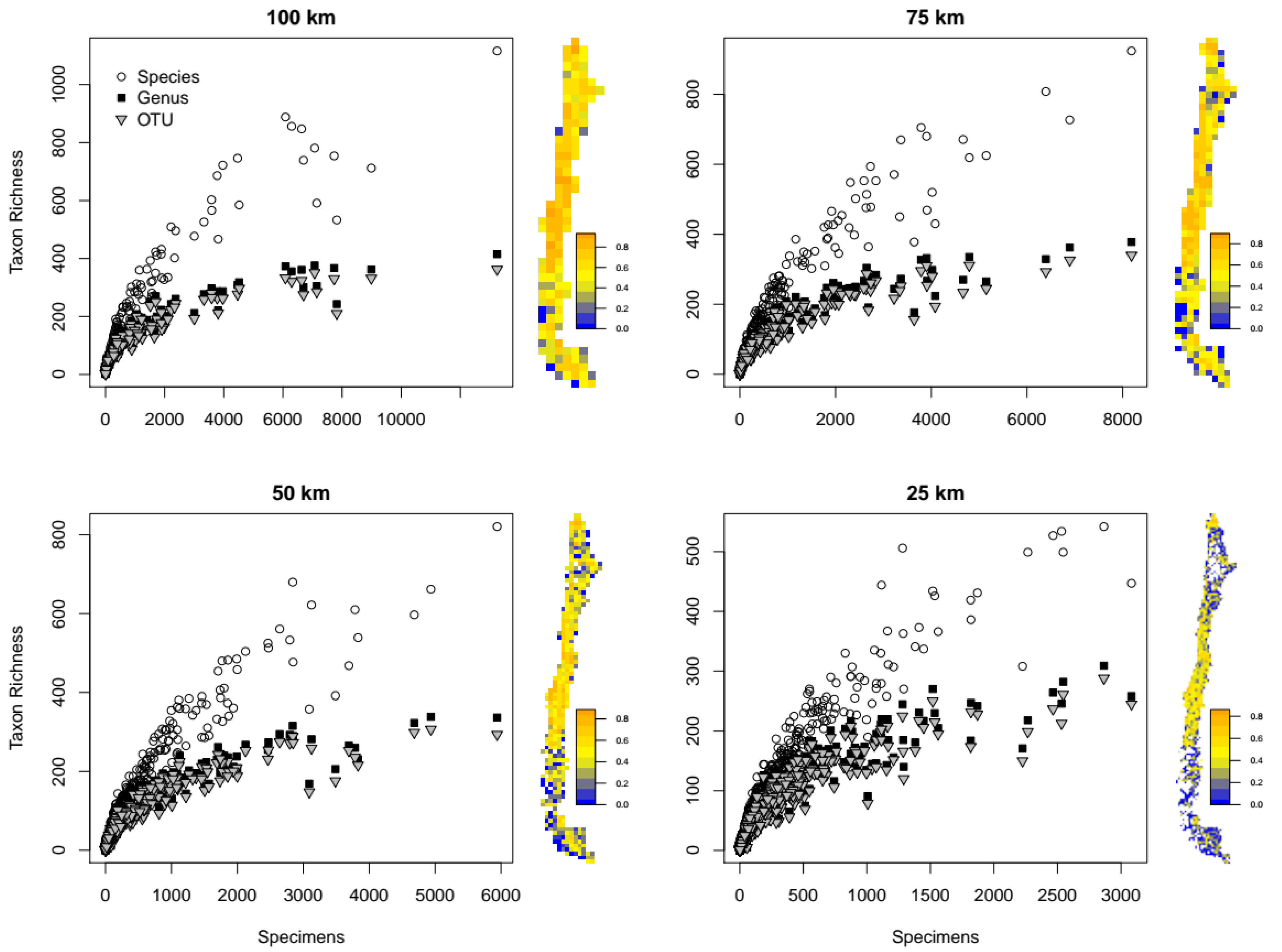
3.1. Redundancy and Grid Effects

Relationships between number of specimens and TR are depicted in Figure 1. Redundancy for the different spatial resolutions and taxonomic levels are presented in Figure 2. Average redundancy was greater than 0.6 for all taxonomic levels only at 100 km resolution and fell below this value for all taxonomic levels at 50 and 25 km resolution. At 75 km resolution, average redundancy was greater than 0.6 only for genera and OTUs.

Comparing average redundancy and average specimen-based fuzzy Kappa between the original and two shifted grids did not affect the results (Figure S1). We therefore present the results of the original grid.

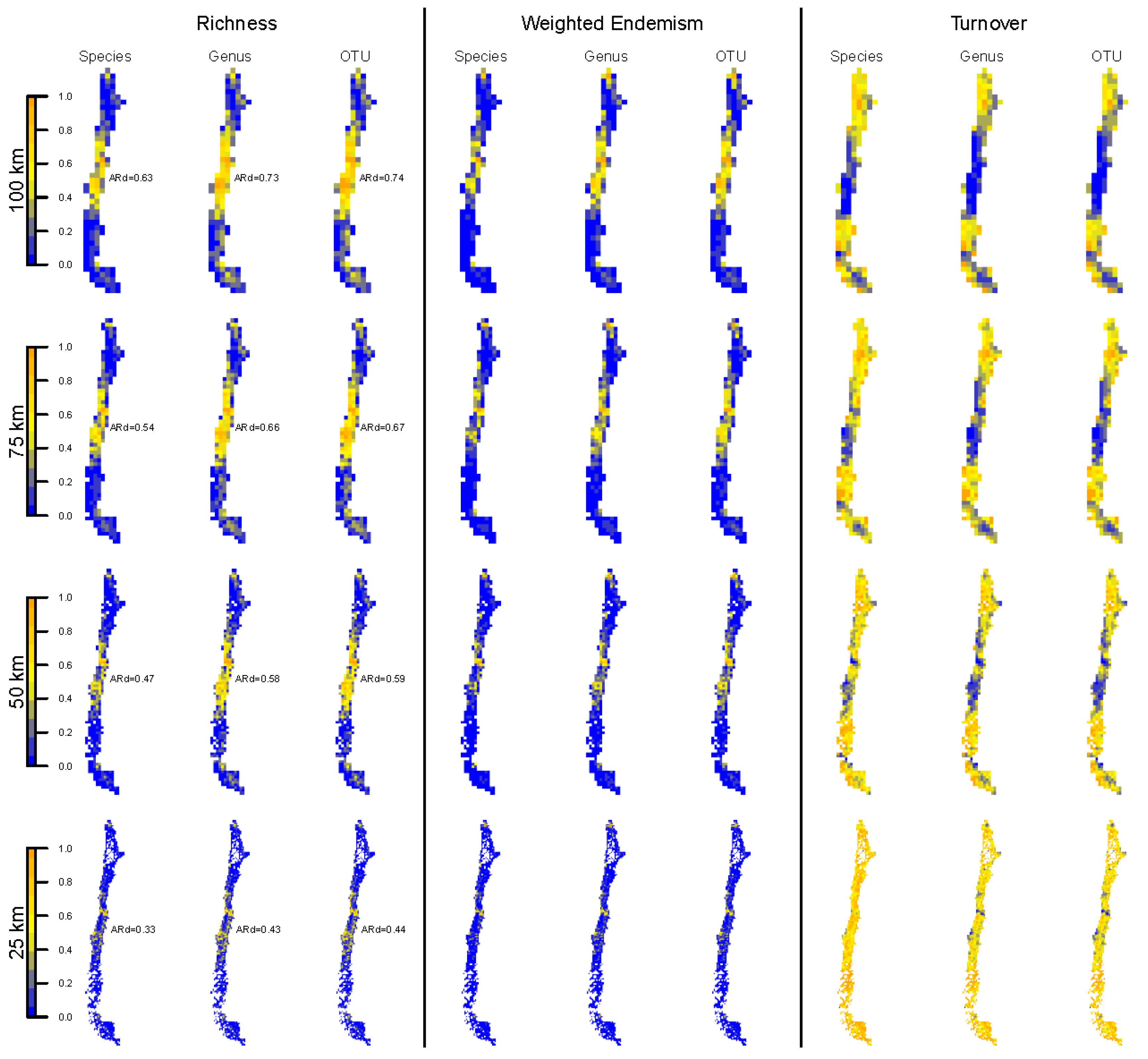
3.2. Spatial Patterns of Biodiversity—Specimen-Based Analyses

Spatial patterns of TR and WE (Figure 2, left and middle panels) were similar to each other within each spatial resolution (Figure S2). In both cases, the highest values were concentrated in the central part of Chile.

TT showed very similar spatial patterns among taxonomic levels within each spatial aggregation level (Figure 2, right panel, Figure S3). The largest TT values were concentrated in the northern and southern parts of Chile, while the central region showed lower values.

Agreement among taxonomic levels was higher and less variable between genera and OTUs than between species and genera and between species and OTUs at all resolutions and for all biodiversity indices, especially for WE (Figure 3A–C). Despite differences in spatial patterns among indices (Figure 2), average agreement tended to increase with spatial resolution, being the greatest at 25 km resolution for almost all comparisons between taxonomic scales and biodiversity indices (Figure 3A–C). Correlation between biodiversity indices for species vs. genera and OTUs was high at all resolutions (Figures S4–S6). Agreement in richness patterns between species and genera and between species and OTUs were inversely related to the ratio species/genera or species/OTUs (Figure S7).

Agreement between resolutions within taxonomic levels did not differ among taxonomic levels, but they did so between comparisons and biodiversity indices (Figure 3D–F). Fuzzy kappa values tended to be higher and less variable with respect to TT than both TR and WE. For all biodiversity indices, agreement was higher between similar resolutions (e.g., 100 vs. 75 km, 75 vs. 50 km) than between very different ones (e.g., 100 vs. 25 km, 75 vs. 25 km). The same pattern held for comparisons between both resolutions and taxonomic scales (Figure S8), though here the agreement values were lower and more variable.

3.3. Spatial Patterns—Mobile Windows

Mobile windows based on 25 km grid cells tended to show higher agreement between taxonomic scales than those based on 50 km grid cells both for TR and TT, but not for WE, which was low for comparisons between genus or OTU and species, regardless of resolution (Figure 4A–C). Comparison between mobile windows within taxonomic scales showed the same pattern for 50 km grid cells (Figure 4D–F) than for 25 km grid cells (Figure 4G–I), with better agreement for comparisons between larger windows for both TR and WE. For TT, agreement values were all higher than TR or WE except for larger mobile windows based on 25 km grid cells, which were slightly lower (Figure 4I).

Comparing between mobile windows and taxonomic levels (Figure S9) resulted in similar patterns for 50 and 25 km grid cell-based mobile windows. There was a trend towards higher agreement in TT (Figure S9C,F,I,L) than TR (Figure S9A,D,G,J) or WE (Figure S9B,E,H,K), no matter the resolution or direction. As in other analyses, poorest agreement was obtained for WE.

3.4. Spatial Patterns—SDM-Based Analyses

Using SDMs preserved the general distribution of all indices (Figure 5) with respect to the specimen-based analyses (compare Figure 2). TR and WE remained higher in the central part of the country and lower elsewhere (Figure 5, left and middle panels). Likewise, the pattern of TT tends to be the opposite (Figure 5, right panel), similar to the specimen-based analysis. This superficial similarity between specimen- and SDM-based analyses, however, does not translate into spatial agreement, which is generally low and decreases with increasing resolution (Figure 6A–C).

SDM agreement was higher between genera and OTUs than between these and species for all three indices (Figure 7A–C), but especially for WE (Figure 7B). However, average agreement between species vs. either OTUs or genera was higher in SDM-based analyses than in specimen-based analyses for TR and TT (compare Figure 3A,C and Figure 7A,C), a trend that remains unchanged across resolutions. The latter was not the case for WE, where a similar trend was observed in both specimen-based (Figure 3B) and SDM-based (Figure 7B) analyses.

Agreement between SDMs and specimen-based analyses between taxonomic scales tended to be similar to the results of the specimen-based analysis in TR (compare Figure 3A and Figure 6D), but not in WE and TT, where agreement was generally lower between SDM-based and specimen-based analyses (compare Figure 3B,C and Figure 6E,F), with genus–species and OTU–species agreement being lower than genus–OTU agreement in TR and WE (Figure 6D,E) but not in TT (Figure 6F).

3.5. Spatial Patterns of Species Richness—Mobile Windows of SDMs

Spatial agreement between taxonomic scales for SDMs was generally high regardless of resolution and mobile windows only for TR and TT (Figure 7D,F), but not for WE, where this was only true for genus–OTU agreement (Figure 7E). When mobile windows were compared between each other (Figures S10–S12), and the highest agreement was obtained between mobile windows with a radius ≥1, regardless of resolution (i.e., 50 or 25 km grid cell) and comparison (i.e., within and between taxonomic scales) only for TR, with exceptions for 50 km gird-cell (Figure S10A–C), and this was especially true for 25 km grid cell resolution (Figure S10D–F). SDMs tended to better surrogate specimen-based TR patterns at 25 km than 50 km grid cells, regardless of comparison (Figure S10G,H). The case of WE was different, with higher agreement for all comparisons within taxonomic scales (Figure S11A,D,G), and the least agreement for comparisons between species and either genus or OTU regardless of mobile window and resolution (Figure S11B,C,E,F,H,I). Howeverm a different trend was observed for TT, with generally high agreement between mobile windows irrespective of comparison (Figure S12A–F) and generally low agreement when SDM-based analyses were compared to specimen-based analyses, regardless of mobile window and resolution.

4. Discussion

Our analysis presents a comprehensive set of comparisons of three diversity indices for different spatial aggregation and taxonomic levels in order to understand how analyses at different taxonomic ranks and spatial resolutions may affect spatial patterns of diversity and how these spatial and taxonomic scales agree with each other both using specimen-based data and species distribution models (SDMs). The latter is a novel aspect of our study, the implication of which is that SDMs could be employed using higher taxa to create maps of higher taxon richness that would predict diversity indices, which would be useful in biodiverse countries with incomplete sampling. However, as discussed below, this might not always be the case.

We treated the spatial aggregation level in two ways. The first was employing an explicit measure of grain size by using four different square grid cells sizes (100, 75, 50 and 25 km grid cells). The second was by averaging diversity indices in mobile windows of three different radius for each of the two finest grids (50 and 25 km grid cells). The underlying purpose was supporting the use of surrogates of species-level data and lower spatial resolution to study biodiversity patterns. This study proposes a methodological approach to do it when data are scarce and biased. This issue is arguably even more relevant under the increasing interest of assessing biodiversity patterns using phylogenetic data (see below).

Literature has shown the scale-dependent nature of all indices tested here, namely taxon richness (e.g., [61]), endemism (e.g., [62]) and turnover (e.g., [63]). In light of that, our study sought to examine how different spatial scales can surrogate each other for different biodiversity indices within and among taxonomic levels. The default expectation is that, the more different the scales (both spatial and taxonomic), the less they should surrogate each other and, the higher the aggregation level the higher the surrogacy among taxonomic scales. The latter is expected because coarser resolutions tend to reduce the effects of incomplete sampling by aggregating the data into fewer spatial units. In most cases, this expectation holds, especially between spatial scales. Our discussion below is thus organized around the extent to which our findings conform to or depart from these expectations and what may be the methodological issues involved in such departures.

First, it is surprising that surrogacy seems to work better at finer scales, rather than broader scales. Laffan [60] suggests that higher aggregation levels can overestimate taxon distributions and hence explain why better agreements are obtained for finer resolutions. This trend is visible for all three biodiversity indices for specimen-based analyses (Figure 3A–C and Figure 4A–C), but not for SDM-based analyses (Figure 7A–C,J–L), suggesting that this apparent relationship might be an effect of sampling bias. The rationale behind this is the amplifying effect of low sampling effort on the species–area relationship [64,65], rendering high agreement due to many grid cells having only few taxa. Furthermore, these taxa are likely the most common ones, thus homogenizing the species pool across the landscape and affecting not only TR, but also WE and TT. High agreement values would then be concentrated around grid cells having low redundancy and low TR. This, on the other hand, highlights the correcting effects of SDMs. Besides, this result suggests that in areas with low sampling density, sampling bias may also misleadingly affect surrogacy values, skewing results towards higher agreement as resolution is refined.

Second, the extent to which taxonomic scales surrogate each other depends on which index is under analysis. Surrogacy is higher for TT than for TR and is the lowest for WE. The latter is expected, because the WE depends on the total area occupied by a taxon, and this is generally greater in genera and OTUs than in species. Comparing genera and species’ WE, might be seen as equivalent to a comparison between “splitters” and “lumpers” taxon views, which has recently been shown to have strong effects on spatial patterns of WE [66]. Low agreement between species and both genus and OTU remains low regardless of spatial aggregation level (Figure 3B and Figure 4B) or the use of SDMs (Figure 7B,K). Conversely, the use of SDMs tends to improve surrogacy for TR and TT (Figure 7A,C,J,L) compared to the specimen-based analyses (Figure 3A,C and Figure 4A,C).

Our analyses at different resolutions might be seen as essentially an exploration of the modifiable areal unit problem (MAUP). The most commonly discussed manifestation of this is in gerrymandering of political boundaries (e.g., [67]), but any aggregation of point events or samples from a continuous field to areal units is subject to this issue [68]. On the one hand, the coefficient of determination of a relationship tends to increase as the resolution is coarsened [69]. Our data do not show this trend (see, e.g., Figure S4). On the other hand, the coefficient of determination may vary depending on the arbitrarily chosen aggregation scheme [68]. In our case, this scheme is the square data structure of grid cells. We acknowledge the possibility of obtaining different outcomes under different aggregation schemes (e.g., using hexagon, rectangles or bricks’ data structures instead of squares; see [60]) and that this possibility was not explored. We are aware of no study dealing with biodiversity across scales investigating this.

Our study shows that using SDMs improve the quality of the results in terms of higher-rank taxon surrogacy for both TR and TT, but not for WE. The latter is to be expected since SDMs are applied only to those taxa with a minimum number of known unique occurrences, thus leaving out from the analysis those that are highly endemic. The fact that SDMs invariably increase the area of occupancy of the taxa, thus reducing endemism, should not affect surrogacy since this effect should occur at all taxonomic levels, though not to the same extent. For TR and TT, SDMs appear to contribute to alleviate the data density problem. Other approaches, such as using rarefaction curves, also appear to be capable to face this problem (e.g., [70]). However, rarefaction curves are not appropriate for TT because the identity of the species is lost. Laffan and Crisp [62] proposed a series of spatial randomizations of the data that may contribute to assess the uncertainty caused by incomplete sampling. The latter approach was not used in the present study, because, though appropriate for all TR, WE and TT, it does not provide new estimates of the indices, but rather gives information about their robustness in the face of the data density problem.

This paper shows how spatial patterns of biodiversity vary across taxonomic and spatial scales using Chile as an example. Even though Chile is a biodiversity hotspot [40], data availability is limited [45]. The latter is reflected in our redundancy analyses (Figure 1 and Figure 2), in which redundancy falls below a critical value at coarser spatial scales compared to other floristically better-known regions (e.g., California: [7]; Australia: [34]; Mediterranean Europe: [71]).

TR and WE are higher in central Chile at all taxonomic scales, confirming the results of previous studies [41]. This pattern appears to be the result of the combined effect of the global trend towards decreasing TR with latitude [72] and the fact the landscape in northern Chile is dominated by desert areas [73]. Conversely, turnover is lower in central Chile and tends to increase northwards and southwards at all spatial scales, which is shown in this study for the first time (Figure 2). There is a negative correlation between TR and TT. Since the measure used to calculate TT (Sørensen index) is independent of TR [74,75], this suggests that the vascular flora is spatially more homogeneous in central Chile than in the northern and southern regions in spite of its higher richness, at least at the spatial scales considered in this study. This is at odds with studies in other regions showing a general trend towards a positive relationship between alpha and beta diversity (e.g., [76]). However, this result should be viewed with caution because it may be influenced by the current gaps of floristic knowledge, considering that sampling effort tends to be higher in central Chile than in the northern and southern portions of the country (Figure 1). This trend towards a lower collecting effort in northern and southern Chile might lead to higher turnover due to species absence rather than species replacement [77]. Moreover, the absence of a taxon in a grid cell due to a low collecting effort represents a higher proportion of the taxon list in areas with low TR than in areas with high TR, causing TT to disproportionately rise in areas with low TR. The relationship between spatial patterns of alpha and beta diversity observed is likely a specific feature of our study area, but also depends on the metric chosen to measure alpha and beta diversity, and there are myriads of them with different properties (e.g., [50,51,74]). However, more general conclusions about the relationship between the spatial patterns of alpha and beta diversity remain to be derived, and this is undoubtedly a contribution to that discussion.

All three biodiversity indices (TR, WE and TT) at the species level are generally well-surrogated by the respective indices using genera and OTUs, i.e., they show high correlations (Figures S3–S5). However, there is spatial variation in the agreement when compared with the numerical Kappa index (Figure 3). Richness of higher taxa has been proposed to be an effective surrogate for species richness [78]. Species richness appears to be best predicted by richness of higher-rank taxa when the species to higher taxa ratio is low [79,80] and species richness is also low [81]. Thus, since most genera in the Chilean flora have only a few species (46% of genera are represented by one species and only 8% contain more than 15 species; [82]), a high level of agreement between species richness and higher-taxon richness is to be expected. The average agreement among taxonomic scales tends to increase with spatial resolution, but the spatial pattern varies depending on the biodiversity index. For TR and turnover, the highest agreement was found in the north and south of Chile, whereas for WE, the highest agreement was concentrated in the southern area of the country. For richness, the pattern of agreement is opposite to the pattern of richness itself, meaning that agreement is lower in central Chile, where TR is higher. This is to be expected if genera that inhabit the central area of the country have more species than those that inhabit the northern and southern regions, which was the tendency observed in our data (Figure S6). Conversely, for turnover, the pattern of agreement follows the pattern of turnover itself, i.e., agreement tends to be higher where TT is higher. The pattern of agreement in WE—higher in southern Chile—could be expected if the proportion of genera with restricted geographical ranges and few species is higher in southern Chile than elsewhere. While the latter seems to be the case (cf. Figure 3 and Figure S6; see Arroyo et al. [83]), the former would contradict Rapoport’s rule [84], which appears to hold in the Chilean flora [83].

Agreement in TR between species and genera or OTUs tends to be even higher when SDMs are incorporated. As SDMs are based on probability values, they tend to generate more continuous distribution patterns and correct collection bias, thus increasing the values of species richness in poorly sampled regions and underestimating them in species-rich areas [85,86,87,88,89]. Because of this, higher species–genus and species–OTU agreement in richness is to be expected if most of the higher-rank taxa are represented by only few species (see above).

Moreover, results of SDMs are strongly influenced by the spatial arrangement of the occurrence data [28]. This arrangement is biased by the accessibility and the relevance (botanical interests) of the sampled areas and tends to produce higher suitability in well-sampled places [90]. Therefore, the sampling problems in the estimation of diversity indices from specimen data are not completely overcome by using SDMs. Nonetheless, our results show that average agreement between specimen- and SDM-based TR is highest, and very similar, at 100 and 75 km resolution for all taxonomic scales. The similarity in the agreement of these two spatial resolutions favors using a 75 km grid cell size for this data set, since it is the highest possible resolution that still yields spatially congruent patterns. This may still be a too coarse a resolution for some conservation planning decisions that need to be made at a finer scale. While this might be seen as a limitation of our results and highlights the urgency for more occurrence data, some conservation strategies at a national level can benefit from these and other results on spatial patterns of biodiversity at this resolution.

Taken together, our results suggest that species diversity patterns in the Chilean vascular flora are best surrogated by higher-rank taxa at a 75 km spatial scale and making use of data derived from SDMs. The approach presented in this study can be applied to other areas to select an appropriate spatial scale and taxonomic level for downstream studies of PD. Even though generalizations in the specific spatial patterns presented here cannot be extrapolated to other areas, this approach can be applied to any area to select an appropriate spatial scale and taxonomic level for downstream biodiversity studies.

References

1. Ferrier, S. Mapping Spatial Pattern in Biodiversity for Regional Conservation Planning: Where to from Here? Syst. Biol. 2002, 51, 331–363. [Google Scholar] [CrossRef] [PubMed]
2. Foley, J.A.; DeFries, R.; Asner, G.P.; Barford, C.; Bonan, G.; Carpenter, S.R.; Chapin, F.S.; Coe, M.T.; Daily, G.C.; Gibbs, H.K.; et al. Global Consequences of Land Use. Science 2005, 309, 570–574. [Google Scholar] [CrossRef] [PubMed] [Green Version]
3. Thomas, C.D.; Cameron, A.; Green, R.E.; Bakkenes, M.; Beaumont, L.J.; Collingham, Y.C.; Erasmus, B.F.N.; de Siqueira, M.F.; Grainger, A.; Hannah, L.; et al. Extinction Risk from Climate Change. Nature 2004, 427, 145–148. [Google Scholar] [CrossRef]
4. Cardoso, P.; Erwin, T.L.; Borges, P.A.V.; New, T.R. The Seven Impediments in Invertebrate Conservation and How to Overcome Them. Biol. Cons. 2011, 144, 2647–2655. [Google Scholar] [CrossRef] [Green Version]
5. Mutke, J.; Weigend, M. Mesoscale Patterns of Plant Diversity in Andean South America Based on Combined Checklist and GBIF Data. Ber. R. Tüx. Ges. 2017, 29, 83–97. [Google Scholar]
6. Forest, F.; Grenyer, R.; Rouget, M.; Davies, T.J.; Cowling, R.M.; Faith, D.P.; Balmford, A.; Manning, J.C.; Procheş, Ş.; van der Bank, M.; et al. Preserving the Evolutionary Potential of Floras in Biodiversity Hotspots. Nature 2007, 445, 757–760. [Google Scholar] [CrossRef] [PubMed]
7. Baldwin, B.G.; Thornhill, A.H.; Freyman, W.A.; Ackerly, D.D.; Kling, M.M.; Morueta-Holme, N.; Mishler, B.D. Species Richness and Endemism in the Native Flora of California. Am. J. Bot. 2017, 104, 487–501. [Google Scholar] [CrossRef] [PubMed] [Green Version]
8. Ulloa Ulloa, C.; Acevedo-Rodríguez, P.; Beck, S.; Belgrano, M.J.; Bernal, R.; Berry, P.E.; Brako, L.; Celis, M.; Davidse, G.; Forzza, R.C.; et al. An Integrated Assessment of the Vascular Plant Species of the Americas. Science 2017, 358, 1614–1617. [Google Scholar] [CrossRef] [Green Version]
9. Erickson, D.L.; Jones, F.A.; Swenson, N.G.; Pei, N.; Bourg, N.A.; Chen, W.; Davies, S.J.; Ge, X.; Hao, Z.; Howe, R.W.; et al. Comparative Evolutionary Diversity and Phylogenetic Structure across Multiple Forest Dynamics Plots: A Mega-Phylogeny Approach. Front. Genet 2014, 5, 358. [Google Scholar] [CrossRef] [Green Version]
10. Zhang, H.-X.; Zhang, M.-L. Spatial Patterns of Species Diversity and Phylogenetic Structure of Plant Communities in the Tianshan Mountains, Arid Central Asia. Front. Plant Sci. 2017, 8, 2134. [Google Scholar] [CrossRef]
11. Gaston, K.J.; Williams, P.H. Mapping the World’s Species-The Higher Taxon Approach. Biodivers. Lett. 1993, 1, 2. [Google Scholar] [CrossRef]
12. Williams, P.H.; Gaston, K.J. Measuring More of Biodiversity: Can Higher-Taxon Richness Predict Wholesale Species Richness? Biol. Cons. 1994, 67, 211–217. [Google Scholar] [CrossRef]
13. Balmford, A.; Green, M.J.B.; Murray, M.G. Using Higher-Taxon Richness as a Surrogate for Species Richness: I. Regional Tests. Proc. Roy. Soc. B 1996, 263, 1267–1274. [Google Scholar] [CrossRef]
14. Viveiros Grelle, C.E. Is Higher-Taxon Analysis an Useful Surrogate of Species Richness in Studies of Neotropical Mammal Diversity? Biol. Cons. 2002, 108, 101–106. [Google Scholar] [CrossRef]
15. Cardoso, P.; Silva, I.; de Oliveira, N.G.; Serrano, A.R.M. Higher Taxa Surrogates of Spider (Araneae) Diversity and Their Efficiency in Conservation. Biol. Cons. 2004, 117, 453–459. [Google Scholar] [CrossRef]
16. Von Konrat, M.; Renner, M.; Söderström, L.; Hagborg, A.; Mutke, J. Early Land Plants Today: Liverwort Species Diversity and the Relationship with Higher Taxonomy and Higher Plants. Fieldiana. Bot. 2008, 2008, 91–104. [Google Scholar] [CrossRef]
17. Foord, S.H.; Dippenaar-Schoeman, A.S.; Stam, E.M. Surrogates of Spider Diversity, Leveraging the Conservation of a Poorly Known Group in the Savanna Biome of South Africa. Biol. Cons. 2013, 161, 203–212. [Google Scholar] [CrossRef]
18. Pérez-Fuertes, O.; García-Tejero, S.; Pérez Hidalgo, N.; Mateo-Tomás, P.; Cuesta-Segura, A.D.; Olea, P.P. Testing the Effectiveness of Surrogates for Assessing Biological Diversity of Arthropods in Cereal Agricultural Landscapes. Ecol. Indic. 2016, 67, 297–305. [Google Scholar] [CrossRef]
19. Pik, A.J.; Oliver, I.; Beattie, A.J. Taxonomic Sufficiency in Ecological Studies of Terrestrial Invertebrates. Aust. J. Ecol. 1999, 24, 555–562. [Google Scholar] [CrossRef]
20. Prinzing, A.; Klotz, S.; Stadler, J.; Brandl, R. Woody Plants in Kenya: Expanding the Higher-Taxon Approach. Biol. Cons. 2003, 110, 307–314. [Google Scholar] [CrossRef]
21. Mandelik, Y.; Dayan, T.; Chikatunov, V.; Kravchenko, V. Reliability of a Higher-Taxon Approach to Richness, Rarity, and Composition Assessments at the Local Scale. Cons. Biol. 2007, 21, 1506–1515. [Google Scholar] [CrossRef] [PubMed]
22. Groc, S.; Delabie, J.H.C.; Longino, J.T.; Orivel, J.; Majer, J.D.; Vasconcelos, H.L.; Dejean, A. A New Method Based on Taxonomic Sufficiency to Simplify Studies on Neotropical Ant Assemblages. Biol. Conserv. 2010, 143, 2832–2839. [Google Scholar] [CrossRef]
23. Andersen, A.N. Measuring More of Biodiversity: Genus Richness as a Surrogate for Species Richness in Australian Ant Faunas. Biol. Cons. 1995, 73, 39–43. [Google Scholar] [CrossRef]
24. Rosser, N.; Eggleton, P. Can Higher Taxa Be Used as a Surrogate for Species-Level Data in Biodiversity Surveys of Litter/Soil Insects? J. Insect. Conserv. 2012, 16, 87–92. [Google Scholar] [CrossRef]
25. Gaston, K.J. Biodiversity: Higher Taxon Richness. Prog. Phys. Geogr. 2000, 24, 117–127. [Google Scholar] [CrossRef] [Green Version]
26. Balmford, A.; Jayasuriya, A.H.M.; Green, M.J.B. Using Higher-Taxon Richness as a Surrogate for Species Richness: II. Local Applications. Proc. R. Soc. Lond. B 1996, 263, 1571–1575. [Google Scholar] [CrossRef]
27. Guisan, A.; Zimmermann, N.E. Predictive Habitat Distribution Models in Ecology. Ecol. Model. 2000, 135, 147–186. [Google Scholar] [CrossRef]
28. Guisan, A.; Thuiller, W.; Zimmermann, N.E. Habitat Suitability and Distribution Models: With Applications in R.; Cambridge University Press: Cambridge, UK, 2017; ISBN 978-0-521-75836-9. [Google Scholar]
29. Breiner, F.T.; Guisan, A.; Bergamini, A.; Nobis, M.P. Overcoming Limitations of Modelling Rare Species by Using Ensembles of Small Models. Meth. Ecol. Evol. 2015, 6, 1210–1218. [Google Scholar] [CrossRef]
30. Hernández, P.A.; Graham, C.H.; Master, L.L.; Albert, D.L. The Effect of Sample Size and Species Characteristics on Performance of Different Species Distribution Modeling Methods. Ecography 2006, 29, 773–785. [Google Scholar] [CrossRef]
31. Stockwell, D.R.B.; Peterson, A.T. Effects of Sample Size on Accuracy of Species Distribution Models. Ecol. Model. 2002, 148, 1–13. [Google Scholar] [CrossRef]
32. Scherson, R.A.; Thornhill, A.H.; Urbina-Casanova, R.; Freyman, W.A.; Pliscoff, P.A.; Mishler, B.D. Spatial Phylogenetics of the Vascular Flora of Chile. Mol. Phylogenet. Evol. 2017, 112, 88–95. [Google Scholar] [CrossRef] [PubMed]
33. Scherson, R.A.; Fuentes-Castillo, T.; Urbina-Casanova, R.; Pliscoff, P. Phylogeny-Based Measures of Biodiversity When Data Is Scarce: Examples with the Vascular Flora of Chile and California. In Phylogenetic Diversity: Applications and Challenges in Biodiversity Science; Scherson, R.A., Faith, D.P., Eds.; Springer International Publishing: Cham, Switzerland, 2018; pp. 131–144. ISBN 978-3-319-93145-6. [Google Scholar]
34. Thornhill, A.H.; Mishler, B.D.; Knerr, N.J.; González-Orozco, C.E.; Costion, C.M.; Crayn, D.M.; Laffan, S.W.; Miller, J.T. Continental-Scale Spatial Phylogenetics of Australian Angiosperms Provides Insights into Ecology, Evolution and Conservation. J. Biogeogr. 2016, 43, 2085–2098. [Google Scholar] [CrossRef]
35. Thornhill, A.H.; Baldwin, B.G.; Freyman, W.A.; Nosratinia, S.; Kling, M.M.; Morueta-Holme, N.; Madsen, T.P.; Ackerly, D.D.; Mishler, B.D. Spatial Phylogenetics of the Native California Flora. BMC Biol. 2017, 15, 96. [Google Scholar] [CrossRef] [PubMed] [Green Version]
36. Pio, D.V.; Broennimann, O.; Barraclough, T.G.; Reeves, G.; Rebelo, A.G.; Thuiller, W.; Guisan, A.; Salamin, N. Spatial Predictions of Phylogenetic Diversity in Conservation Decision Making. Cons. Biol. 2011, 25, 1229–1239. [Google Scholar] [CrossRef]
37. Pio, D.V.; Engler, R.; Linder, H.P.; Monadjem, A.; Cotterill, F.P.D.; Taylor, P.J.; Schoeman, M.C.; Price, B.W.; Villet, M.H.; Eick, G.; et al. Climate Change Effects on Animal and Plant Phylogenetic Diversity in Southern Africa. Glob. Chang. Biol. 2014, 20, 1538–1549. [Google Scholar] [CrossRef]
38. Mishler, B.D.; Knerr, N.; González-Orozco, C.E.; Thornhill, A.H.; Laffan, S.W.; Miller, J.T. Phylogenetic Measures of Biodiversity and Neo- and Paleo-Endemism in Australian Acacia. Nat. Commun. 2014, 5, 4473. [Google Scholar] [CrossRef]
39. Schmithüsen, J. Die Räumliche Ordnung Der Chilenischen Vegetation. Bonn. Geogr. Abh. 1956, 17, 1–86. [Google Scholar]
40. Myers, N.; Mittermeier, R.A.; Mittermeier, C.G.; da Fonseca, G.A.B.; Kent, J. Biodiversity Hotspots for Conservation Priorities. Nature 2000, 403, 853–858. [Google Scholar] [CrossRef]
41. Bannister, J.R.; Vidal, O.J.; Teneb, E.; Sandoval, V. Latitudinal Patterns and Regionalization of Plant Diversity along a 4270-km Gradient in Continental Chile. Aust. Ecol. 2012, 37, 500–509. [Google Scholar] [CrossRef]
42. Zuloaga, F.O.; Morrone, O.; Belgrano, M.J. Catálogo de Las Plantas Vasculares Del Cono Sur (Argentina, Sur de Brasil, Chile, Paraguay y Uruguay). Monogr. Syst. Bot. Mo. Bot. Gard. 2008, 107, 1–3348. [Google Scholar]
43. Echeverria, C.; Coomes, D.; Salas, J.; Rey-Benayas, J.M.; Lara, A.; Newton, A. Rapid Deforestation and Fragmentation of Chilean Temperate Forests. Biol. Cons. 2006, 130, 481–494. [Google Scholar] [CrossRef]
44. Urbina-Casanova, R.; Luebert, F.; Pliscoff, P.; Scherson, R.A. Assessing Floristic Representativeness in the Protected Areas National System of Chile: Are Vegetation Types a Good Surrogate for Plant Species? Environ. Cons. 2016, 43, 199–207. [Google Scholar] [CrossRef] [Green Version]
45. Simonetti, J.A. On the Size of the Chilean Flora (a Speculation). J. Medit. Ecol. 1999, 1, 129–132. [Google Scholar]
46. Garcillán, P.P.; Ezcurra, E.; Riemann, H. Distribution and Species Richness of Woody Dryland Legumes in Baja California, Mexico. J. Veg. Sci. 2003, 14, 475–486. [Google Scholar] [CrossRef]
47. R Core Team. R: A Language and Environment for Statistical Computing; R Foundation for Statistical Computing: Vienna, Austria, 2017. [Google Scholar]
48. Crisp, M.D.; Laffan, S.; Linder, H.P.; Monro, A. Endemism in the Australian Flora. J. Biogeogr. 2001, 28, 183–198. [Google Scholar] [CrossRef]
49. Laffan, S.W.; Rosauer, D.F.; Di Virgilio, G.; Miller, J.T.; González-Orozco, C.E.; Knerr, N.; Thornhill, A.H.; Mishler, B.D. Range-Weighted Metrics of Species and Phylogenetic Turnover Can Better Resolve Biogeographic Transition Zones. Meth. Ecol. Evol. 2016, 7, 580–588. [Google Scholar] [CrossRef]
50. Koleff, P.; Gaston, K.J.; Lennon, J.J. Measuring Beta Diversity for Presence-Absence Data. J. Anim. Ecol. 2003, 72, 367–382. [Google Scholar] [CrossRef] [Green Version]
51. Tuomisto, H. A Diversity of Beta Diversities: Straightening up a Concept Gone Awry. Part 1. Defining Beta Diversity as a Function of Alpha and Gamma Diversity. Ecography 2010, 33, 2–22. [Google Scholar] [CrossRef]
52. Guerin, G.R.; Ruokolainen, L.; Lowe, A.J. A Georeferenced Implementation of Weighted Endemism. Meth. Ecol. Evol. 2015, 6, 845–852. [Google Scholar] [CrossRef]
53. Oksanen, J.; Blanchet, F.G.; Friendly, M.; Kindt, R.; Legendre, P.; McGlinn, D.; Minchin, P.R.; O’Hara, R.B.; Simpson, G.L.; Solymos, P.; et al. Vegan: Community Ecology Package. 2018. Available online: http://cc.oulu.fi/~jarioksa/ (accessed on 27 September 2020).
54. Hijmans, R.J. Raster: Geographic Data Analysis and Modeling. R Package Version 2.8-19. Available online: https://CRAN.R-project.org/package=raster (accessed on 27 September 2020).
55. Phillips, S.J.; Anderson, R.P.; Schapire, R.E. Maximum Entropy Modeling of Species Geographic Distributions. Ecol. Model. 2006, 190, 231–259. [Google Scholar] [CrossRef] [Green Version]
56. Pliscoff, P.; Luebert, F.; Hilger, H.H.; Guisan, A. Effects of Alternative Sets of Climatic Predictors on Species Distribution Models and Associated Estimates of Extinction Risk: A Test with Plants in an Arid Environment. Ecol. Model. 2014, 288, 166–177. [Google Scholar] [CrossRef]
57. Di Cola, V.; Broennimann, O.; Petitpierre, B.; Breiner, F.T.; D’Amen, M.; Randin, C.; Engler, R.; Pottier, J.; Pio, D.; Dubuis, A.; et al. Ecospat: An R Package to Support Spatial Analyses and Modeling of Species Niches and Distributions. Ecography 2017, 40, 774–787. [Google Scholar] [CrossRef]
58. Pearson, R.G.; Raxworthy, C.J.; Nakamura, M.; Peterson, A.T. Predicting Species Distributions from Small Numbers of Occurrence Records: A Test Case Using Cryptic Geckos in Madagascar. J. Biogeogr. 2007, 34, 102–117. [Google Scholar] [CrossRef]
59. Visser, H.; de Nijs, T. The Map Comparison Kit. Environ. Model. Softw. 2006, 21, 346–358. [Google Scholar] [CrossRef]
60. Laffan, S.W. Phylogeny-Based Measurements at Global and Regional Scales. In Phylogenetic Diversity: Applications and Challenges in Biodiversity Science; Scherson, R.A., Faith, D.P., Eds.; Springer International Publishing: Cham, Switzerland, 2018; pp. 111–129. ISBN 978-3-319-93145-6. [Google Scholar]
61. Rahbek, C. The Role of Spatial Scale and the Perception of Large-Scale Species-Richness Patterns. Ecol. Lett. 2005, 8, 224–239. [Google Scholar] [CrossRef]
62. Laffan, S.W.; Crisp, M.D. Assessing Endemism at Multiple Spatial Scales, with an Example from the Australian Vascular Flora. J. Biogeogr. 2003, 30, 511–520. [Google Scholar] [CrossRef]
63. Barton, P.S.; Cunningham, S.A.; Manning, A.D.; Gibb, H.; Lindenmayer, D.B.; Didham, R.K. The Spatial Scaling of Beta Diversity. Glob. Ecol. Biogeogr. 2013, 22, 639–647. [Google Scholar] [CrossRef] [Green Version]
64. Adler, P.B.; White, E.P.; Lauenroth, W.K.; Kaufman, D.M.; Rassweiler, A.; Rusak, J.A. Evidence for a General Species–Time–Area Relationship. Ecology 2005, 86, 2032–2039. [Google Scholar] [CrossRef] [Green Version]
65. McGlinn, D.J.; Palmer, M.W. Modeling the Sampling Effect in the Species–Time–Area Relationship. Ecology 2009, 90, 836–846. [Google Scholar] [CrossRef] [Green Version]
66. Daru, B.H.; Farooq, H.; Antonelli, A.; Faurby, S. Endemism Patterns Are Scale Dependent. Nat. Commun. 2020, 11, 2115. [Google Scholar] [CrossRef]
67. Nelson, J.K.; Brewer, C.A. Evaluating Data Stability in Aggregation Structures across Spatial Scales: Revisiting the Modifiable Areal Unit Problem. Cartogr. Geogr. Inf. Sci. 2017, 44, 35–50. [Google Scholar] [CrossRef]
68. Openshaw, S. The Modifiable Areal Unit Problem. Concepts Tech. Modern Cartogr. 1983, 38, 1–41. [Google Scholar]
69. O’Sullivan, D.; Unwin, D.J. Geographic Information Analysis, 2nd ed.; John Wiley & Sons: Hoboken, NJ, USA, 2010; ISBN 978-0-471-21176-1. [Google Scholar]
70. Alroy, J. Limits to Species Richness in Terrestrial Communities. Ecol. Lett. 2018, 21, 1781–1789. [Google Scholar] [CrossRef] [PubMed]
71. Medail, F.; Quezel, P. Hot-Spots Analysis for Conservation of Plant Biodiversity in the Mediterranean Basin. Ann. Mo. Bot. Gard. 1997, 84, 112–127. [Google Scholar] [CrossRef]
72. Gaston, K.J.; Spicer, J.I. Biodiversity: An Introduction, 2nd ed.; Blackwell Science: Oxford, UK, 2004; ISBN 978-1-4051-1857-6. [Google Scholar]
73. Luebert, F.; Pliscoff, P. Sinopsis Bioclimática y Vegetacional de Chile, 2nd ed.; Editorial Universitaria: Santiago, Chile, 2017. [Google Scholar]
74. Jost, L. Partitioning Diversity into Independent Alpha and Beta Components. Ecology 2007, 88, 2427–2439. [Google Scholar] [CrossRef] [Green Version]
75. Tuomisto, H. A Diversity of Beta Diversities: Straightening up a Concept Gone Awry. Part 2. Quantifying Beta Diversity and Related Phenomena. Ecography 2010, 33, 23–45. [Google Scholar] [CrossRef]
76. Qian, H.; Ricklefs, R.E. A Latitudinal Gradient in Large-Scale Beta Diversity for Vascular Plants in North America. Ecol. Lett. 2007, 10, 737–744. [Google Scholar] [CrossRef]
77. Harrison, S.; Ross, S.J.; Lawton, J.H. Beta Diversity on Geographic Gradients in Britain. J. Anim. Ecol. 1992, 61, 151–158. [Google Scholar] [CrossRef]
78. Gaston, K.J.; Blackburn, T.M. Mapping Biodiversity Using Surrogates for Species Richness: Macro-Scales and New World Birds. Proc. R. Soc. Lond. B 1995, 262, 335–341. [Google Scholar] [CrossRef]
79. La Ferla, B.; Taplin, J.; Ockwell, D.; Lovett, J.C. Continental Scale Patterns of Biodiversity: Can Higher Taxa Accurately Predict African Plant Distributions? Bot. J. Linn. Soc. 2002, 138, 225–235. [Google Scholar] [CrossRef]
80. Rosser, N. Shortcuts in Biodiversity Research: What Determines the Performance of Higher Taxa as Surrogates for Species? Ecol. Evol. 2017, 7, 2595–2603. [Google Scholar] [CrossRef]
81. Neeson, T.M.; Rijn, I.V.; Mandelik, Y. How Taxonomic Diversity, Community Structure, and Sample Size Determine the Reliability of Higher Taxon Surrogates. Ecol. Appl. 2013, 23, 1216–1225. [Google Scholar] [CrossRef] [PubMed] [Green Version]
82. Moreira-Muñoz, A. Plant Geography of Chile; Springer: Dordrecht, The Netherlands, 2011. [Google Scholar]
83. Arroyo, M.T.K.; Riveros, M.; Peñaloza, A.; Cavieres, L.A.; Faggi, A.M. Phytogeographic Relationships and Regional Richness Patterns of the Cool Temperate Rainforest Flora of Southern South America. In High-Latitude Rainforest and Associated Ecosystems of the West Coast of the Americas; Lawford, R.G., Alaback, P., Fuentes, E., Eds.; Springer: New York, NY, USA, 1996; pp. 134–172. [Google Scholar]
84. Stevens, G.C. The Latitudinal Gradient in Geographical Range: How so Many Species Coexist in the Tropics. Am. Nat. 1989, 133, 240–256. [Google Scholar] [CrossRef]
85. Pineda, E.; Lobo, J.M. Assessing the Accuracy of Species Distribution Models to Predict Amphibian Species Richness Patterns. J. Anim. Ecol. 2009, 78, 182–190. [Google Scholar] [CrossRef]
86. Raes, N.; Roos, M.C.; Slik, J.W.F.; Loon, E.E.V.; Steege, H.t. Botanical Richness and Endemicity Patterns of Borneo Derived from Species Distribution Models. Ecography 2009, 32, 180–192. [Google Scholar] [CrossRef] [Green Version]
87. Calabrese, J.M.; Certain, G.; Kraan, C.; Dormann, C.F. Stacking Species Distribution Models and Adjusting Bias by Linking Them to Macroecological Models. Glob. Ecol. Biogeogr. 2014, 23, 99–112. [Google Scholar] [CrossRef]
88. Pouteau, R.; Bayle, É.; Blanchard, É.; Birnbaum, P.; Cassan, J.-J.; Hequet, V.; Ibanez, T.; Vandrot, H. Accounting for the Indirect Area Effect in Stacked Species Distribution Models to Map Species Richness in a Montane Biodiversity Hotspot. Divers. Distrib. 2015, 21, 1329–1338. [Google Scholar] [CrossRef]
89. Zhang, M.-G.; Slik, J.W.F.; Ma, K.-P. Using Species Distribution Modeling to Delineate the Botanical Richness Patterns and Phytogeographical Regions of China. Sci. Rep. 2016, 6, 22400. [Google Scholar] [CrossRef] [Green Version]
90. Kadmon, R.; Farber, O.; Danin, A. Effect of Roadside Bias on the Accuracy of Predictive Maps Produced by Bioclimatic Models. Ecol. Appl. 2004, 14, 401–413. [Google Scholar] [CrossRef]
Figure 1. Taxon richness plotted as a function of number of specimens at different taxonomic levels (species, genus and OTU) and spatial resolutions (100, 75, 50 and 25 km grid cells). Maps next to the charts show the spatial distribution of species redundancy for the corresponding resolution.
Diversity 14 00271 g001
Figure 2. Spatial distribution of specimen-based biodiversity indices (taxon richness, weighted endemism and turnover) at different taxonomic levels (species, genus and OTU) and spatial resolutions (100, 75, 50 and 25 km grid cells). All biodiversity indices were transformed to percentages to obtain a comparable, common scale across indices. The average redundancy (“ARd”) for the corresponding taxonomic level and spatial resolution is shown next to each map of the left panel. The spatial distribution depicted maps the geographic boundaries of Chile.
Diversity 14 00271 g002
Figure 3. Average spatial agreement measured with the fuzzy Kappa index for taxon richness, weighted endemism and taxon turnover, based on specimen data. (AC): comparisons between taxonomic levels (species, genus and OTU) at different spatial resolutions (100, 75, 50 and 25 km grid cells). (DF): comparisons within taxonomic levels and between spatial resolutions.
Diversity 14 00271 g003
Figure 4. Average spatial agreement measured with the fuzzy Kappa index for taxon richness (left panel), weighted endemism (middle panel) and turnover (right panel), based on specimen data for different mobile windows. (AC): comparisons between taxonomic levels (species, genus and OTU) at different spatial resolutions (50 and 25 km grid cells) and mobile windows (MW1, MW2 and MW3). (DF): comparisons within taxonomic levels between mobile windows for 50 km grid cells. (GI): same as (DF) but for 25 km grid cells.
Diversity 14 00271 g004
Figure 5. Spatial distribution of SDM-based biodiversity indices (taxon richness, weighted endemism and turnover) at different taxonomic levels (species, genus and OTU) and spatial resolutions (100, 75, 50 and 25 km grid cells). All biodiversity indices were transformed to percentages to obtain a comparable, common scale across indices. The spatial distribution depicted maps the geographic boundaries of Chile.
Diversity 14 00271 g005
Figure 6. Average spatial agreement measured with the fuzzy Kappa index for taxon richness (A,D), weighted endemism (B,E) and turnover (C,F) between specimen-based and SDM-based analyses. (AC): comparison within taxonomic levels, for different spatial resolutions. (DF): Comparison between taxonomic scales for different spatial resolutions.
Diversity 14 00271 g006
Figure 7. Average spatial agreement measured with the fuzzy Kappa index for taxon richness (A,D), weighted endemism (B,E) and turnover (C,F) using species distribution models (SDMs). (AC): Comparison between taxonomic levels (species, genus and OTU) for different spatial resolutions (100, 75, 50 and 25 km grid cells). (DF): Comparison between taxonomic scales for different spatial resolutions (50 and 25 km grid cells) and mobile windows (MW1, MW2 and MW3).
Diversity 14 00271 g007
Publisher’s Note: MDPI stays neutral with regard to jurisdictional claims in published maps and institutional affiliations.