Abstract
β-diversity has been under continuous debate, with a current need to better understand the way in which a new wave of measures work. We assessed the results of 12 incidence-based β-diversity indices. Our results of gradual species composition overlap between paired assemblages considering progressive differences in species richness show the following: (i) four indices (β-2, β-3, β-3.s, and βr) should be used cautiously given that results with no shared species retrieve results that could be misinterpreted; (ii) all measures conceived specifically as partitioned components of species compositional dissimilarities ought to be used as such and not as independent measures per se; (iii) the non-linear response of some indices to gradual species composition overlap should be interpreted carefully, and further analysis using their results as dependent variables should be performed cautiously; and (iv) two metrics (βsim and βsor) behave predictably and linearly to gradual species composition overlap. We encourage ecologists using measures of β-diversity to fully understand their mathematical nature and type of results under the scenario to be used in order to avoid inappropriate and misleading inferences.
1. Introduction
Since its birth with Whittaker’s proposal in 1960 (considering previous work–e.g., Jaccard [1]; Koch [2]), β-diversity, taken in its broadest sense as the relative change in species composition between two or more communities in space and/or time, has been under continuous debate in the ecological literature, both theoretically and practically. Undoubtedly, previous studies dealing with β-diversity have contributed immensely to our current understanding of the variability in species composition among sampling units. However, differences in the way we conceive and calculate β-diversity have resulted in multiple interpretations of the compositional dissimilarity of ecological communities (e.g., differentiation, species turnover, scaling, variance [3,4,5,6]). This differential interpretation of β-diversity has resulted in the proposal of a diverse array of measures, mostly focused on the refinement of their mathematical basis (e.g., Wilson and Shmida [7]), and often overseeing their ecological interpretation [8]. Notably, Whittaker further defined β-diversity as a quotient of diversities (i.e., γ/α), establishing the basis for its consideration as proportional diversity [9,10,11]. This particular topic is not addressed in this paper.
In 2003, Koleff et al. [12] assessed and synthesized the performance of the large array of β-diversity measures available at that time. Specifically, the authors undertook a comparative analysis of 24 β-diversity measures focusing on four mathematical properties: symmetry (for two quadrats x and y, β (x,y) must be equal to β (y,x)), homogeneity (if the components of the measure are multiplied by the same constant, this should not affect the resulting β-diversity value), nestedness (all the species occurring in the focal quadrat also occur in the neighboring quadrat), and additivity (for three quadrats in the spatial sequence x, y, z, the sum of the values of beta diversity between x and y and between y and z equals the value of beta diversity between x and z). After carrying out a thorough and robust set of analyses, they concluded that none of the evaluated measures accomplished all of the assessed mathematical properties, and only nine of them reflected the gain and loss of species. Only four of all assessed indices performed well for three of the four tested criteria: βr, β-2, β-3, and βsim. Finally, Koleff et al. [12] highlighted the behavior of βsim given its acceptable performance under the additivity property. Yet, β-2 and β-3 (the modified version of this latter) have been found robust to undersampling, understood as another desirable property of these types of indices [13].
Recently, several studies have revisited the nestedness property of β-diversity, which describes the sub-setting of the species of species-poor sites in relation to species-rich ones (e.g., Baselga [14,15]; Carvalho et al. [16]; Baselga and Leprieur [17]). Specifically, the additive partitioning of β-diversity—initially proposed by Baselga [14]—identifies and differentiates the two separate resultant components (i.e., nestedness and turnover, with the latter representing the number of species that are replaced between sites in relation to the total number of species that could be replaced, also called “species replacement” [15]) underlying the total amount of β-diversity. As such, this additive partitioning of β-diversity is not related with other proposed additive partitioning of diversity that follow a different rationale (i.e., β-diversity = γ/α) [10,18]. Nonetheless, a wave of publications has populated the literature focusing on the development and application of the partitioning of β-diversity. Although there are elements of the proposed partitioning approach that have been criticized (e.g., inconsistency with the variation of species replacement and species loss, failure to accurately represent the species replacement and species loss processes, independence of richness difference; lack of connections to any other nestedness indices, overrepresentation of the replacement component due to the scaling difference; Almeida-Neto et al. [19]; Chen and Schmera [20]; Podani and Schmera [21,22]), it has recently gained relevance in the literature due to the information that it can provide on different ecological processes related to changes in species composition among communities, with topics ranging from genetic to biogeographical diversity (e.g., Diniz-Filho et al. [23]; Mouillot et al. [24]; Norhazrina et al. [25]; Ramachandran et al. [26]).
It is crucial to highlight that, by definition, partitioned indices should be considered in light of their related dissimilarity index given their interdependence with it [14,15,16,17,27,28]. As clearly stated by Murray and Baselga [29], measures proposed to partition β-diversity (i.e., nestedness/richness differences, replacement) are not independent measures, but quantifications of how dissimilar two assemblages are because of nestedness, replacement, and/or richness differences (although previous studies have considered βsim as an independent turnover index [30]). In addition to previous criticisms to the partitioning approach [19,20], we have identified studies using some of the newly suggested β-diversity measures as independent descriptors in further statistical analyses. To name a few examples, Georgopoulou et al. [31] used βjtu as an independent dissimilarity measure to represent the turnover component of Jaccard dissimilarity (sensu Baselga and Leprieur [17]). Although they recognize that partition identity of βsne and βsim, Koyanagi et al. [32] use both indices as independent measures and as dependent variables for further analyses (i.e., PCoA, GLM). Regarding the interpretation of the indices results and partitions, studies have not only used indices such as βj, βsim, and βsne in subsequent statistical analyses, but have even transformed them (i.e., arcsin transformation) based on the assumption that they range from 0–1, when two of the considered indices are used as partitions [33]. Therefore, caution is needed when comparing and interpreting the results of these studies that have not used β-diversity measures as they are intended, as they could be spurious and/or uninformative.
The main goal of this study was to evaluate the performance of 12 incidence-based β-diversity indices under different scenarios (see Table 1 for their mathematical formula and interpretation): two classical and widely used measures (i.e., βj, βsor), four measures that have been demonstrated to be symmetric, homogeneous, and sensitive to nestedness by Koleff et al. [12] (i.e., βsim, βr, β-2, β-3), and six recently proposed measures related to the partitioning of β-diversity (i.e., βsne, βrich, βjne, βjtu, βrich.s, β-3.s; reviewed in Baselga and Leprieur [17]). Notably, here we do not attempt to test the applicability or robustness of each β-diversity index (including their partitioning components), nor do we attempt to contrast results to a standard. Instead, our intention is to clearly show how the results of these measures behave based on previously hypothetical scenarios of assemblages used in Baselga [14], as well as new scenarios. This approach allowed us to group indices based on the nature of their results. We also tested the role of species richness differences in molding the type of results the 12 studied measures produced by controlling for the number of shared species. Finally, we studied scenarios of gradual species composition overlap between paired assemblages considering progressive differences in species richness.

Table 1.
List of assessed incidence-based β-diversity measures. Formulas were retrieved from the R packages ‘betapart’ (Baselga et al. [34]) and function ‘betadiver’ of the ‘vegan’ package (Oksanen et al. [35]). ‘a’: total number of species that occur in both assemblages (shared species); ‘b’ and ‘c’: number of species that occur in one assemblage but not in the other (exclusive species).
2. Materials and Methods
In order to assess the type of results of the 12 assessed measures (Table 1), we used two sets of scenarios (Figure 1). First, we retrieved the four hypothetical scenarios used in Baselga [14] (p. 135, examples A–D) that aim to account for (i) nestedness, (ii) spatial turnover, (iii) nestedness and spatial turnover, as well as (iv) differences in richness (referred to as Baselga’s Scenarios hereafter). Second, given that Baselga’s Scenarios seem simplistic, we generated a set of scenarios differing in species richness that contrast a reference hypothetical assemblage with assemblages sharing all species, sharing half of the species, and sharing no species as follows: 1:1 (i.e., 6 vs. 6 sp.), 1:0.5 (i.e., 12 vs. 6 sp., and 1:0.16 ratios (i.e., 25 vs. 4 sp.) (referred to as new scenarios hereafter; Figure 1). We used this set of new scenarios in order to test if the role of species richness differences controlling for the number of shared species changed in relation to Baselga’s Scenarios. We are specifically considering highly contrasting assemblage arrangements that resemble those commonly found in conditions of the Anthropocene (e.g., grazing pastures, croplands, urban settings [36]).
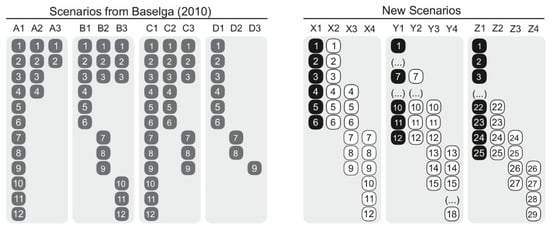
Figure 1.
Hypothetical scenarios used in this study: Baselga’s Scenarios (left), retrieved from Baselga [14], that aim to account for nestedness (sites A), spatial turnover (sites B), turnover and nestedness (sites C), and turnover and differences in species richness (sites D); new scenarios (right), with a set of hypothetical assemblages differing in species richness contrasting a reference hypothetical assemblage (black) with assemblages sharing all species, sharing half of the species, and sharing no species (white).
We generated pairwise calculations for Baselga’s Scenarios and the new scenarios using the functions ‘betadiver’ and ‘betapart’ [34] of the package ‘vegan’ [35] for R [37]. Given that, to our knowledge, no function or R package calculates βrich, βrich.s, β-3.s, we included the formulas of these measures in ‘betadiver’ as expressed in Baselga and Leprieur [17] (see Table 1 for details). In order to assess the similarities/dissimilarities of the results of the assessed measures, we performed a two-dimension non-metric multidimensional scaling (NMDS) analysis using Euclidean distances. For consistency, we re-expressed all results for these analyses to dissimilarity and present them in the Supplementary Material. We followed an NMDS approach as it represents one of the most robust unconstrained ordination methods in ecology to graphically represent the similarities among the assessed measures in a two-dimensional plot, often summarizing more information in a lower number of axes and lacking limitations regarding sample size, scale, and normality [38]. In order to validate our interpretation of the NMDS grouping, we ran an analysis to fit the interpreted groupings (a vector) to the ordination using the ‘envfit’ function for the package ‘vegan’ (beta calculations can also be run on BAT [39]).
We then assessed the results of the 12 measures through gradual species composition overlap between paired assemblages, considering progressive differences in species richness (Figure 2). This approach allowed us to record the results of the 12 focal indices in differing species richness and overlap scenarios. Briefly, we contrasted 10 hypothetical assemblages (Assemblage Bn) ranging from 1–10 species with a 10 species reference assemblage (Assemblage A). To evaluate differences in gradual species composition overlap, we performed pairwise calculations between Assemblage A and Assemblages B1–10, retrieving the results for all possible combinations ranging from sharing all species to sharing none (see Figure 2 for a graphical example of 10 vs. 5 species). This procedure would not only show how the studied indices behave when gradually changing from entirely nested to entirely turned over, but also assess the importance of differences in species richness between the gradually overlapped paired assemblages on β-diversity measures and results.
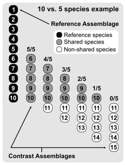
Figure 2.
Example of a gradual species composition overlap between two paired assemblages considering progressive differences in species richness. The hypothetical reference assemblage has 10 species and the contrast assemblage has five species. To evaluate differences in gradual species composition overlap, we performed pairwise calculations between the reference assemblage and those sharing 5–0 species with it.
We further tested potential relationships between the total species richness of randomly generated paired assemblages and the results of the 12 assessed indices. For this, we generated 100 paired random assemblages ranging from 11 to 1000 species with three different richness ratios: 1:1, 1:0.5, and 1:0.1. We then retrieved the results of the 12 assessed indices for all randomly generated paired assemblages. Finally, in order to assess potential relationships between matrix size and the type of results and the studied indices, we calculated Spearman correlations for the results of all assessed indices and the total species richness of randomly generated paired assemblages (matrix size; Figure S1) considering highly conservative Holm–Bonferroni sequential adjustments of p-values [40].
It is of the utmost importance to clarify that, given the goal of this study, which is to assess the type of results of the 12 measures calculated using the trending environment for statistical computing R [37], we kept the original formulas (some of similarity, others of dissimilarity) and thus did not re-express formulas to homogenize results (as performed in some previous studies; e.g., Koleff et al. [12]; Baselga and Leprieur, [17]; Table 1) for our gradual species composition overlap (yet, we do include the homogenized results in Figure S2). The latter ensures that the interpretation of the results is not misguided in relation to the original description of the measures. Nonetheless, we have included results with re-expressed formulas in the Supplementary Material in order to allow comparisons with previous studies.
3. Results
Through NMDS ordinations, we found that the retrieved similarity/dissimilarity values of all calculations were highly similar between both sets of hypothetical scenarios, showing that Baselga’s Scenarios are robust for index assessment (Table S1, Figure 3). Both NMDSs were highly fit (Baselga’s scenarios: stress = 0.03, linear fit r2 = 0.99; new scenarios: stress = 0.01, linear fit r2 = 0.99), indicating that they are reliable. Interestingly, results of both NMDSs show that there are some measures whose results are highly similar, grouping them together in the two-dimensional space (with the new scenarios increasing their similarity). Specifically, we detected five groups: (i) both classic measures (i.e., βj, βsor), (ii) both nestedness measures (i.e., βsne, βjne), (iii) both measures that take into account species richness difference (i.e., βrich, βrich.s), (iv) both turnover measures (i.e., βsim, βjtu), and (v) the four remaining dissimilarity and replacement measures (i.e., βr, β-2, β-3, β-3.s). These groups were significantly correlated with the ordination of index results (Baselga’s Scenarios: r2 = 0.97, p = 0.001, new scenarios r2 = 0.97, p < 0.001).
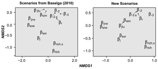
Figure 3.
Non-metric multidimensional scaling (NMDS) analyses showing the similarities/dissimilarities of the results of the 12 assessed measures with both sets of scenarios (see Figure S1). Arrows indicate the true location of indices, which were moved for graphical purposes.
Regarding the gradual species composition overlap analysis between paired assemblages considering progressive differences in species richness, the results of the assessed measures were highly variable (Figure 4). Here, we focus on the results of each measure by contrasting the groups shown by the NMDSs, some of which were expected, and some of which were not (i.e., group 5). For group 1, βj and βsor showed a positive increase in similarity with the proportion of assemblage overlap, which was heavily influenced by differences in species richness. It is noteworthy that βsor increased linearly and βj non-linearly (see Figure S2 for results with re-expressed formulas to show dissimilarity patterns). For group 2, we found a positive increase in both measures (i.e., βsne, βjne) with the proportion of assemblage overlap, which was linear for βsne and non-linear for βjne (Figure 4); both measures were also found to be highly influenced by species richness differences. Notably, none of the results of both measures reached 1, as expected due to the nature of the partition measure; maximum values were 0.82 for βsne and 0.9 for βjne, even in scenarios of 100% nestedness.
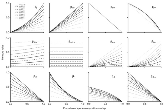
Figure 4.
Gradual species composition overlap between paired assemblages considering progressive differences in species richness.
Both measures of group 3 (i.e., βrich, βrich.s) were very sensitive to changes in species richness; βrich.s behaved linearly and βrich tended to be non-linear. It is important to highlight that, on the one hand, βrich was mildly influenced by the proportion of overlap, with increasingly higher values between absent and total overlap (i.e., 10 vs. 9 sp. = 5%, 10 vs. 8 sp. = 9%, 10 vs. 7 sp. = 12%, 10 vs. 6 sp. = 15%, 10 vs. 5 and 4 sp. = 17%, 10 vs. 3 sp. = 16%, 10 vs. 2 sp. = 13%, 10 vs. 1 sp. = 8%). On the other hand, the results of βrich.s were not equidistant with differences in species richness, with larger intervals among higher values and smaller intervals among lower values (e.g., Δ βrich.s 1–2 sp. = 0.15; Δ βrich.s 9–10 sp. = 0.05).
Regarding turnover measures of group 4 (i.e., βsim, βjtu), both decreased with the proportion of assemblage overlap, with βsim showing a linear pattern regardless of differences in species richness and βjtu behaving non-linearly when the poorest assemblage has more than two species (given that the comparison with the assemblage of one species only generates two results that result in a linear response). For group 5 (i.e., βr, β-2, β-3, β-3.s), indices showed different patterns, but one general similarity: all retrieved unexpected values (>1) with no shared species when the species richness of the contrast assemblage was = 1–9. Moreover, β-3 behaved non-linearly with maximum values = 0.5, and β-r also showed non-linear results. β-2 and β-3.s decreased linearly with proportion of assemblage overlap; the former returned equidistant decreasing values with larger differences in species richness, and the latter returned lesser differences with lesser species richness differences (Figure 4).
Finally, according to the assessment of index susceptibility to the matrix size (given by the total species richness of randomly generated paired assemblages), we found non-significant relationships with a 1:1 species richness ratio. We only recorded one moderate and significant relationship for βrich.s with a 1:0.5 ratio, as well as two significant, moderate and weak, positive relationships for βrich and βrich.s, respectively (Table S2; Figure S1).
4. Discussion
More than half a century after Whittaker [41] formally coined the definition of β-diversity, and over a century after Jaccard’s [1] pioneering ‘coefficient of community’ approach, we still lack a consensus on the ways to quantify it in any of its expressions (see Moreno and Rodríguez [3]), as well as in the criteria for their use and ecological interpretation. Our results show that all assessed measures were not susceptible to matrix size (except βrich and βrich.s in scenarios with differing species richness, as would be expected due to their mathematical nature). Moreover, we show several performance aspects of the 12 assessed β-diversity measures worth taking into account when choosing indices, as well as when using and interpreting them. Results for the NMDSs were highly similar between the sets of hypothetical scenarios, both of which showed how the 12 assessed indices group in five clusters (classic measures: βj, βsor; nestedness measures: βsne, βjne; species richness difference methods: βrich, βrich.s; turnover measures: βsim, βjtu; remaining dissimilarity/replacement measures: βr, β-2, β-3, β-3.s). These findings indicate that, although differences exist, classic, nestedness, species richness difference, and turnover metrics retrieve results in a similar fashion.
In this section, we first focus on the measures that, having a ‘dissimilarity’ nature, returned values differing from 1, often when species richness was not equal between samples and in non-overlap scenarios (i.e., no shared species). Second, we address the implications of the non-linear responses of some of the assessed β-diversity measures to the gradual species composition overlap of paired assemblages. Third, we examine the results of both nestedness measures (i.e., βsne, βjne), the implications of using them as independent ‘nestedness’ measures, and the importance of verifying that the formulas used to calculate them agree with that of all components of the partitioned β-diversity. Fourth, we discuss the results of both richness difference measures (i.e., βrich, βrich.s) used in the partitioning of β-diversity (sensu Carvalho et al. [16]; Legendre [28]). Finally, we describe the type of results of the remaining β-diversity measures (i.e., βsor, βsim). It is important to underline at this point, as stressed in previous sections, that we did not re-express formulas to homogenize our gradual species composition overlap results, and that all discussions are based on the results retrieved using the aforementioned R packages (and formulas for βrich, βrich.s, and β-3.s, provided in Baselga and Leprieur [17]). Additionally, this section is mainly focused on the implications of the type of results of the assessed measures on their ecological interpretation, rather than on their mathematic nature.
Surprisingly, four of the assessed measures (i.e., β-2, β-3, β-3.s, βr), which are all dissimilarity metrics, returned values differing from 1 when no species were shared (in most cases when species richness was not equal; only β-3 returned values different from 1 in all cases). As such, extreme caution must accompany their usage—even to the point of avoidance—given that the information they provide could lead to misinterpretations. βr and β-2 are dissimilarity measures that aim to take into account the degree of overlap related to total species richness, with the latter focused on unequally rich assemblages [42,43]; thus, it was completely unexpected for us to find such results. In the case of β-3 and β-3.s, both are replacement (turnover) measures (see Baselga and Leprieur [17]). Thus, based on our results, we suggest avoiding the use of these indices unless the identified drawbacks are carefully considered in their interpretation.
Regarding the non-linear behavior of several measures (i.e., βj, βjtu, βjne, βr, β-3), occurring in contrasts of assemblages with >1 species (i.e., 10 vs. 2–10 species), there are some issues that need to be taken into account when interpreting them. We recognize that the non-linear results are not incorrect, as they reflect the mathematical nature of the indices; nonetheless, we conclude that some aspects of such non-linearity should be taken into account when interpreting the results output by these indices. When contrasting two hypothetical assemblages with the same species richness (i.e., 10) using βj, for instance, our findings indicate that when the assemblages share half of their species (50% overlap), the result is 0.33. Although βj is a dissimilarity index (when expressed as suggested by Baselga and Leprieur [17]) it is, as intended and expressed in its formula, returning the proportion of shared species in relation to the total list of implied species in the comparison. Thus, when considering βj, users ought to take into account that results represent the proportion of shared species of the entire set of species in both samples. This could have important implications for further analyses when indices behave non-linearly (e.g., when gradual species composition overlap between paired assemblages was tested), particularly when linearity is assumed (e.g., Holz et al. [44]; Qian and Ricklefs [45]; Lasram et al. [46]; Zhang et al. [47]).
In general, the results of both evaluated nestedness measures (i.e., βsne, βjne) were similar, with the exception that βsne responded linearly to gradual species composition overlap and richness differences and βjne behaved non-linearly (see potential implications above). One important point to stress regarding these indices is that they are not direct measurements of nestedness, but the component of nestedness of the measured dissimilarity. Thus, the use of such indices as independent measures of nestedness per se or as dissimilarity measures is incorrect [19,29]. In cases where the aim is to assess nestedness through βsne and/or βjne, it is advisable to calculate the proportion of nestedness of the related dissimilarity index. For instance, in a scenario where Assemblage A has 20 species and Assemblage B has 10 species, all of which are shared with Assemblage A, βsor = 0.33, βsne = 0.33, and βsim = 0.00. In this case, a measurement of nestedness would be βsne/βsor = 1.00, showing that there is 100% nestedness of Assemblage B on Assemblage A. Although similar results can be found for some scenarios using the Jaccard family (βj and its nestedness partition βjne), given their non-linear response to overlap recorded in this study, results can vary. For instance, when considering a scenario where the number of unique species of the assemblages is not equal (e.g., a = 10, b = 10, c = 1; only differing by 1 unique species in Assemblage B in relation to the last example), results differ between the Jaccard and Sørensen families, and, although Assemblage B is still quite nested in Assemblage A (10 if its 11 species are shared), βsne/βsor = 0.74 and βjne/βj = 0.68. This can be interpreted as a warning for the use and/or interpretation of such ratios and on the information provided by β-diversity nestedness measures under a partition framework. Yet, as indicated previously, the goal of this study is not focused on the assessment of β-diversity partitioning, nor on contrasting their results to a standard.
As recommended for both assessed nestedness measures, those focused on reflecting species richness differences (i.e., βrich, βrich.s) should also be used as components of the partition of compositional dissimilarities [15,17]. Both measures were found to be highly sensitive to differences in species richness, as expected, with βrich.s showing no response to gradual species composition overlap and βrich slightly increasing with overlap. Regardless of the type of results we retrieved with these indices, given the existence of robust procedures to contrast species richness among samples [48,49], βrich and βrich.s are not recommended to be used as measurements of differences in species richness per se.
The remaining measures, βsor and βsim, both from the Sørensen family [17], responded linearly to gradual species composition overlap, with the former being sensitive to differences in species richness and the latter showing no effect. On the one hand, βsor measures the average shared species in relation to the richness between both assemblages. This measure is easily interpretable when assessing gradual species composition overlap due to the linearity of its results. On the other hand, βsim measures the number of shared species in relation to the sample with the least unique species, resulting in a useful index when contrasting numerous sets of assemblages with differing species richness. Both indices, as independent units, seem to be easily interpretable given the type of results retrieved in scenarios of gradual species composition overlap between paired assemblages with progressive differences in species richness.
5. Conclusions
In summary, we showed the following: (i) β-2, β-3, β-3.s, and βr should be used cautiously given that scenarios with no shared species retrieve results that could be misinterpreted; (ii) all measures conceived specifically as partitioned components of species compositional dissimilarities (i.e., βsne, βjne, β-rich, β-rich.s) ought to be used as such and not as independent measures given that their results are dependent on a dissimilarity index; (iii) the non-linear response of some indices to gradual species composition overlap warrants cautious interpretation of results when contrasting several sites or conditions to be compared, and further analyses using their results as dependent variables should be performed with careful consideration; and (iv) βsim and βsor behave linearly to gradual species composition overlap and are easily interpretable, with the former returning equal values for differing species richness and the latter showing sensitivity to species richness variations. Although we did not consider the entire body of β-diversity measures available in the literature, with this study only focusing on the results of 12 of them, our results are solid in indicating several of the considerations that need to be taken into account when using and interpreting them. Thus, based on our results, we encourage ecologists to select incidence-based β-diversity measures by taking into account their mathematical nature and behavior under the scenario to be tested, corroborating that it is suitable to answer their research question in order to avoid misinterpretations. Additionally, it is important to consider that novel approaches are being proposed and need to be further considered (e.g., Keil et al. [50]). It is notable that metrics will most probably continue to be proposed, and users ought to choose the best one in light of their particular research question(s), the nature of their data, and the desired type of output. Indisputably, flawed interpretation of results using β-diversity indices could lead to spurious conclusions, and thus could misinform the readers, or even worse, misguide decision makers when conservation actions or strategies are being delineated [51].
Supplementary Materials
The following are available online at https://www.mdpi.com/article/10.3390/d14050384/s1: Figure S1: Correlation between the matrix size of randomly generated paired assemblages differing in species richness (black: 1:1; gray: 1:0.5; white: 1:0.1) and the 12 assessed β-diversity measures; Figure S2: Gradual species composition overlap between paired assemblages considering progressive differences in species richness displaying re-expressed formulas for homogeneity (see Figure 4 for non-re-expressed results); Table S1: Results of the calculation of the 12 assessed measures using both sets of hypothetical scenarios, namely those from Baselga [14] and the ones suggested in this study (New scenarios), to test the role of species richness differences controlling for the number of shared species; Table S2: Results of Spearman correlations between the size of randomly generated paired assemblages under scenarios of varying differences of species richness (1:1, 1:0.5, 1:0.1), considering highly conservative Holm–Bonferroni sequential adjustments of p-values.
Author Contributions
Conceptualization: I.M.-F. and F.E.; methodology: all authors; software: I.M.-F., E.J.C. and W.D.; writing—original draft preparation: I.M.-F., F.E., J.F.E.-I., N.M.-S., F.A., I.F. and J.L.A.-L.; writing—review and editing: all authors. All authors have read and agreed to the published version of the manuscript.
Funding
Open access funded by Helsinki University Library.
Institutional Review Board Statement
Not applicable.
Data Availability Statement
Data is contained within the article or Supplementary Material.
Conflicts of Interest
The authors declare no conflict of interest.
References
- Jaccard, P. The Distribution of the Flora in the Alpine Zone. New Phytol. 1912, 11, 37–50. [Google Scholar] [CrossRef]
- Koch, L. Index of Biota Dispersity. Ecology 1957, 38, 145–148. [Google Scholar] [CrossRef]
- Moreno, C.E.; Rodríguez, P. A Consistent Terminology for Quantifying Species Diversity? Oecologia 2010, 163, 279–282. [Google Scholar] [CrossRef]
- Anderson, M.J.; Crist, T.O.; Chase, J.M.; Vellend, M.; Inouye, B.D.; Freestone, A.L.; Sanders, N.J.; Cornell, H.V.; Comita, L.S.; Davies, K.F.; et al. Navigating the Multiple Meanings of β Diversity: A Roadmap for the Practicing Ecologist. Ecol. Lett. 2011, 14, 19–28. [Google Scholar] [CrossRef]
- Chao, A.; Chazdon, R.L.; Colwell, R.K.; Shen, T.-J. Abundance-Based Similarity Indices and Their Estimation When There Are Unseen Species in Samples. Biometrics 2006, 62, 361–371. [Google Scholar] [CrossRef]
- Chao, A.; Chiu, C.-H. Bridging the Variance and Diversity Decomposition Approaches to Beta Diversity via Similarity and Differentiation Measures. Methods Ecol. Evol. 2016, 7, 919–928. [Google Scholar] [CrossRef]
- Wilson, M.V.; Shmida, A. Measuring Beta Diversity with Presence-Absence Data. J. Ecol. 1984, 72, 1055–1064. [Google Scholar] [CrossRef]
- Calderón-Patrón, J.M.; Moreno, C.E.; Zuria, I. La Diversidad Beta: Medio Siglo de Avances. Rev. Mex. Biodivers. 2012, 83, 879–891. [Google Scholar] [CrossRef]
- Jurasinski, G.; Retzer, V.; Beierkuhnlein, C. Inventory, Differentiation, and Proportional Diversity: A Consistent Terminology for Quantifying Species Diversity. Oecologia 2009, 159, 15–26. [Google Scholar] [CrossRef]
- Lande, R. Statistics and Partitioning of Species Diversity, and Similarity among Multiple Communities. Oikos 1996, 76, 5–13. [Google Scholar] [CrossRef]
- Jost, L. Partitioning Diversity into Independent Alpha and Beta Components. Ecology 2007, 88, 2427–2439. [Google Scholar] [CrossRef] [PubMed]
- Koleff, P.; Gaston, K.J.; Lennon, J.J. Measuring Beta Diversity for Presence–Absence Data. J. Anim. Ecol. 2003, 72, 367–382. [Google Scholar] [CrossRef]
- Cardoso, P.; Borges, P.A.V.; Veech, J.A. Testing the Performance of Beta Diversity Measures Based on Incidence Data: The Robustness to Undersampling. Divers. Distrib. 2009, 15, 1081–1090. [Google Scholar] [CrossRef]
- Baselga, A. Partitioning the Turnover and Nestedness Components of Beta Diversity. Glob. Ecol. Biogeogr. 2010, 19, 134–143. [Google Scholar] [CrossRef]
- Baselga, A. The Relationship between Species Replacement, Dissimilarity Derived from Nestedness, and Nestedness. Glob. Ecol. Biogeogr. 2012, 21, 1223–1232. [Google Scholar] [CrossRef]
- Carvalho, J.C.; Cardoso, P.; Borges, P.A.V.; Schmera, D.; Podani, J. Measuring Fractions of Beta Diversity and Their Relationships to Nestedness: A Theoretical and Empirical Comparison of Novel Approaches. Oikos 2013, 122, 825–834. [Google Scholar] [CrossRef]
- Baselga, A.; Leprieur, F. Comparing Methods to Separate Components of Beta Diversity. Methods Ecol. Evol. 2015, 6, 1069–1079. [Google Scholar] [CrossRef]
- Chao, A.; Chiu, C.-H.; Wu, S.-H.; Huang, C.-L.; Lin, Y.-C. Comparing Two Classes of Alpha Diversities and Their Corresponding Beta and (Dis)Similarity Measures, with an Application to the Formosan Sika Deer Cervus Nippon Taiouanus Reintroduction Programme. Methods Ecol. Evol. 2019, 10, 1286–1297. [Google Scholar] [CrossRef]
- Almeida-Neto, M.; Frensel, D.M.B.; Ulrich, W. Rethinking the Relationship between Nestedness and Beta Diversity: A Comment on Baselga (2010). Glob. Ecol. Biogeogr. 2012, 21, 772–777. [Google Scholar] [CrossRef]
- Chen, Y.; Schmera, D. Additive Partitioning of a Beta Diversity Index Is Controversial. Proc. Natl. Acad. Sci. USA 2015, 112, E7161. [Google Scholar] [CrossRef]
- Podani, J.; Schmera, D. A New Conceptual and Methodological Framework for Exploring and Explaining Patterns in Presence-Absence Data. Oikos 2011, 120, 1625–1638. [Google Scholar] [CrossRef]
- Podani, J.; Schmera, D. Once Again on the Components of Pairwise Beta Diversity. Ecol. Inform. 2016, 32, 63–68. [Google Scholar] [CrossRef][Green Version]
- Diniz-Filho, J.A.F.; Collevatti, R.G.; Soares, T.N.; de Campos Telles, M.P. Geographical Patterns of Turnover and Nestedness-Resultant Components of Allelic Diversity among Populations. Genetica 2012, 140, 189–195. [Google Scholar] [CrossRef]
- Mouillot, D.; De Bortoli, J.; Leprieur, F.; Parravicini, V.; Kulbicki, M.; Bellwood, D.R. The Challenge of Delineating Biogeographical Regions: Nestedness Matters for Indo-Pacific Coral Reef Fishes. J. Biogeogr. 2013, 40, 2228–2237. [Google Scholar] [CrossRef]
- Norhazrina, N.; Wang, J.; Hagborg, A.; Geffert, J.L.; Mutke, J.; Gradstein, S.R.; Baselga, A.; Vanderpoorten, A.; Patiño, J. Tropical Bryophyte Floras: A Homogeneous Assemblage of Highly Mobile Species? Insights from Their Spatial Patterns of Beta Diversity. Bot. J. Linn. Soc. 2017, 183, 16–24. [Google Scholar] [CrossRef]
- Ramachandran, V.; Robin, V.V.; Tamma, K.; Ramakrishnan, U. Climatic and Geographic Barriers Drive Distributional Patterns of Bird Phenotypes within Peninsular India. J. Avian Biol. 2017, 48, 620–630. [Google Scholar] [CrossRef]
- Schmera, D.; Podani, J. Comments on Separating Components of Beta Diversity. Community Ecol. 2011, 12, 153–160. [Google Scholar] [CrossRef]
- Legendre, P. Interpreting the Replacement and Richness Difference Components of Beta Diversity. Glob. Ecol. Biogeogr. 2014, 23, 1324–1334. [Google Scholar] [CrossRef]
- Murray, K.A.; Baselga, A. Reply to Chen and Schmera: Partitioning Beta Diversity into Replacement and Nestedness-Resultant Components Is Not Controversial. Proc. Natl. Acad. Sci. USA 2015, 112, E7162. [Google Scholar] [CrossRef]
- Lennon, J.J.; Koleff, P.; Greenwood, J.J.D.; Gaston, K.J. The Geographical Structure of British Bird Distributions: Diversity, Spatial Turnover and Scale. J. Anim. Ecol. 2001, 70, 966–979. [Google Scholar] [CrossRef]
- Georgopoulou, E.; Neubauer, T.A.; Strona, G.; Kroh, A.; Mandic, O.; Harzhauser, M. Beginning of a New Age: How Did Freshwater Gastropods Respond to the Quaternary Climate Change in Europe? Quat. Sci. Rev. 2016, 149, 269–278. [Google Scholar] [CrossRef]
- Koyanagi, T.F.; Furukawa, T.; Osawa, T. Nestedness-Resultant Community Disassembly Process of Extinction Debt in a Highly Fragmented Semi-Natural Grassland. Plant Ecol. 2018, 2019, 1093–1103. [Google Scholar] [CrossRef]
- Andrew, M.E.; Wulder, M.A.; Coops, N.C.; Baillargeon, G. Beta-Diversity Gradients of Butterflies along Productivity Axes. Glob. Ecol. Biogeogr. 2012, 21, 352–364. [Google Scholar] [CrossRef]
- Baselga, A.; Orme, D.; Villeger, S.; De Bortoli, J.; Leprieur, F. Package ‘Betapart’: Partitioning Beta Diversity into Turnover and Nestedness Components. R Package Version 1.4–1. 2017. Available online: https://CRAN.R-project.org/package=betapart (accessed on 22 April 2018).
- Oksanen, J.; Blanchet, F.G.; Friendly, M.; Kindt, R.; Legendre, P.; McGlinn, D.; Minchin, P.R.; O’Hara, R.B.; Simpson, G.L.; Solymos, P.; et al. Package ‘Vegan’: Community Ecology Package. R Package Version 2.4–3. 2017. Available online: https://CRAN.R-project.org/package=vegan (accessed on 20 August 2017).
- Waters, C.N.; Zalasiewicz, J.; Summerhayes, C.; Barnosky, A.D.; Poirier, C.; Gałuszka, A.; Cearreta, A.; Edgeworth, M.; Ellis, E.C.; Ellis, M.; et al. The Anthropocene Is Functionally and Stratigraphically Distinct from the Holocene. Science 2016, 351, aad2622. [Google Scholar] [CrossRef]
- R Core Team. R: A Language and Environment for Statistical Computing; R Foundation for Statistical Computing: Vienna, Austria, 2019. [Google Scholar]
- Forcino, F.L.; Leighton, L.R.; Twerdy, P.; Cahill, J.F. Reexamining Sample Size Requirements for Multivariate, Abundance-Based Community Research: When Resources Are Limited, the Research Does Not Have to Be. PLoS ONE 2015, 10, e0128379. [Google Scholar] [CrossRef]
- Cardoso, P.; Rigal, F.; Carvalho, J.C. BAT—Biodiversity Assessment Tools, an R Package for the Measurement and Estimation of Alpha and Beta Taxon, Phylogenetic and Functional Diversity. Methods Ecol. Evol. 2015, 6, 232–236. [Google Scholar] [CrossRef]
- Crawley, M.J. The R Book, 2nd ed.; Wiley: Chichester, UK, 2013; ISBN 978-0-470-97392-9. [Google Scholar]
- Whittaker, R.H. Vegetation of the Siskiyou Mountains, Oregon and California. Ecol. Monogr. 1960, 30, 279–338. [Google Scholar] [CrossRef]
- Harrison, S.; Ross, S.J.; Lawton, J.H. Beta Diversity on Geographic Gradients in Britain. J. Anim. Ecol. 1992, 61, 151–158. [Google Scholar] [CrossRef]
- Magurran, A.E. Measuring Biological Diversity; Blackwell Publishing: Malden, MA, USA, 2004. [Google Scholar]
- Holz, I.; Gradstein, S.R.; Heinrichs, J.; Kappelle, M. Bryophyte Diversity, Microhabitat Differentiation, and Distribution of Life Forms in Costa Rican Upper Montane Quercus Forest. Bryologist 2002, 105, 334–348. [Google Scholar] [CrossRef]
- Qian, H.; Ricklefs, R.E. The Role of Exotic Species in Homogenizing the North American Flora. Ecol. Lett. 2006, 9, 1293–1298. [Google Scholar] [CrossRef]
- Lasram, F.B.R.; Hattab, T.; Halouani, G.; Romdhane, M.S.; Le Loc’h, F. Modeling of Beta Diversity in Tunisian Waters: Predictions Using Generalized Dissimilarity Modeling and Bioregionalisation Using Fuzzy Clustering. PLoS ONE 2015, 10, e0131728. [Google Scholar] [CrossRef] [PubMed]
- Zhang, W.; Lei, M.; Li, Y.; Wang, P.; Wang, C.; Gao, Y.; Wu, H.; Xu, C.; Niu, L.; Wang, L.; et al. Determination of Vertical and Horizontal Assemblage Drivers of Bacterial Community in a Heavily Polluted Urban River. Water Res. 2019, 161, 98–107. [Google Scholar] [CrossRef] [PubMed]
- Gotelli, N.J.; Colwell, R.K. Quantifying Biodiversity: Procedures and Pitfalls in the Measurement and Comparison of Species Richness. Ecol. Lett. 2001, 4, 379–391. [Google Scholar] [CrossRef]
- Magurran, A.E.; McGill, B.J. (Eds.) Biological Diversity: Frontiers in Measurement and Assessment; Oxford University Press: New York, NY, USA, 2011. [Google Scholar]
- Keil, P. Z-Scores Unite Pairwise Indices of Ecological Similarity and Association for Binary Data. Ecosphere 2019, 10, e02933. [Google Scholar] [CrossRef]
- Socolar, J.B.; Gilroy, J.J.; Kunin, W.E.; Edwards, D.P. How Should Beta-Diversity Inform Biodiversity Conservation? Trends Ecol. Evol. 2016, 31, 67–80. [Google Scholar] [CrossRef]


Publisher’s Note: MDPI stays neutral with regard to jurisdictional claims in published maps and institutional affiliations. |
© 2022 by the authors. Licensee MDPI, Basel, Switzerland. This article is an open access article distributed under the terms and conditions of the Creative Commons Attribution (CC BY) license (https://creativecommons.org/licenses/by/4.0/).