Article

Altitudinal Patterns of Species Richness of Seed Plants in Qingling Mountains: A Test of Rapoport’s Rule

1
Shaanxi Engineering Research Centre for Conservation and Utilization of Botanical Resources, Xi’an Botanical Garden of Shaanxi Province (Institute of Botany of Shaanxi Province), Xi’an 710061, China
2
Key Laboratory of Resource Biology and Biotechnology in Western China, Northwest University, Ministry of Education, Xi’an 710069, China
*
Author to whom correspondence should be addressed.
Diversity 2022, 14(8), 603; https://doi.org/10.3390/d14080603
Submission received: 12 July 2022 / Revised: 26 July 2022 / Accepted: 26 July 2022 / Published: 28 July 2022

Abstract

:
Understanding patterns of species richness along an altitudinal gradient is one of the central focuses of ecological research and can offer us insights into the mechanisms of species diversity. However, few studies have focused on a large scale. Based on the distribution data of 3538 species collected from the local flora of the entire Qinling Mountains, the patterns of seed plant richness along the altitude were analyzed; three hypotheses proposed to explain the pattern were tested, and five methods verifying the applicability of Rapoport’s rule were examined. The results of the research were as follows: species richness of seed plants along an altitudinal gradient in the Qinling Mountains displayed a single peak, occurring at 1000–1500 m (R2 = 0.67, p < 0.001), and similar patterns were also observed at the genus and family level; The proportion and density of endemic species were increased monotonously with altitude; the altitudinal patterns of species richness in the Qinling Mountains were not fully explained by a single hypothesis such as species area relationship (SAR), mid-domain effect (MDE) and ecological metabolism theory (MTE), while the interpretation amount of SAR and MDE was 80.4%, indicating that area and mid-domain effect significantly affect the patterns of plant species richness in the Qinling Mountains; only the Pagel upper-bound method supported Rapoport’s rule. However, all species were grouped according to their altitude distribution; most of results of the species-by-species method, Rohde midpoint method, and Stevens method conformed to Rapoport’s rule. The test of Rapoport’s rule is obviously affected by the test method, so more advanced and universal methods are expected to be developed in future.

1. Introduction

Mountains are ideal for exploring the effects of rising elevation and climate change on species diversity and abundance because they generate a variety of physical conditions in a relatively short distance [1,2,3]. The environmental factors change significantly along the elevation gradient. For example, montane plant communities throughout the world have responded to changes in temperature regimes by shifting ranges upward in elevation, and have made downslope movements to track shifts in climatic water balance [4]. Interaction of environmental factors exists even at the microenvironment scale of altitude [5]. How does biodiversity vary along the elevational gradients? The elevational patterns of plant richness can be explored to advance our understanding on this question and provide insight into biological conservation. A large number of studies have shown that monotonic decreasing and single-hump distribution patterns are two kinds of dominant modes of spatial patterns of biodiversity in the world [6,7]. Rapoport’s rule states that higher latitudinal species had wider latitudinal ranges than that of lower latitudinal species [8,9,10]. This phenomenon has been extended to an altitudinal gradient [11]. Many hypotheses provide a framework for understanding patterns of species richness and abundance along altitudinal gradients. They mainly focus on two factors: space and climate. The species–area pattern for plants and animals predicted that larger areas generally contained greater species richness [12,13]. Another hypothesis explained that species richness declined and population sizes reduced at mountain tops [14].
Endemic and rare species show higher vulnerability to global warming because of their inability to adapt to climate change and thus may become endangered or extinct [15,16,17,18]. The formation of endemic species is related to long-term evolutionary adaptation and geographical differentiation, and endemic plants are suitable to live in an environment with high survival pressure and low habitat competition due to their sensitivity to environmental changes [19,20]. In forests, endemic species are rarely distributed in the hard leaf shrubs and humid meadows with high productivity, on account of their dense vegetation and high-competition environment [21].
Scale is an important index in ecological research; the definition and selection of spatial scales are critical to the analysis results [22]. At present, the research on the spatial distribution pattern of plant species richness in the Qinling Mountains was mostly concentrated in specific areas [23,24], and there were few studies involving all species in the whole region. What is the trend of changes on seed plants along an altitudinal gradient in the Qinling Mountains? In this study, we took the Qinling mountains, which included the natural regional space of the whole mountain area, as the research object, based on the data of 3538 species. The patterns of seed plant species richness along the altitude were analyzed, different hypotheses to explain and verify the pattern were tested, and a variety of methods testing the applicability of Rapoport’s rule in the Qinling Mountains were examined.

2. Data and Methods

2.1. Natural Conditions of the Study Area

Qinling Mountains (104°30′–112°52′ E, 32°50′–34°45′ N) are regarded as the natural boundary of the south and north of China, which have a temperate continental monsoo climate. They cover about 120,000 square kilometers. The Qinling Mountains have obvious vertical temperature zones because of its largeness. The average temperature dropped 0.53–0.61 °C for every 100 m of elevation, and airflow was blocked with the mountain, resulting in a difference of hydrothermal conditions between the north and south slopes. There was significant heterogeneity in climate and soil nutrients from the foot to the top of the mountain: the deciduous broadleaved forest belt below 2200 m; coniferous and broadleaved mixed forest belt at 2200–2600 m; evergreen coniferous forest belt at 2400–3000 m; deciduous coniferous forest belt at 2700–3400 m; alpine shrub meadow belt above the high altitude of 3300 m [25].

2.2. Datasources

Consulting “Flora of Qinling Mountains” and “List of vascular plants in Shaanxi”, the information of each plant species was arranged and a database was set up. Endemic species data in Qinling Mountains were mainly obtained from “Flora of Qinling Mountains”. According to the statistics, there were 3539 species of seed plants in Qinling Mountains, belonging to 154 families and 950 genera, including 194 endemic species, accounting for 5.48%, belonging to 46 families and 104 genera.

2.3. Dataanalysis

2.3.1. Analysis of Species Richness along an Altitudinal Gradient

The calculation of species richness adopted the grouping method. The altitude of Qinling Mountains was divided into 40 elevational bands of 100 m ranging from 200 to 4200 m above sea level. Using geographic information system software (ArcGIS) and digital elevation model (DEM), the number of pixels in each region was calculated and the actual land area was ultimately obtained. In order to eliminate the influence of area, the species density was calculated: D = S/log10A, (D was the species density, S was the species richness, and A was the area). Based on the meteorological data of 15 stations at different altitudes in Qinling Mountains, a linear model of altitude and the mean annual temperature was established: y = −0.0052x + 16.552 (R2 = 0.9785). The prediction of species richness was realized by using range model.

2.3.2. Predictions of Species Richness along an Altitudinal Gradient

(1) The species area relationship hypothesis (SAR) held that the number of species was affected by area, and the relationship between them was a power function. Logarithm the number of species and area: logS = a1 + b1 × logA (S and A represented the number of species and actual area at different altitudes respectively, and a1 and b1 were constants);
(2) The predicted value (PR) and observed value of range model in the spatial constraint (the mid-domain effect, MDE) hypothesis were consistent with the linear model. After logarithmic conversion, the relationship was: logS = a2 + e2 × log (PR) (S was the number of species at different altitudes, PR was the number of species predicted by range model, and a2 and e2 were constants);
(3) Climate hypothesis (ecological metabolic theory, MTE), the logarithm of species richness was linear with the reciprocal of absolute temperature: logS = a3 + d3 × (1/kT) (S and T were the number of species and absolute temperature at different altitudes, a3 and d3 were constants, and k was Boltzmann constant (k = 8.62 × 10⁻⁵ eV × K−1));
(4) The combined action of SAR and MTE: logS = a4 + b4 × logA + d4 × (1/kT);
(5) The combined action of SAR and MDE: logS = a5 + b5·logA + e5·log (PR);
(6) The combined action of MTE and MDE: logS = a6 + d6·(1/Kt) +e6·log (PR);
(7) The combined effects of SAR, MTE and MDE: logS = a7 + b7·logA + d7·(1/Kt) + e7·log(PR).
According to the seven equations above, covariance analysis and multiple stepwise regression analysis in analysis of variance were used to compare the relative contribution and influence of SAR, MTE, and MDE hypotheses in the diversity pattern of seed plant species in Qinling Mountains. The statistical analysis was all completed in Statistics 10.0.

2.3.3. Verification of Rapoport’s Rule

(1) Species-by-species method: took each species as an independent data point and counted its species range. It was known that the midpoint of each species along the altitude distribution range was x-axis, and the midpoint of each species along the altitude distribution range was y-axis, and the linear regression model was fitted;
(2) Stevens method: counted all species every altitude gradient, and the arithmetic mean value of their distribution range along the altitude domain was calculated. Took the mean value as the x-axis, the midpoint of each species as the y-axis, and the linear regression model was fitted;
(3) Rohde midpoint method: considered the midpoint of the plant species range and the species whose midpoint appeared in each altitude gradient was counted. We took the arithmetic mean of the distribution range of each species along the altitude species as the x-axis, and the midpoint of each species along the altitude distribution range as the y-axis, the linear regression model was fitted;
(4) Pagel upper limit method: counted the species whose upper limit of the distribution range along the altitude domain appeared in each altitude gradient, and we took the arithmetic mean of the distribution range of each species along the altitude domain as the x-axis, and the midpoint of each species along the altitude distribution range as the y-axis, the linear regression model was fitted;
(5) Grouping test: all species were divided into 5 groups according to the distribution range of species domain: ① 0–200 m; ② 201–500 m; ③ 501–1000 m; ④ 1001–2000 m (each group of the above four groups was accounted for 18–28% of all species); ⑤ above 2000 m, the species above 2000 m was accounted for only 3% of all species.

3. Results

3.1. Altitudinal Species Richness Patterns of Seed Plants in Qinling Mountains

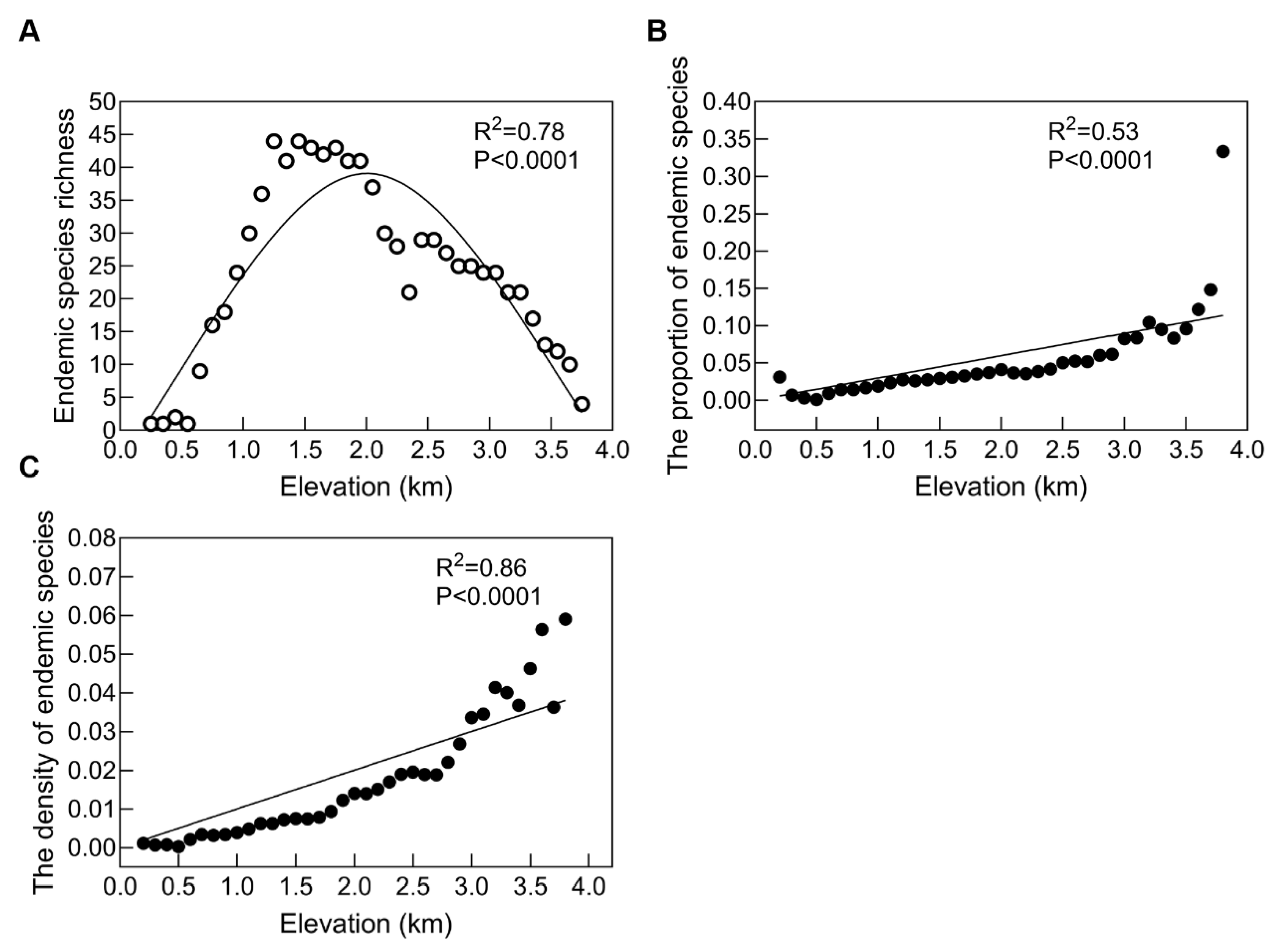
Species richness of seed plants along an altitudinal gradient in the Qinling Mountains showed a single peak, occurring at 1000–1500 m (Figure 1, R2 = 0.67, p < 0.001). Similar patterns were also observed at the genus (Figure 1, R2 = 0.71, p < 0.0001) and family level (Figure 1, R2 = 0.84, p < 0.0001). Species richness of seed plants was first increased and then decreased with the increase of altitude, and it displayed similar trends for three levels (species, genus, and family). After logarithmic corrections to the data at species, genus, and family levels, the goodness of fit was significantly improved (R2 = 0.91, p < 0.001). Endemic species richness in the Qinling Mountains also exhibited a single peak pattern, and the peak was at 1200–2000 m altitude (Figure 2A, R2 = 0.78, p < 0.001). However, the proportion and density of endemic species increased monotonously with altitude (Figure 2B,C). The proportion of endemic species was significantly affected by altitude (Figure 2B, R2 = 0.53, p < 0.001). The higher the altitude, the higher the specificity, which was clearly affected by area. There was an obvious positive correlation between the density of endemic species and altitude (Figure 2C, R2 = 0.86, p < 0.001).

3.2. Explanation of Altitudinal Patterns of Species Richness in Qinling Mountains by Different Hypotheses

3.2.1. Species–Area Relationship Hypothesis

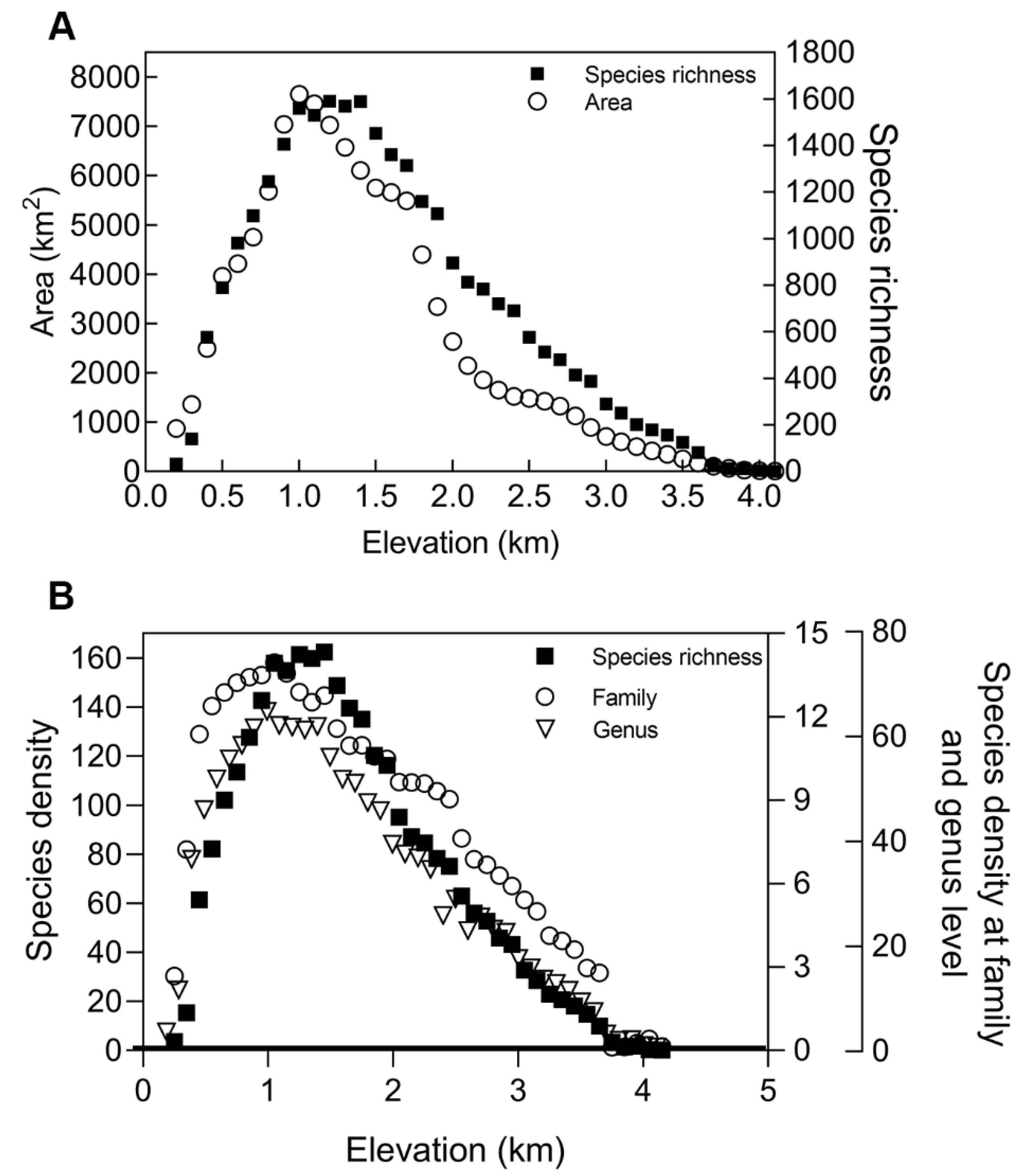
The area showed a single-peak curve pattern along the altitudinal gradient with a peak value of 1000–1500 m (7650 km2). The trend of species richness was the same with the area: species richness increased with altitude below 1000 m; at 1000–1500 m, although the area decreased gradually, the species richness remained at a high level (about 1568 species); above 1500 m, species richness decreased with the altitude (Figure 3A). In order to eliminate the influence of area on the patterns of species richness, the changes of species density at species, genus, and family levels were calculated. Species density at three levels demonstrated a similar off-peak relationship along a coastal gradient, and the peak value tended to the low altitude. At a species level, the peak of species density was at 1200–1500 m; at genus level, the peak appeared at 900–1500 m; at family level, the peak was at 700–1300 m (Figure 3B). The fitting results of the data curve were the same as the altitudinal patterns of species richness at three levels.

3.2.2. The Mid-Domain Effect Hypothesis

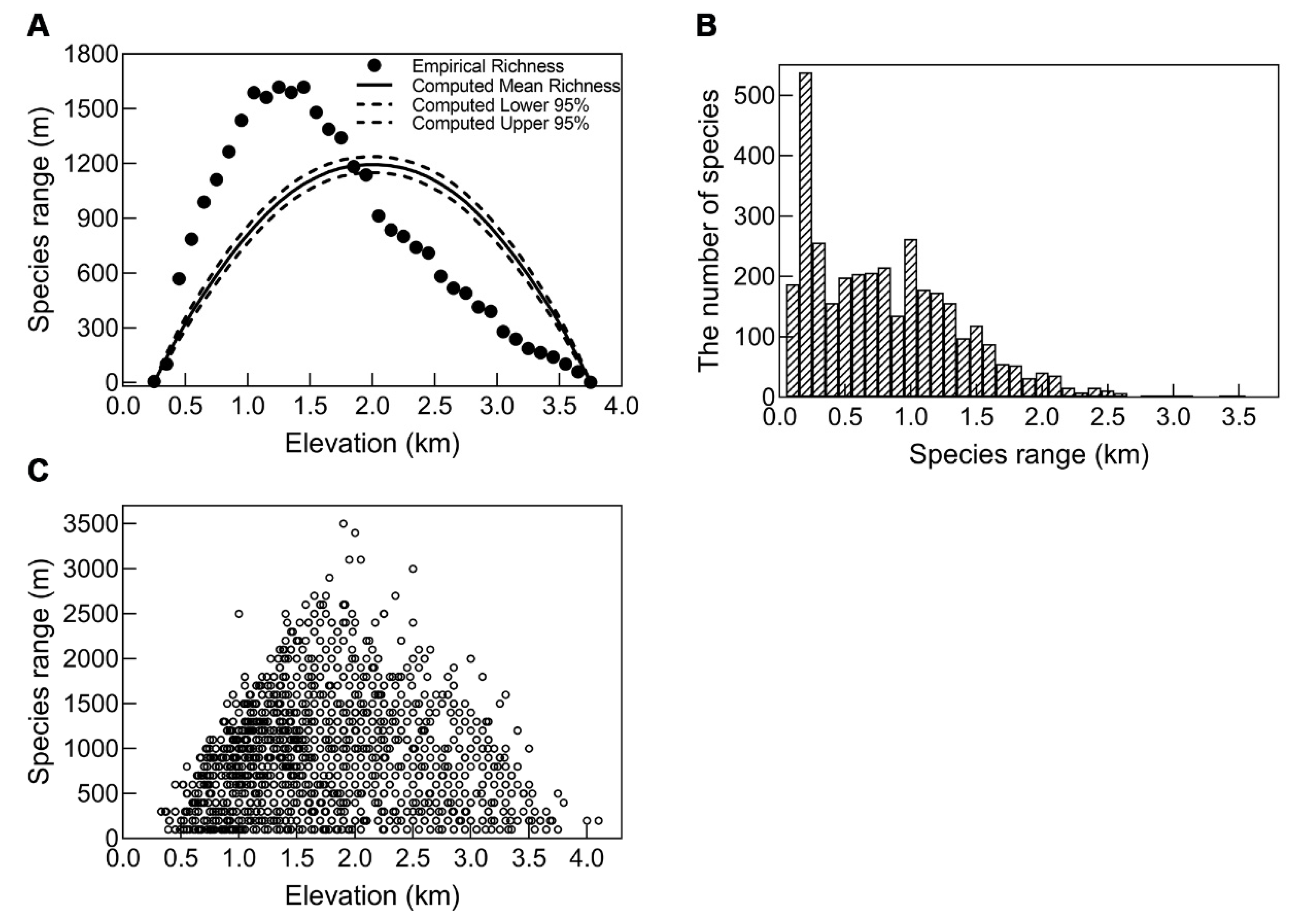
According to the Range model, the maximum species richness of seed plants was 1194, which occurred at 1900–2000 m, but the actual size and peak location of species richness were lower than the predicted value (Figure 4A). The range of species domain was mostly less than 1000 m, accounting for 68.24% of the total species. A total of 538 species were in the range of 200 m, accounting for 15.57% (Figure 4B). The species domain range was unimodal along the altitude gradient, and the region of middle-altitude species was the largest; high-altitude and low-altitude regions were narrow due to the limitation of species diffusion (Figure 4C).

3.2.3. Explanatory Quantity of Different Hypotheses

If only one of the three hypotheses was used to explain species richness, the interpretation of SAR was 69%, MTE was 14.3%, and MDE alone was 79.4% (Table 1). According to the covariance analysis, the interpretation amount of SAR and MTE was 95.9%, that of SAR and MDE was 87.1%, and MTE and MDE was 97.6%. Combining the three hypotheses, the interpretation amount was as high as 98.9%, which could explain most of the changes in species diversity (Table 1).
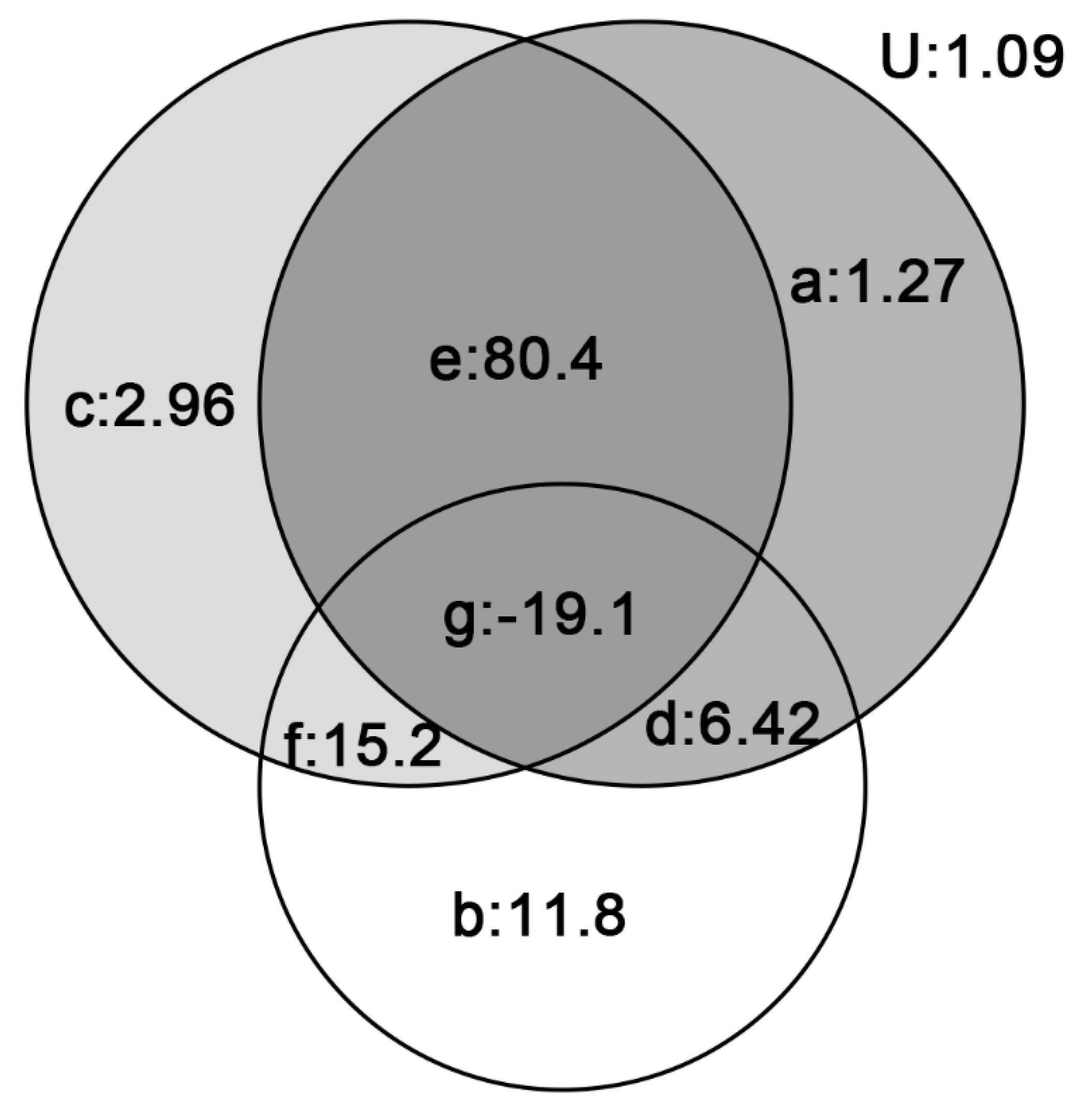
Single-factor fitting could only understand the applicability of the single hypothesis to the altitudinal patterns of species richness in the Qinling Mountains, and which were disturbed by other factors. When the independent contributions of the three hypotheses were calculated by variance separation and multiple stepwise regression, the independent explanatory amounts of SAR, MDE, and MTE were 1.27%, 2.96%, and 11.8%, respectively. When SAR and MDE were combined, the common explanatory amount reached 80.4% (Figure 5), indicating that area and mid-domain effect significantly affect the patterns of plant species richness in the Qinling Mountains.

3.3. A Test of Rapoport’s Rule with Altitude

3.3.1. A Test of Rapoport’s Rule by Four Methods

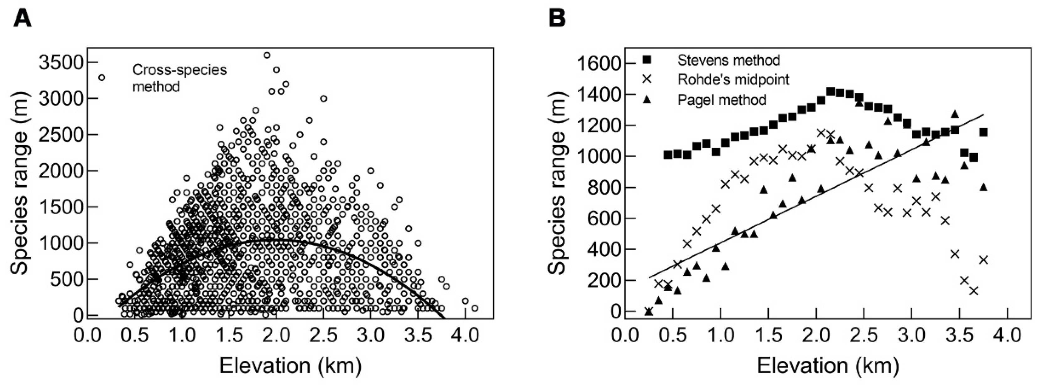
The results of the species-by-species method showed that the species domain distribution range was significantly correlated with altitude. With the increase in altitude, the species domain range first increased and then decreased, belonging to a single peak pattern (Figure 6A, R2 = 0.14, p < 0.0001); all species within each altitude gradient at 400–3800 m were counted by the Stevens method, and the distribution range of species increased along the elevation exhibiting a single peak at 2000–2100 m. Among them, the high data error was at low altitude and high altitude (above 3800 m) (Figure 6B, R2 = 0.76, p < 0.0001). According to the Rohde midpoint method, the distribution range of species of each altitude gradient also demonstrated a single peak pattern, with the peak at 2000–2100 m, while the vertical distributed amplitudes of these species had large differences (Figure 6B, R2= 0.89, p < 0.0001). The Pagel upper limit method was used to display all species at the upper limit of the distribution range along the altitude. Below 3800 m, the domain range increased monotonically with altitude (Figure 6B, R2 = 0.68, p < 0.0001). There were many errors because few species data were above 3800 m.

3.3.2. A Test of Rapoport’s Rule by Grouping Method

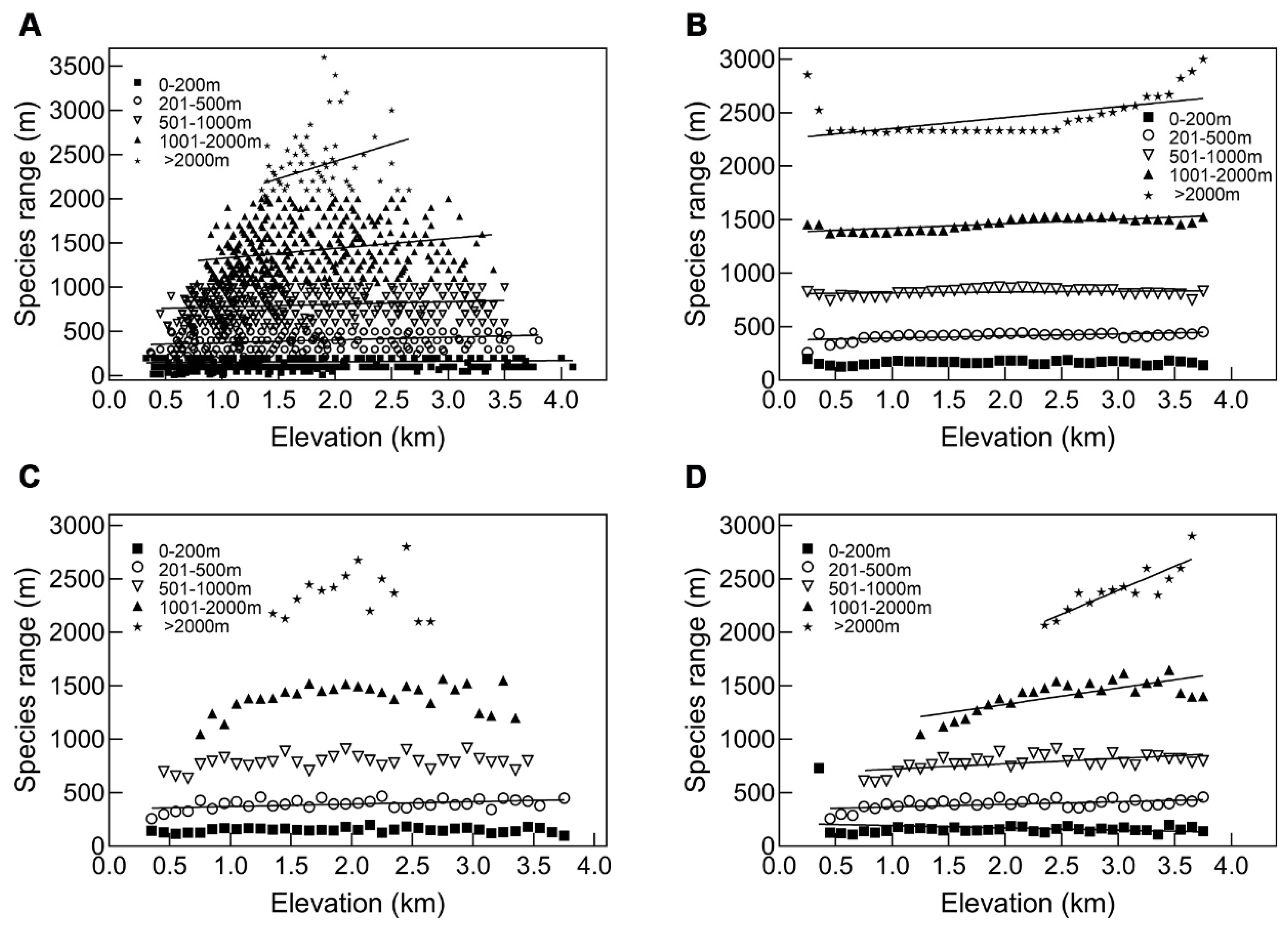
After grouping, the results of the species domain distribution range using the species-by-species method are: 0–200 m (R2 = 0.25, p < 0.0001), 201–500 m (R2 = 0.0337, p < 0.0001), 501–1000 m (R2 = 0.0157, p < 0.001), 1001–2000 m (R2 = 0.081, p < 0.0001), and above 2000 m (R2 = 0.011, p < 0.01). The species domain range of each group increased monotonously with altitude (Figure 7A). In the Stevens method after grouping, there was no significant difference at 0–200 m due to the dispersion of data. The species range at 201–500 m (R2 = 0.325, p < 0.001), 501–1000 m (R2 = 0.167, p < 0.01), 1001–2000 m (R2 = 0.67, p < 0.0001), and above 2000 m (R2 = 0.405, p < 0.0001) increased monotonically along the altitude (Figure 7B). After grouping, the results of the Rohde midpoint method were not ideal. The species range of 0–200 m, 501–1000 m (R2 = 0.082, p = 0.06), 1001–2000 m (R2 = 0.049, p = 0.14), and above 2000 m had little correlation with altitude, and only 201–500 m (R2 = 0.2, p < 0.005) monotonically increased with the elevation (Figure 7C). After grouping, the statistical results of the Pagel upper-bound method showed that the species distribution range had no significant relationship with altitude of 0–200 m, and the data were scattered and the goodness of fit was not high. The species domain range of 201–500 m (R2 = 0.279, p < 0.001), 501–1000 m (R2 = 0.398, p < 0.0001), 1001–2000 m (R2 = 0.589, p < 0.001), and above 2000 m (R2 = 0.815, p < 0.0001) increased significantly with altitude, and the goodness of fit increased gradually (Figure 7D).

4. Discussion and Conclusions

4.1. Species Richness along an Altitudinal Gradient in Qinling Mountains and the Explanatory Power of Different Hypotheses

The species richness of vascular plants showed a hump-shaped pattern along the elevational gradient in the Gyirong Valley [26]; Namgail et al. [27] found a unimodal relationship between plant species richness and altitude at a single mountain as well as at the scale of the entirety of Ladakh. The results in this study were consistent with previous studies: the species richness along the altitude gradient in the Qinling Mountains presented a unimodal pattern, with the maximal being at 1000–1500 m. It showed a similar trend at three classification levels (species, genus, and family) in different altitude gradients. Considering the area, species density at three levels demonstrated a similar off-peak, and the peak tended to the low altitude (below 1500 m). There were many possible reasons for exhibiting a unimodal pattern with a single peak of species richness. These can be grouped into three categories: historical hypotheses invoking processes occurring across evolutionary time scales [28], climatic hypotheses based on current abiotic conditions [29], and spatial hypotheses of area and spatial constraint (mid-domain effect) [30,31,32,33]. In this paper we examined the two spatial hypotheses to which elevational diversity may be responding: (1) climatic hypotheses, (2) spatial hypotheses, and their combined effect. The results showed that the single hypothesis could not fully explain the pattern of species richness on the altitudinal gradient of the Qinling Mountains. The pattern was affected by a variety of factors, of which SAR and MDE account for 80.4%. It shows that area and spatial constraints may be the main factors affecting the altitude pattern of species richness in the Qinling Mountains. The comprehensive effects of area and spatial constraint determine most of the changes in species richness; that is, the spatial hypothesis is more suitable to explain the vertical distribution pattern of plant diversity in the Qinling Mountains.

4.2. Endemic Species Richness Patterns along an Altitudinal Gradient in Qinling Mountains

Endemic species are closely related to biodiversity conservation, but there are few studies on the altitudinal pattern of endemic species richness [34]. Species richness and the proportion of endemic species of all species were found to be related to altitude in Ecuador and Crete [35,36]. The results in this study also showed that the percentage and density of endemic species in Qinling Mountains increased monotonously with altitude, which may be due to three reasons: (I) isolation increases with altitude, and vulnerability is weakly but significantly correlated with both altitude and isolation [37,38]; (II) the survival area of species decreases gradually with altitude, which can cause population fragmentation, and local population is fragmented, accelerating differentiation between species [39]; (III) the formation of endemic species is closely related to climate change, which can act as an evolutionary filter. Species adapted to the existed climate change usually have a wider altitudinal range [40,41].

4.3. A Test of Rapoport’s Rule

In this paper, a variety of methods were used to test whether the altitudinal pattern of seed plant species in the Qinling Mountains conformed to Rapoport’s rule. Only the Pagel upper-bound method supported this law. For all gradients and species within the species domain, the range of species domain increased monotonously along the altitude, which was consistent with the previous research [42,43]. When considering the upper limit of altitudinal distribution of both narrow and wide species, the error would lead to more high-altitude species [44,45]. In Rapoport’s rule, the species that live at high altitudes had a wide range of climate tolerance and wider distribution. In the species-by-species method, the Rhode midpoint method, and the Stevens method, the species domain range showed a single peak pattern along the altitude, which generally did not support Rapoport’s rule in this area. However, all species were grouped according to their altitude distribution, the medium domain effect was partially eliminated, and the grouping test reflected the linear trend in Rapoport’s rule.

5. Conclusions

To sum up, the data used in this study are based on the floristic database. Although the contents of the data are sufficient, there may be some errors, especially in the altitude range of species distribution, and the data that come from the collected samples may affect the accuracy and applicability of the results. The test of Rapoport’s law is obviously affected by the test method, so more advanced and universal methods are expected to be developed in future.

Author Contributions

Conceptualization, Q.L. and M.Y.; methodology, Q.L.; software, T.L.; validation, Q.L., T.L. and M.Y.; formal analysis, Q.L.; investigation, Q.L. and T.L.; resources, Q.L.; data curation, Q.L.; writing—original draft preparation, Q.L.; writing—review and editing, Q.L.; visualization, Q.L.; supervision, M.Y.; project administration, M.Y.; funding acquisition, M.Y. All authors have read and agreed to the published version of the manuscript.

Funding

This research was funded by the Biodiversity Investigation and Evaluation Project of the Ministry of Ecological Environment (2019HJ2096001006), the Scientific and Technological Innovation Project of Shaanxi Forestry Academy of Sciences (SXLK2020-0203), the Ministry of Science and Technology, China (2019FY202300) and Key Project of Shaanxi Academy of Sciences (2020K-05).

Institutional Review Board Statement

Not applicable.

Informed Consent Statement

Not applicable.

Data Availability Statement

The processed data required to reproduce these findings cannot be shared at this time as the data also forms part of an ongoing study.

Acknowledgments

We wish to thank our colleagues for their help. A special thanks to Yuchao Wang, Zhuxin Mao and Yang Li for field work. We are grateful to two reviewers for their constructive comments, which helped us to improve the manuscript.

Conflicts of Interest

The authors declare no conflict of interest.

References

  1. Thiel-Egenter, C.; Gugerli, F.; Alvarez, N.; Brodbeck, S.; Colli, L. Effects of species traits on the genetic diversity of high-mountain plants: A multi-species study across the Alps and the Carpathians. Glob. Ecol. Biogeogr. 2010, 18, 78–87. [Google Scholar] [CrossRef]
  2. Jiang, S.; Kong, F.H.; Hu, R.; Zhang, J.X.; Zhang, M.H. Effects of the climatic region on richness correlations between vascular plants and vertebrates in nature reserves of China. Diversity 2022, 14, 499. [Google Scholar] [CrossRef]
  3. Bradshaw, A.D. Evolutionary significance of phenotypic plasticity in plants. Adv. Genet. 1965, 13, 115–155. [Google Scholar]
  4. Leopold, C.R.; Hess, S.C. Facilitating adaptation to climate change while restoring a montane plant community. PLoS ONE 2019, 14, e218516. [Google Scholar] [CrossRef] [PubMed] [Green Version]
  5. Gaston, K.J. Global patterns in biodiversity. Nature 2000, 405, 220–227. [Google Scholar] [CrossRef]
  6. Acharya, B.K.; Chettri, B.; Vijayan, L. Distribution pattern of trees along an elevation gradient of Eastern Himalaya, India. Acta Oecol. 2011, 37, 329–336. [Google Scholar] [CrossRef]
  7. Gurvich, D.E.; Zeballos, S.R.; Demaio, P.H. Diversity and composition of cactus species along an altitudinal gradient in the Sierras del Norte Mountains (Cordoba, Argentina). S. Afr. J. Bot. 2014, 93, 142–147. [Google Scholar] [CrossRef] [Green Version]
  8. Shimwell, D.W. Areography. Geographical Strategies of Species. by E. H. Rapoport. J. Ecol. 1983, 71, 1037–1038. [Google Scholar] [CrossRef]
  9. Rapoport, E.H. Ecological Areography. In Areography; Elsevier: Amsterdam, The Netherlands, 1982; pp. 210–241. [Google Scholar]
  10. Stevens, G.C. The latitudinal gradient in geographical range: How so many species coexist in the tropics. Am. Nat. 1989, 133, 240–256. [Google Scholar] [CrossRef]
  11. Stevens, G.C. The elevational gradient in altitudinal range: An extension of Rapoport’s latitudinal rule to altitude. Am. Nat. 1992, 140, 893–911. [Google Scholar] [CrossRef]
  12. Egoh, B.; Reyers, B.; Rouget, M.; Bode, M.; Richardson, D.M. Spatial congruence between biodiversity and ecosystem services in South Africa. Biol. Conserv. 2009, 142, 553–562. [Google Scholar] [CrossRef]
  13. Lee, P.Y.; Rotenberry, J.T. Relationships between bird species and tree species assemblages in forested habitats of eastern North America. J. Biogeogr. 2010, 32, 1139–1150. [Google Scholar] [CrossRef]
  14. Fady, B.; Conord, C. Macroecological patterns of species and genetic diversity in vascular plants of the Mediterranean Basin. Divers. Distrib. 2009, 16, 53–64. [Google Scholar] [CrossRef]
  15. Li, X.; Tian, H.; Wang, Y.; Li, R.; Song, Z.; Zhang, F.; Xu, M.; Li, D. Vulnerability of 208 endemic or endangered species in China to the effects of climate change. Reg. Environ. Chang. 2013, 13, 843–852. [Google Scholar] [CrossRef]
  16. Araújo, M.B.; Rahbek, C. How does climate change affect biodiversity? Science 2006, 313, 1396–1397. [Google Scholar] [CrossRef]
  17. Heikkinen, R.K.; Kartano, L.; Leikola, N.; Aalto, J.; Virkkala, R. High-latitude EU habitats directive species at risk due to climate change and land use. Glob. Ecol. Conserv. 2021, 28, e1664. [Google Scholar] [CrossRef]
  18. Panitsa, M.; Trigas, P.; Iatrou, G.; Sfenthourakis, S. Factors affecting plant species richness and endemism on land-bridge islands—An example from the East Aegean archipelago. Acta Oecol. 2010, 36, 431–437. [Google Scholar] [CrossRef]
  19. Trigas, P.; Iatrou, G.; Panitsa, M. Vascular plant species diversity, biogeography and vulnerability in the aegean islands as exemplified by Evvia Island (W Aegean, Greece). Fresen. Environ. Bull. 2015, 17, 48–57. [Google Scholar]
  20. Gehrke, B.; Linder, H.P. Species richness, endemism and species composition in the tropical Afroalpine flora. Alp. Bot. 2014, 124, 165–177. [Google Scholar] [CrossRef]
  21. Lamoreux, J.F.; Morrison, J.C.; Ricketts, T.H.; Olson, D.M.; Dinerstein, E.; McKnight, M.W.; Shugart, H.H. Global tests of biodiversity concordance and the importance of endemism. Nature 2006, 440, 212–214. [Google Scholar] [CrossRef] [PubMed]
  22. Sharma, S.; Legendre, P.; Boisclair, D.; Gauthier, S.; Smith, S.J. Effects of spatial scale and choice of statistical model (linear versus tree-based) on determining species-habitat relationships. Can. J. Fish. Aquat. Sci. 2012, 69, 2095–2111. [Google Scholar] [CrossRef]
  23. Chi, X.; Tang, Z. Effects of area, temperature and geometric constraints on elevational patterns of species richness:a case study in the Mountain Taibai, Qinling Mountains, China. Chin. J. Plant Ecol. 2011, 35, 362–370. [Google Scholar] [CrossRef]
  24. Yue, M.; Zhang, L.; Dang, G.; Tian, G.U. The relationships of higher plants diversity and elevation gradient in Foping National Reserve. Sci. Geogr. Sin. 2002, 22, 349–354. [Google Scholar]
  25. Fu, Z.; Zhang, X.; Shunyi, L.; Ming, T. The summarize of research on the flora and vegetation of the Qinling Mountain range. Acta Bot. Boreall.-Occident. Sin. 1996, 16, 93–106. [Google Scholar]
  26. Liang, J.; Ding, Z.; Lie, G.; Zhou, Z.; Hu, Z. Species richness patterns of vascular plants and their drivers along an elevational gradient in the central Himalayas. Glob. Ecol. Conserv. 2020, 24, e01279. [Google Scholar] [CrossRef]
  27. Namgail, T.; Rawat, G.S.; Mishra, C.; Van Wieren, S.E.; Prins, H.H.T. Biomass and diversity of dry alpine plant communities along altitudinal gradients in the Himalayas. J. Plant Res. 2012, 125, 93–101. [Google Scholar] [CrossRef] [Green Version]
  28. Mittelbach, G.G.; Schemske, D.W.; Cornell, H.V.; Allen, A.P.; Brown, J.M.; Bush, M.B.; Harrison, S.P.; Hurlbert, A.H.; Knowlton, N.; Lessios, H.A. Evolution and the latitudinal diversity gradient: Speciation, extinction and biogeography. Ecol. Lett. 2007, 10, 315–331. [Google Scholar] [CrossRef]
  29. Hawkins, B.A.; Diniz-Filho, J.A.; Jaramillo, C.A.; Soeller, S.A. Climate, niche conservatism, and the global bird diversity gradient. Am. Nat. 2007, 170 (Suppl. S2), S16–S27. [Google Scholar] [CrossRef] [PubMed]
  30. Terborgh, J. On the notion of favorableness in plant ecology. Am. Nat. 1973, 107, 481–501. [Google Scholar] [CrossRef]
  31. Rosenzweig, M.L. Species Diversity Gradients: We know more and less than we thought. J. Mammal. 1992, 73, 715–730. [Google Scholar] [CrossRef]
  32. Colwell, R.K.; Rahbek, C.; Gotelli, N.J. The middomain effect and species richness patterns: What have we learned so far? Am. Nat. 2004, 163, E1–E23. [Google Scholar] [CrossRef] [PubMed] [Green Version]
  33. Cardelus, C.L.; Colwell, R.K.; Watkins, J.E. Vascular epiphyte distribution patterns: Explaining the mid-elevation richness peak. J. Ecol. 2006, 94, 144–156. [Google Scholar] [CrossRef]
  34. Trigas, P.; Panitsa, M.; Tsiftsis, S. Elevational gradient of vascular plant species richness and endemism in Crete—The effect of Post-Isolation mountain uplift on a continental island system. PLoS ONE 2013, 8, e59425. [Google Scholar] [CrossRef] [PubMed]
  35. Kessler, M. The elevational gradient of Andean plant endemism: Varying influences of taxon-specific traits and topography at different taxonomic levels. J. Biogeogr. 2002, 29, 1159–1165. [Google Scholar] [CrossRef]
  36. Colwell, R.K. RangeModel: Tools for exploring and assessing geometric constraints on species richness (the mid-domain effect) along transects. Ecography 2008, 31, 4–7. [Google Scholar] [CrossRef]
  37. Selvi, E. Rare plants on Mount Amiata, Italy: Vulnerability to extinction on an ecological ‘island’. Biol. Conserv. 1997, 81, 257–266. [Google Scholar] [CrossRef]
  38. González-Suárez, M.; Gómez, A.; Revilla, E. Which intrinsic traits predict vulnerability to extinction depends on the actual threatening processes. Ecosphere 2013, 4, 1–16. [Google Scholar] [CrossRef] [Green Version]
  39. Myers, E.M.; Harwell, T.I.; Yale, E.L.; Lamb, A.M.; Anthony, F.W.; Norman, J. Multifaceted, cross-generational costs of hybridization in sibling Drosophila species. PLoS ONE 2013, 8, e80331. [Google Scholar] [CrossRef] [Green Version]
  40. Inouye, D.W.; Barr, B.; Armitage, K.B.; Inouye, B.D. Climate change is affecting altitudinal migrants and hibernating species. Proc. Natl. Acad. Sci. USA 2000, 97, 1630–1633. [Google Scholar] [CrossRef] [Green Version]
  41. Thomas, C.D. Translocation of species, climate change, and the end of trying to recreate past ecological communities. Trends Ecol. Evol. 2011, 26, 216–221. [Google Scholar] [CrossRef]
  42. Feng, J.; Hu, X.; Wang, J.; Wang, Y. Support for the elevational Rapoport’s rule among seed plants in Nepal depends on biogeographical affinities and boundary effects. Ecol. Evol. 2016, 6, 7246–7252. [Google Scholar] [CrossRef] [PubMed]
  43. Kim, J.D.; Lee, M.H.; Song, J.H.; Byeon, S.Y.; Lee, G.E.; Kim, H.J.; Chae, S.B.; Yun, C.W.; Kim, J.D. Empirical evaluation of the elevational Rapoport’s rule: The species richness patterns for vascular plants on Seorak Mountain, Korea: Relationship between group of life forms and phytogeography affinity along the elevational gradient. Ecol. Evol. 2021, 11, 12872–12881. [Google Scholar] [CrossRef]
  44. Saito, S.; Kato, N.; Kudara, H.; Kagawa, S. Structure and floristic composition of a beech forest at the upper limit of the altitudinal distribution. Bull. Gumma Prefect. Womens Coll. 1983, 3, 115–122. [Google Scholar]
  45. Takahashi, K.; Azuma, H.; Yasue, K. Effects of climate on the radial growth of tree species in the upper and lower distribution limits of an altitudinal ecotone on Mount Norikura, central Japan. Ecol. Res. 2010, 18, 549–558. [Google Scholar] [CrossRef] [Green Version]
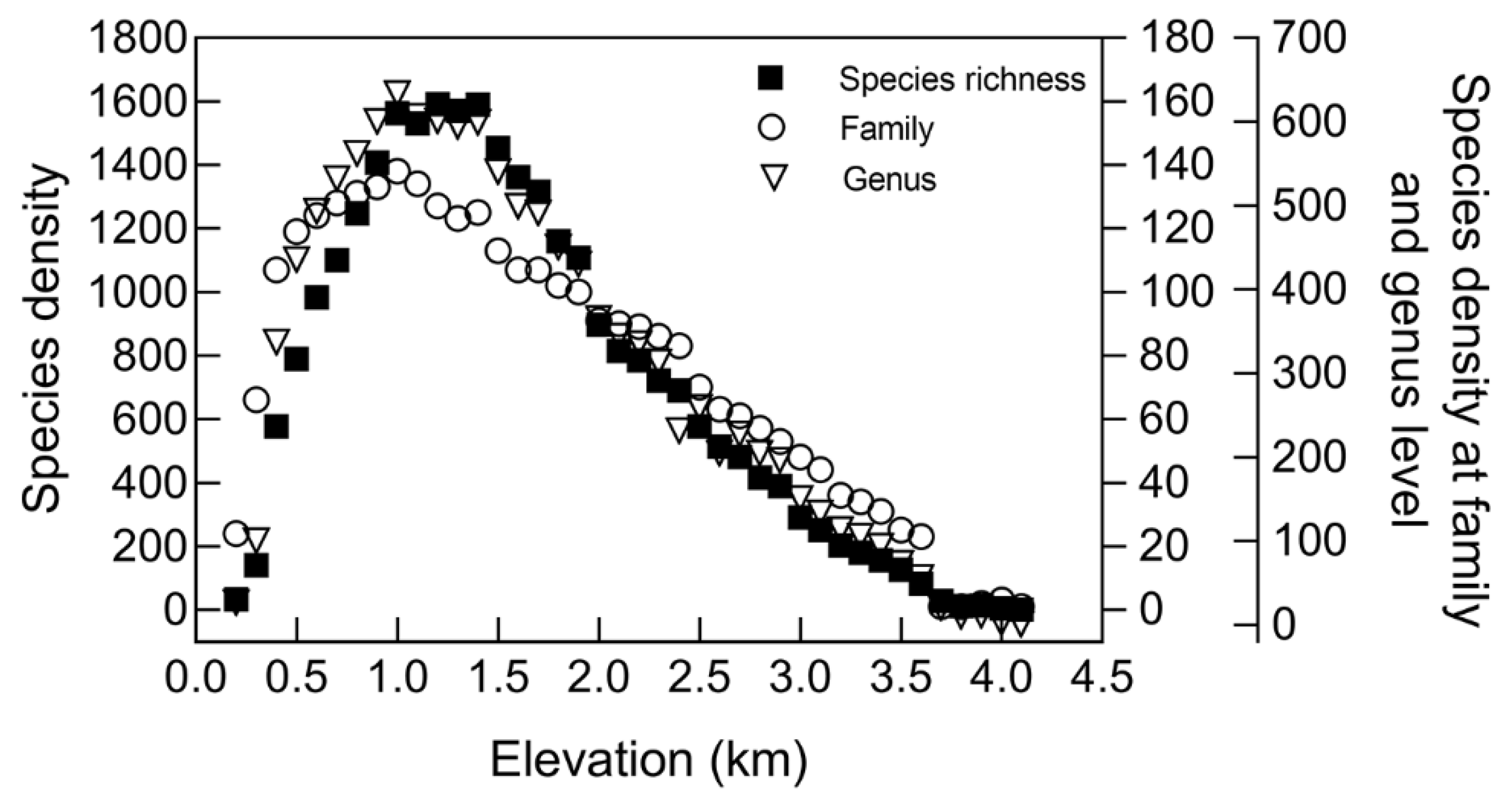
Figure 1. The altitudinal patterns of richness in Qinling Mountains at species (square), genus (inverted triangle), and family (circle) levels.
Diversity 14 00603 g001
Figure 2. (A) The altitudinal patterns of endemic species richness in Qinling Mountains. (B) The proportion of endemic species along an altitudinal gradient. (C) The density of endemic species.
Diversity 14 00603 g002
Figure 3. (A) The altitudinal patterns of species richness and area in Qinling Mountains (B) The altitudinal patterns of density in Qinling Mountains at species (square), genus (inverted triangle), and family (circle) levels.
Diversity 14 00603 g003
Figure 4. (A) The patterns between predicted species richness and actual species richness with elevation by range model. (B) Variation in the number of species in different species range. (C) The patterns of species range with elevation.
Diversity 14 00603 g004
Figure 5. The relative contributions of the three hypotheses to explain the patterns of species richness. a, b, and c represent independent effects of SAR, MTE, and MDE; d, e, and f represent the interactions between them; g represents the combined effect of the three factors and u represents the unexplained quantity.
Diversity 14 00603 g005
Figure 6. (A) The altitudinal patterns of species range in cross-species method. (B) The altitudinal patterns of species range in Stevens methods, Rohde’s midpoint method, and Pagel’s method.
Diversity 14 00603 g006
Figure 7. The altitudinal patterns of species range after grouping in cross-species method (A), Stevens method (B), Rohde’s midpoint method (C), and Pagel’s method (D).
Diversity 14 00603 g007
Table 1. Interpretation of the three hypotheses on the species diversity of seed plants in Qinling Mountains (R2).
HypothesisR2
SAR0.689
MTE0.143
MDE0.794
SAR + MTE0.959
SAR + MDE0.871
MTE + MDE0.976
SAR + MTE + MDE0.989
Publisher’s Note: MDPI stays neutral with regard to jurisdictional claims in published maps and institutional affiliations.