

The Big Five: Species Distribution Models from Citizen Science Data as Tool for Preserving the Largest Protected Saproxylic Beetles in Italy
 , , , and
Abstract
:1. Introduction
2. Materials and Methods
2.1. Occurrence Data
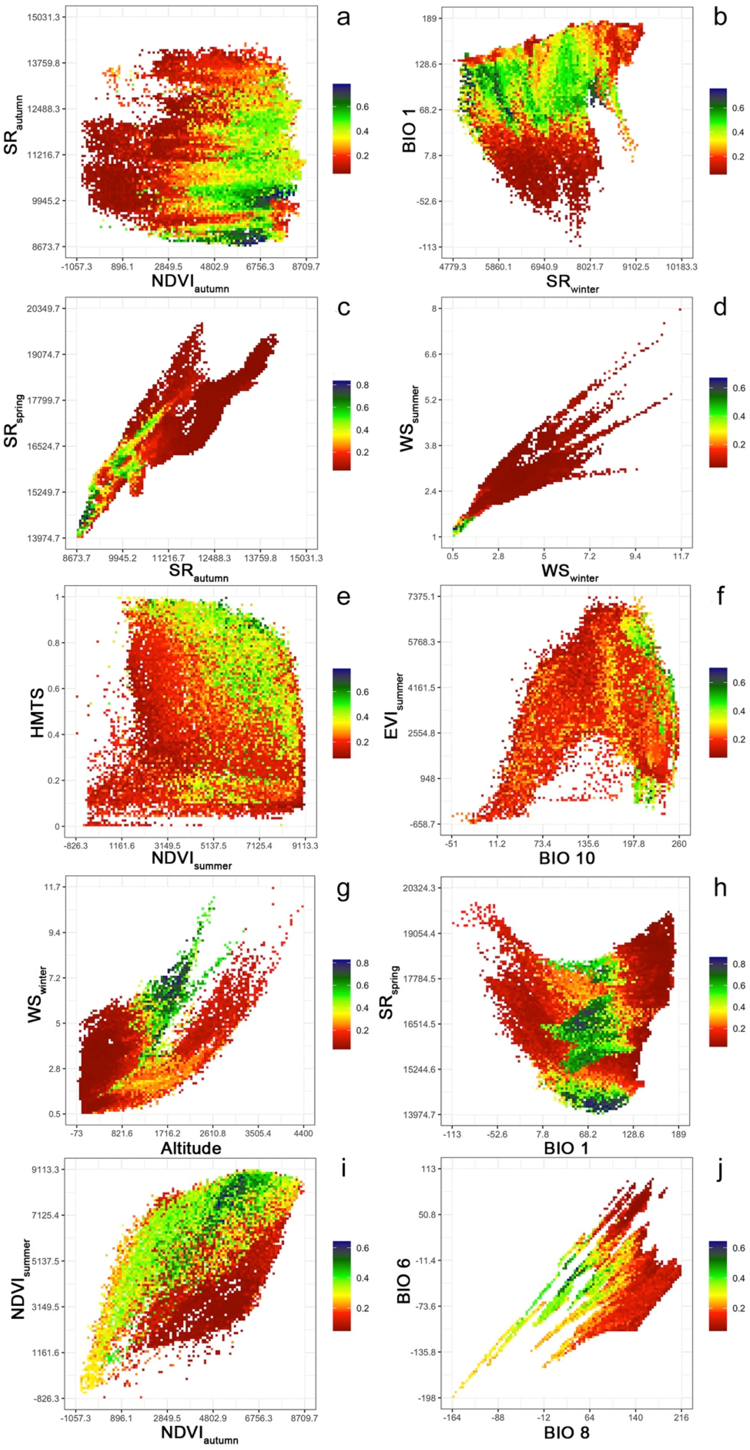
2.2. Environmental Variables Selection
2.3. Species Distribution Model
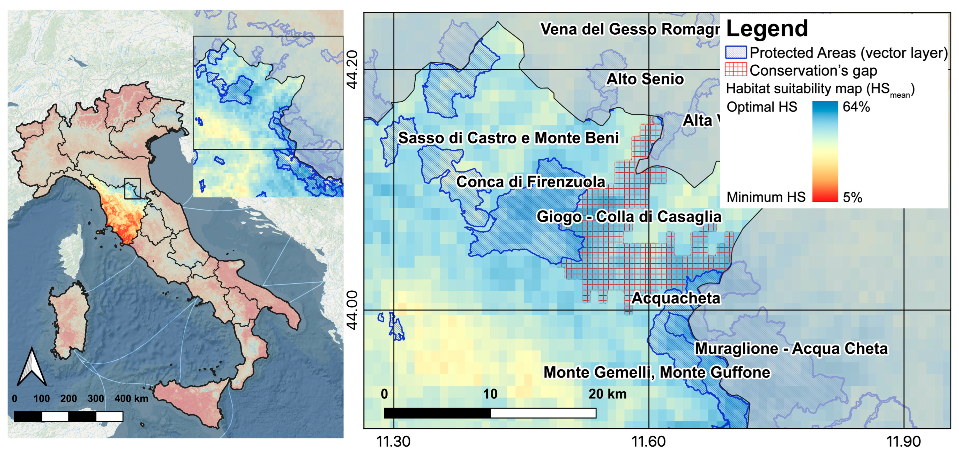
2.4. Gap Analysis
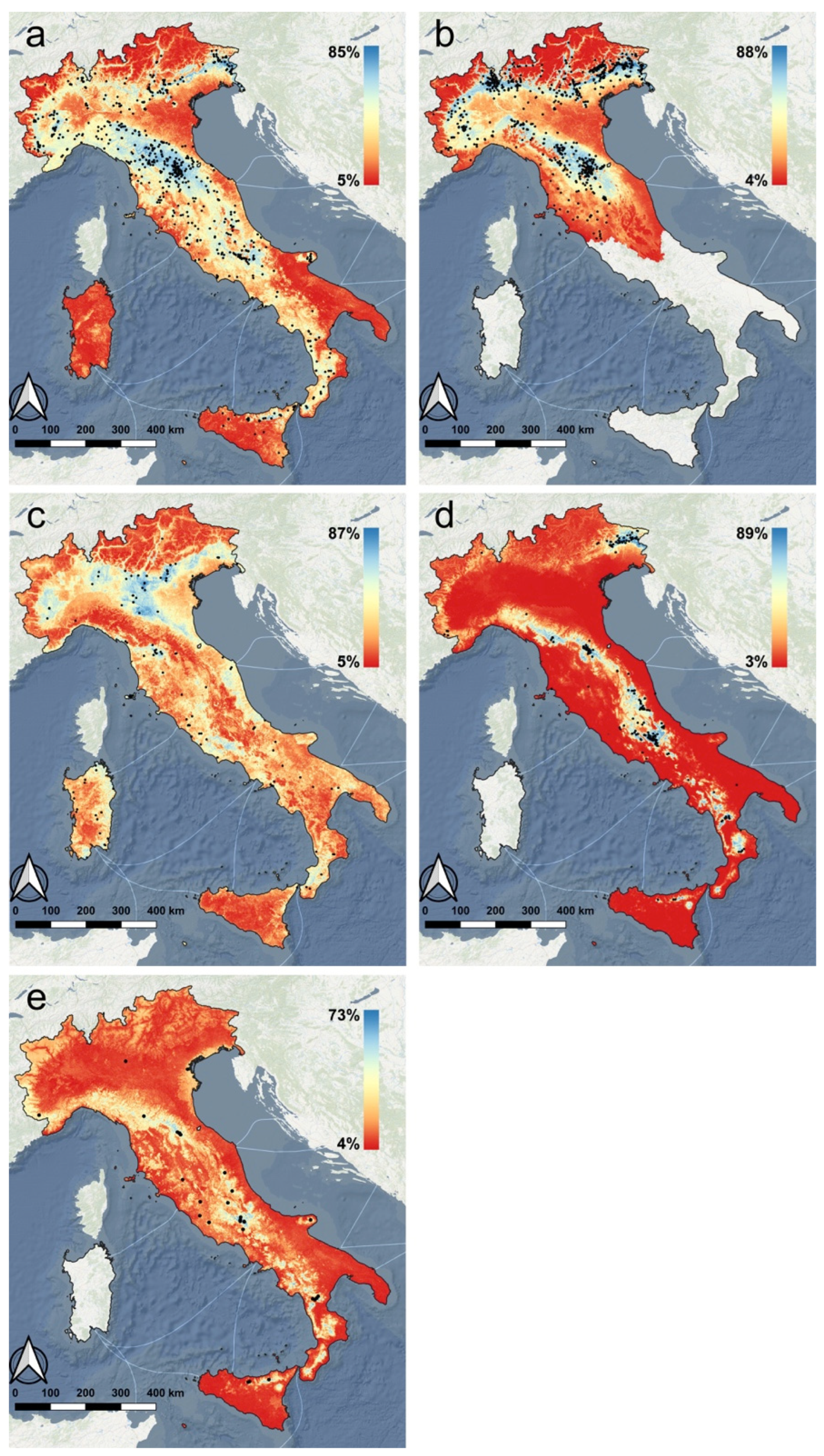
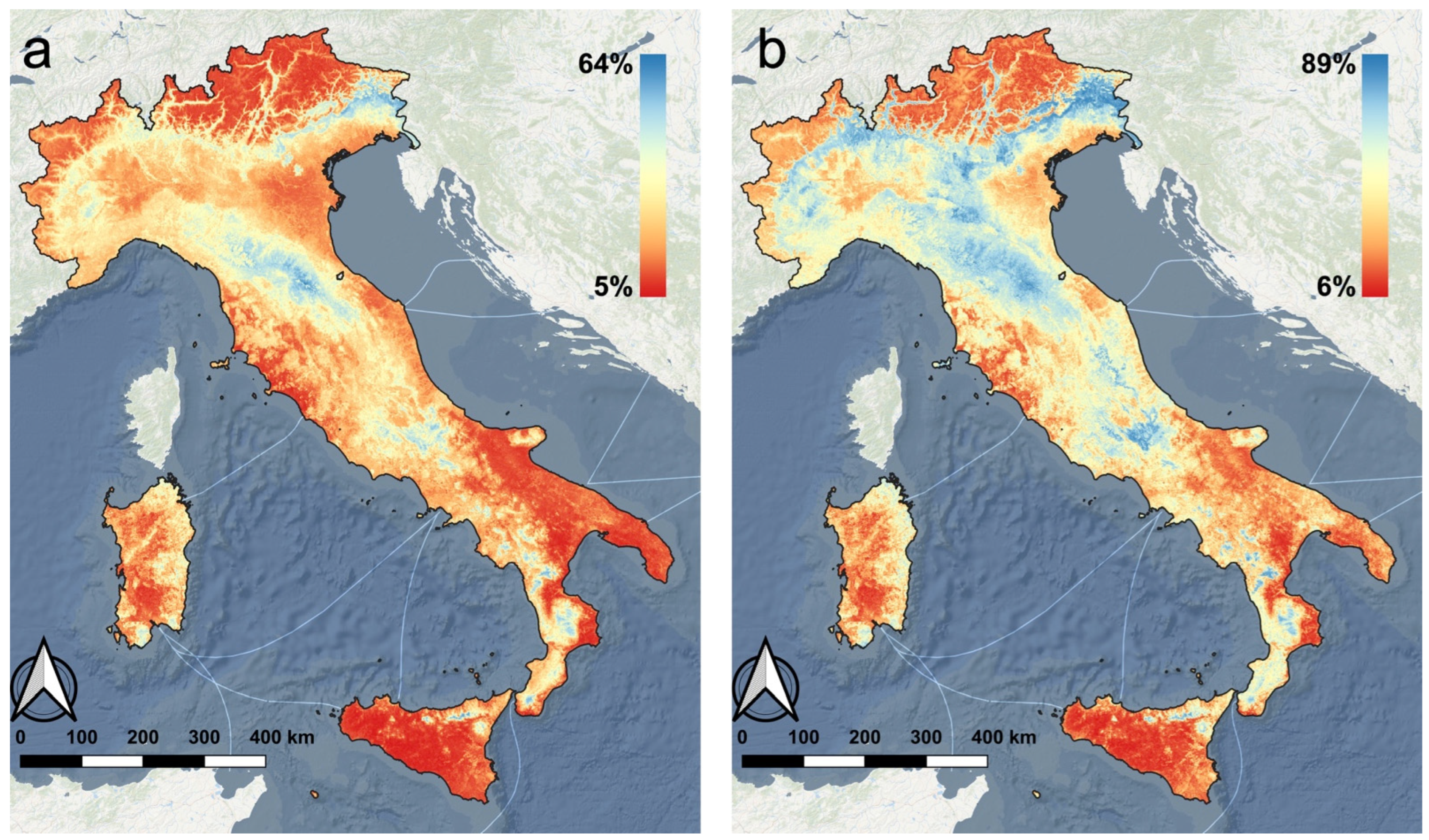
3. Results
3.1. Species Distribution Model
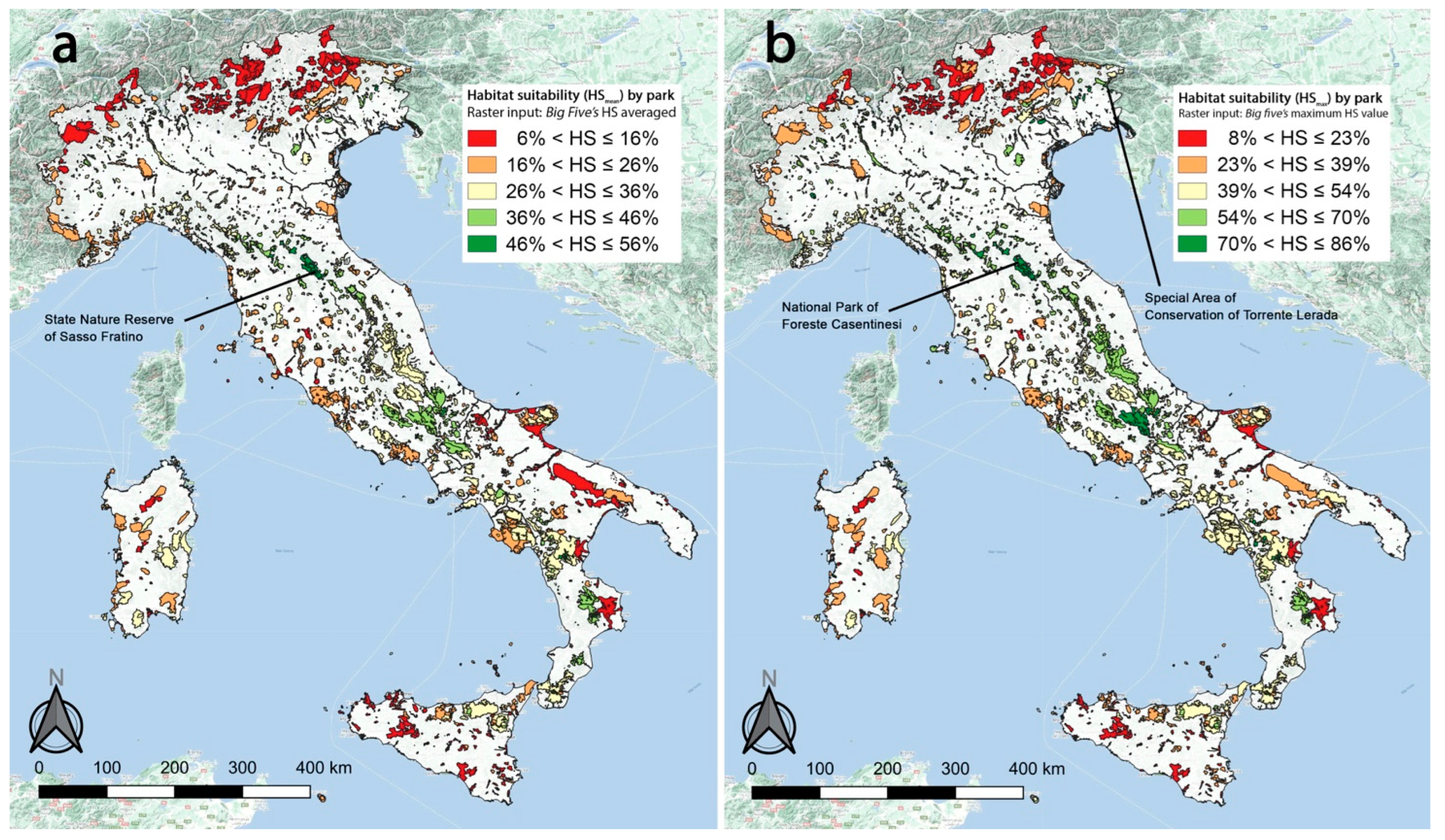
3.2. Gap Analysis
4. Discussion
Supplementary Materials
Author Contributions
Funding
Institutional Review Board Statement
Informed Consent Statement
Data Availability Statement
Acknowledgments
Conflicts of Interest
References
- Feldman, M.J.; Imbeau, L.; Marchand, P.; Mazerolle, M.J.; Darveau, M.; Fenton, N.J. Trends and gaps in the use of citizen science derived data as input for species distribution models: A quantitative review. PLoS ONE 2021, 16, e0234587. [Google Scholar] [CrossRef] [PubMed]
- Cooper, C.B.; Shirk, J.; Zuckerberg, B. The invisible prevalence of citizen science in global research: Migratory birds and climate change. PLoS ONE 2014, 9, e106508. [Google Scholar] [CrossRef] [PubMed] [Green Version]
- Danielsen, F.; Jensen, P.M.; Burgess, N.D.; Altamirano, R.; Alviola, P.A.; Andrianandrasana, H.; Brashares, J.S.; Burton, A.C.; Coronado, I.; Corpuz, N.; et al. Multicountry Assessment of Tropical Resource Monitoring by Local Communities. BioScience 2014, 64, 236–251. [Google Scholar] [CrossRef] [Green Version]
- Gardiner, M.; Allee, L.; Brown, P.M.; Losey, J.E.; Roy, H.E.; Smyth, R.R. Lessons from lady beetles: Accuracy of monitoring data from US and UK citizen-science programs. Front. Ecol. Environ. 2012, 10, 471–476. [Google Scholar] [CrossRef] [Green Version]
- Matutini, F.; Baudry, J.; Pain, G.; Sineau, M.; Pithon, J. How citizen science could improve species distribution models and their independent assessment. Ecol. Evol. 2021, 11, 3028–3039. [Google Scholar] [CrossRef]
- McKinley, D.C.; Miller-Rushing, A.J.; Ballard, H.L.; Bonney, R.; Brown, H.; Cook-Patton, S.C.; Soukup, M.A. Citizen science can improve conservation science, natural resource management, and environmental protection. Biol. Conserv. 2017, 208, 15–28. [Google Scholar] [CrossRef] [Green Version]
- Moreira, F.S.; Regos, A.; Gonçalves, J.F.; Rodrigues, T.M.; Verde, A.; Pérez, J.A.; Meunier, B.; Lepetit, J.-P.; Honrado, J.P.; Gonçalves, D. Combining Citizen Science Data and Satellite Descriptors of Ecosystem Functioning to Monitor the Abundance of a Migratory Bird during the Non-Breeding Season. Remote Sens. 2022, 14, 463. [Google Scholar] [CrossRef]
- Steen, V.A.; Elphick, C.S.; Tingley, M.W. An evaluation of stringent filtering to improve species distribution models from citizen science data. Divers. Distrib. 2019, 25, 1857–1869. [Google Scholar] [CrossRef]
- Hernandez, P.A.; Graham, C.H.; Master, L.L.; Albert, D.L. The effect of sample size and species characteristics on performance of different species distribution modeling methods. Ecography 2006, 29, 773–785. [Google Scholar] [CrossRef]
- Clavero, M.; García-Berthou, E. Invasive species are a leading cause of animal extinctions. Trends Ecol. Evol. 2005, 20, 110. [Google Scholar] [CrossRef] [PubMed]
- Dirzo, R.; Young, H.S.; Galetti, M.; Ceballos, G.; Isaac, N.J.; Collen, B. Defaunation in the anthropocene. Science 2014, 345, 401–406. [Google Scholar] [CrossRef] [PubMed]
- Pimm, S.L.; Raven, P. Extinction by numbers. Nature 2000, 403, 843–845. [Google Scholar] [CrossRef] [PubMed]
- Steffen, W.; Grinevald, J.; Crutzen, P.; McNeill, J. The Anthropocene: Conceptual and historical perspectives. Philos. Trans. R. Soc. A Math. Phys. Eng. Sci. 2011, 369, 842–867. [Google Scholar] [CrossRef] [PubMed]
- Jetz, W.; McPherson, J.M.; Guralnick, R.P. Integrating biodiversity distribution knowledge: Toward a global map of life. Trends Ecol. Evol. 2012, 27, 151–159. [Google Scholar] [CrossRef]
- Silvertown, J. A new dawn for citizen science. Trends Ecol. Evol. 2009, 24, 467–471. [Google Scholar] [CrossRef] [PubMed]
- Zapponi, L.; Cini, A.; Bardiani, M.; Hardersen, S.; Maura, M.; Maurizi, E.; Redolfi De Zan, L.; Audisio, P.; Bologna, M.A.; Carpaneto, G.M.; et al. Citizen science data as an efficient tool for mapping protected saproxylic beetles. Biol. Conserv. 2017, 208, 139–145. [Google Scholar] [CrossRef]
- Speight, M.C.D. Saproxylic Invertebrates and Their Conservation; Council of Europe, Series 46 Publications and Documents Division: Strasbourg, France, 1989. [Google Scholar]
- Lassauce, A.; Paillet, Y.; Jactel, H.; Bouget, C. Deadwood as a surrogate for forest biodiversity: Meta-analysis of correlations between deadwood volume and species richness of saproxylic organisms. Ecol. Indic. 2011, 11, 1027–1039. [Google Scholar] [CrossRef]
- Pechacek, P.; Kristin, A. Comparative diets of adult and young threetoed woodpeckers in a European alpine forest community. J. Wildl. Manag. 2004, 68, 683–693. [Google Scholar] [CrossRef]
- Stokland, J.N. The Saproxylic Food Web. Biodiversity in Dead Wood; Stokland, J.N., Siitonen, J., Jonsson, B.G., Eds.; Cambridge University Press: New York, NY, USA, 2012; pp. 29–54. [Google Scholar]
- Dollin, P.E.; Majka, C.G.; Duinker, P.N. Saproxylic beetle (Coleoptera) communities and forest management and practices in coniferous stands in southwestern Nova Scotia, Canada. Zookeys 2008, 2, 291–336. [Google Scholar]
- Buse, J.; Ranius, T.; Assmann, T. An endangered longhorn beetle associated with old oaks and its possible role as an ecosystem engineer. Conserv. Biol. 2008, 22, 329–337. [Google Scholar] [CrossRef]
- Duelli, P.; Wermelinger, B. Rosalia alpina L.: Un Cerambicide raro ed emblematico. Sherwood 2005, 114, 19–23. [Google Scholar]
- Lachat, T.; Ecker, K.; Duelli, P.; Wermelinger, B. Population trends of Rosalia alpina (L.) in Switzerland: A lasting turnaround? J. Insect Conserv. 2013, 17, 653–662. [Google Scholar] [CrossRef]
- Rink, M.; Sinsch, U. Radio-telemetric monitoring of dispersing stag beetles: Implications for conservation. J. Zool. 2007, 272, 235–243. [Google Scholar] [CrossRef]
- Russo, D.; Cistrone, L.; Garonna, A.P. Habitat selection in the highly endangered beetle Rosalia alpina: A multiple spatial scale assessment. J. Insect Conserv. 2011, 15, 685–693. [Google Scholar] [CrossRef]
- Audisio, P.; Baviera, C.; Carpaneto, G.M.; Biscaccianti, A.B.; Battistoni, A.; Teofili, C.; Rondinini, C. Lista Rossa IUCN dei Coleotteri saproxilici Italiani; Comitato Italiano IUCN e Ministero dell’Ambiente e della Tutela del Territorio e del Mare: Rome, Italy, 2014. [Google Scholar]
- Stoch, F. CK2000. Checklist of the Species of the Italian Fauna. Online Version 2.1. 2003. Available online: https://www.faunaitalia.it/checklist/ (accessed on 15 March 2021).
- Danilevsky, M.L. A new species of the genus Morimus Brullé, 1832 (Coleoptera, Cerambycidae) from Central Europe. Humanit. Space Int. Alm. 2015, 4, 215–219. [Google Scholar]
- Danilevsky, M.L.; Gradinarov, D.; Sivilov, O. A new subspecies of Morimus verecundus (Faldermann, 1836) from Bulgaria and a new subspecies of Morimus asper (Sulzer, 1776) from Greece (Coleoptera, Cerambycidae). Humanit. Space Int. Alm. 2016, 5, 187–191. [Google Scholar]
- Bense, U. Longhorn Beetles: Illustrated key to the Cerambycidae and Vesperidae of Europe; Margraf Verlag: Weikersheim, Germany, 1995. [Google Scholar]
- Hardersen, S.; Cuccurullo, A.; Bardiani, M.; Bologna, M.A.; Mason, F.; Maura, M.; Maurizi, E.; Roversi, P.F.; Sabbatini Peverieri, G.; Chiari, S. Monitoring the saproxylic longhorn beetle Morimus asper-investigating wood characteristics, season, time of the day and odour traps. J. Insect Conserv. 2017, 21, 231–242. [Google Scholar] [CrossRef]
- Bardiani, M.; Chiari, S.; Maurizi, E.; Tini, M.; Toni, I.; Zauli, A.; Campanaro, A.; Carpaneto, G.M.; Audisio, P. Guidelines for the monitoring of Lucanus cervus. In Guidelines for the Monitoring of the Saproxylic Beetles protected in Europe; Carpaneto, G.M., Audisio, P., Bologna, M.A., Roversi, P.F., Mason, F., Eds.; Nature Conservation: Sofia, Bulgaria, 2017; Volume 20, pp. 37–78. [Google Scholar]
- Franciscolo, M.E. Coleoptera Lucanidae. Fauna d’Italia; Calderini Edizioni: Bologna, Italy, 1997; Volume XXXV. [Google Scholar]
- Lapiana, F.; Sparacio, I. I Coleotteri Lamellicorni delle Madonie (Sicilia) (Insecta Coleoptera Lucanoidea et Scarabaeoidea). Naturalista siciliano (S. IV) 2006, 30, 227–292. [Google Scholar]
- Romiti, F.; Redolfi De Zan, L.; Piras, P.; Carpaneto, G.M. Shape variation of mandible and head in Lucanus cervus (Coleoptera: Lucanidae): A comparison of morphometric approaches. Biol. J. Linn. Soc. 2017, 120, 836–851. [Google Scholar] [CrossRef]
- Redolfi De Zan, L.; Bardiani, M.; Antonini, G.; Campanaro, A.; Chiari, S.; Mancini, E.; Maura, M.; Sabatelli, S.; Solano, E.; Zauli, A.; et al. Guidelines for the monitoring of Cerambyx cerdo. In Guidelines for the Monitoring of the Saproxylic Beetles protected in Europe; Carpaneto, G.M., Audisio, P., Bologna, M.A., Roversi, P.F., Mason, F., Eds.; Nature Conservation: Sofia, Bulgaria, 2017; Volume 20, pp. 129–164. [Google Scholar]
- Villiers, A. Faune des Coléoptères de France. 1. Cerambycidae; Editions Lechavalier: Paris, France, 1978. [Google Scholar]
- Bense, U.; Klausnitzer, B.; Bussler, H.; Schmidl, J. Rosalia alpina (Linnaeus, 1758) Alpenbock. In Das europäische Schutzgebietssystem Natura 2000; Petersen, B., Ellwanger, G., Biewald, G., Hauke, U., Ludwig, G., Pretscher, P., Schröder, E., Ssymank, A., Eds.; Ökologie und Verbreitung von Arten der FFH-Richtlinie in Deutschland. Band 1: Pflanzen und Wirbellose. Schr. R. f. Landschaftspfl. u. Natursch; Bundesamt für Naturschutz: Bonn, Germany, 2003; Volume 69, pp. 426–432. [Google Scholar]
- Campanaro, A.; Redolfi De Zan, L.; Hardersen, S.; Antonini, G.; Chiari, S.; Cini, A.; Mancini, E.; Mosconi, F.; Rossi de Gasperis, S.; Solano, E.; et al. Guidelines for the monitoring of Rosalia alpina. In Guidelines for the Monitoring of the Saproxylic Beetles protected in Europe; Carpaneto, G.M., Audisio, P., Bologna, M.A., Roversi, P.F., Mason, F., Eds.; Nature Conservation: Sofia, Bulgaria, 2017; Volume 20, pp. 165–203. [Google Scholar]
- Audisio, P.; Brustel, H.; Carpaneto, G.M.; Coletti, G.; Mancini, E.; Trizzino, M.; Antonini, G.; De Biase, A. Data on molecular taxonomy and genetic diversification of the European Hermit beetles, a species complex of endangered insects (Coleoptera: Scarabaeidae, Cetoniinae, Osmoderma). J. Zool. Syst. Evol. Res. 2009, 47, 88–95. [Google Scholar] [CrossRef]
- Müller, J.; Bußler, H.; Kneib, T. Saproxylic beetle assemblages related to silvicultural management intensity and stand structures in a beech forest in Southern Germany. J. Insect Conserv. 2008, 12, 107–124. [Google Scholar] [CrossRef]
- Carpaneto, G.M.; Baviera, C.; Biscaccianti, A.B.; Brandmayr, P.; Mazzei, A.; Mason, F.; Battistoni, A.; Teofili, C.; Rondinini, C.; Fattorini, S.; et al. A Red List of Italian Saproxylic Beetles: Taxonomic overview, ecological features and conservation issues (Coleoptera). Fragm. Entomol. 2015, 47, 53–126. [Google Scholar] [CrossRef]
- Naimi, B.; Araujo, M.B. sdm: A reproducible and extensible R platform for species distribution modelling. Ecography 2016, 39, 368–375. [Google Scholar] [CrossRef] [Green Version]
- Graham, C.H.; Elith, J.; Hijmans, R.J.; Guisan, A.; Townsend Peterson, A.; Loiselle, B.A.; NCEAS Predicting Species Distributions Working Group. The influence of spatial errors in species occurrence data used in distribution models. J. Appl. Ecol. 2008, 45, 239–247. [Google Scholar] [CrossRef] [Green Version]
- Lobo, J.M. More complex distribution models or more representative data? Biodivers. Inform. 2008, 5, 14–19. [Google Scholar] [CrossRef]
- Della Rocca, F.; Bogliani, G.; Breiner, F.T.; Milanesi, P. Identifying hotspots for rare species under climate change scenarios: Improving saproxylic beetle conservation in Italy. Biodivers. Conserv. 2019, 28, 433–449. [Google Scholar] [CrossRef]
- Holuša, J.; Fiala, T.; Foit, J. Ambrosia beetles prefer closed canopies: A case study in oak forests in Central Europe. Forests 2021, 12, 1223. [Google Scholar] [CrossRef]
- Mazur, A.; Witkowski, R.; Kuźmiński, R.; Jaszczak, R.; Turski, M.; Kwaśna, H.; Łakomy, P.; Szmyt, J.; Adamowicz, K.; Łabędzki, A. The Structure of Saproxylic Beetle Assemblages in View of Coarse Woody Debris Resources in Pine Stands of Western Poland. Forests 2021, 12, 1558. [Google Scholar] [CrossRef]
- Fick, S.E.; Hijmans, R.J. WorldClim 2: New 1 km spatial resolution climate surfaces for global land areas. Int. J. Climatol. 2017, 37, 4302–4315. [Google Scholar] [CrossRef]
- Hijmans, R.J. Raster: Geographic Data Analysis and Modeling. R Package Version 3.4-5. 2020. Available online: https://CRAN.R-project.org/package=raster (accessed on 22 March 2021).
- Trenberth, K.E. What are the seasons? Bull. Am. Meteorol. Soc. 1983, 64, 1276–1282. [Google Scholar] [CrossRef]
- Janssen, P.; Cateau, E.; Fuhr, M.; Nusillard, B.; Brustel, H.; Bouget, C. Are biodiversity patterns of saproxylic beetles shaped by habitat limitation or dispersal limitation? A case study in unfragmented montane forests. Biodivers. Conserv. 2016, 25, 1167–1185. [Google Scholar] [CrossRef]
- European Union. Copernicus Land Monitoring Service. European Environment Agency (EEA). 2021. Available online: https://land.copernicus.eu/ (accessed on 23 March 2021).
- Bauer-Marschallinger, B.; Paulik, C.; Hochstöger, S.; Mistelbauer, T.; Modanesi, S.; Ciabatta, L.; Massari, C.; Brocca, L.; Wagner, W. Soil Moisture from Fusion of Scatterometer and SAR: Closing the Scale Gap with Temporal Filtering. Remote Sens. 2018, 10, 1030. [Google Scholar] [CrossRef] [Green Version]
- Paulik, C.; Dorigo, W.; Wagner, W.; Kidd, R. Validation of the ASCAT Soil Water Index using in situ data from the International Soil Moisture Network. Int. J. Appl. Earth Obs. Geoinf. 2014, 30, 1–8. [Google Scholar] [CrossRef]
- Campbell, J.B. Introduction to Remote Sensing, 2nd ed.; Taylor & Francis: London, UK, 1996. [Google Scholar]
- Pettorelli, N.; Vik, J.O.; Mysterud, A.; Gaillard, J.-M.; Tucker, C.J.; Stenseth, N.C. Using the satellite-derived NDVI to assess ecological responses to environmental change. Trends Ecol. Evol. 2005, 20, 503–510. [Google Scholar] [CrossRef] [PubMed]
- Didan, K.; Munoz, A.B.; Solano, R.; Huete, A. MODIS Vegetation Index User’s Guide (MOD13 Series); University of Arizona, Vegetation Index and Phenology Lab: Tucson, AZ, USA, 2015. [Google Scholar]
- Kennedy, C.M.; Oakleaf, J.R.; Theobald, D.M.; Baruch-Mordo, S.; Kiesecker, J. Managing the middle: A shift in conservation priorities based on the global human modification gradient. Glob. Change Biol. 2019, 25, 811–826. [Google Scholar] [CrossRef] [PubMed]
- Graham, M.H. Confronting Multicollinearity in Ecological Multiple Regression. Ecology 2003, 84, 2809–2815. [Google Scholar] [CrossRef] [Green Version]
- Naimi, B.; Hamm, N.A.S.; Groen, T.A.; Skidmore, A.K.; Toxopeus, A.G. Where is positional uncertainty a problem for species distribution modelling? Ecography 2014, 37, 191–203. [Google Scholar] [CrossRef]
- Montgomery, D.C.; Peck, E.A. Introduction to Linear Regression Analysis; Wiley: New York, NY, USA, 1992. [Google Scholar]
- Craney, T.A.; Surles, J.G. Model-Dependent Variance Inflation Factor Cutoff Values. Qual. Eng. 2002, 14, 391–403. [Google Scholar] [CrossRef]
- Elith, J.; Leathwick, J.R.; Hastie, T. A working guide to boosted regression trees. J. Anim. Ecol. 2008, 77, 802–813. [Google Scholar] [CrossRef]
- Elith, J.; Phillips, S.J.; Hastie, T.; Dudik, M.; Chee, Y.E.; Yates, C.J. A statistical explanation of MaxEnt for ecologists. Divers. Distrib. 2011, 17, 43–57. [Google Scholar] [CrossRef]
- Barbet-Massin, M.; Jiguet, F.; Albert, C.H.; Thuiller, W. Selecting pseudo-absences for species distribution models: How, where and how many? Methods Ecol. Evol. 2012, 3, 327–338. [Google Scholar] [CrossRef]
- Fielding, A.H.; Bell, J.F. A review of methods for the assessment of prediction errors in conservation presence/absence models. Environ. Conserv. 1997, 24, 38–49. [Google Scholar] [CrossRef]
- Hosmer, D.W., Jr.; Lemeshow, S.; Sturdivant, R.X. Applied Logistic Regression; John Wiley & Sons: Hoboken, NJ, USA, 2013. [Google Scholar]
- Allouche, O.; Tsoar, A.; Kadmon, R. Assessing the accuracy of species distribution models: Prevalence, kappa and the true skill statistic (TSS). J. Appl. Ecol. 2006, 43, 1223–1232. [Google Scholar] [CrossRef]
- QGIS Development Team. QGIS Geographic Information System. Open Source Geospatial Foundation Project. 2019. Available online: http://qgis.osgeo.org (accessed on 22 March 2021).
- Bartolozzi, L.; Norbiato, M.; Cianferoni, F. A review of geographical distribution of the stag beetles in Mediterranean countries (Coleoptera: Lucanidae). Fragm. Entomol. 2016, 48, 153–168. [Google Scholar] [CrossRef]
- UNEP-WCMC; IUCN. Protected Planet: The World Database on Protected Areas (WDPA) and World Database on Other Effective Area-based Conservation Measures (WD-OECM). 2022. Available online: www.protectedplanet.net (accessed on 22 March 2021).
- Thomaes, A.; Barbalat, S.; Bardiani, M.; Bower, L.; Campanaro, A.; Fanega Sleziak, N.; Gonçalo Soutinho, J.; Govaert, S.; Harvey, D.; Hawes, C.; et al. The European stag beetle (Lucanus cervus) monitoring network: International citizen science cooperation reveals regional differences in phenology and temperature response. Insects 2021, 12, 813. [Google Scholar] [CrossRef] [PubMed]
- Jurc, M.; Ogris, N.; Pavlin, R.; Borkovic, D. Forest as a habitat of saproxylic beetles on Natura 2000 sites in Slovenia. Rev. D’écologie (Terre Et Vie) 2008, 65, 53–66. [Google Scholar] [CrossRef]
- Bosso, L.; Rebelo, H.; Garonna, A.P.; Russo, D. Modelling geographic distribution and detecting conservation gaps in Italy for the threatened beetle Rosalia alpina. J. Nat. Conserv. 2013, 21, 72–80. [Google Scholar] [CrossRef]
- Wühlisch, G.V. European Beech (Fagus sylvatica). EUFORGEN Technical Guidelines for Genetic Conservation and Use; Bioversity International: Rome, Italy, 2008; 6 p, ISBN 978-92-9043-787-1. Available online: https://www.euforgen.org/publications (accessed on 23 March 2021).
- Di Santo, D.; Biscaccianti, A.B. Coleotteri saproxilici in Direttiva Habitat del Parco Nazionale del Gran Sasso e Monti della Laga. Boll. Della Soc. Entomol. Ital. 2014, 146, 99–110. [Google Scholar] [CrossRef]
- Buse, J.; Schröder, T.; Assmann, B. Modelling habitat and spatial distribution of an endangered longhorn beetle—A case study for saproxylic insect conservation. Biol. Conserv. 2007, 137, 372–381. [Google Scholar] [CrossRef]
- Keith, D.A.; Akçakaya, H.R.; Thuiller, W.; Midgley, G.F.; Pearson, R.G.; Phillips, S.J.; Regan, H.M.; Araújo, M.B.; Rebelo, T.G. Predicting extinction risks under climate change: Coupling stochastic population models with dynamic bioclimatic habitat models. Biol. Lett. 2008, 4, 560–563. [Google Scholar] [CrossRef]
- Pereira, H.M.; Leadley, P.W.; Proença, V.; Alkemade, R.; Scharlemann, J.P.W.; Fernandez-Manjarrés, J.F.; Araújopatricia, M.B.; Balvanera, P.; Biggs, R.; Cheung, W.W.L.; et al. Scenarios for global biodiversity in the 21st century. Science 2010, 330, 1496–1501. [Google Scholar] [CrossRef] [PubMed] [Green Version]
- Dawson, T.P.; Jackson, S.T.; House, J.I.; Prentice, I.C.; Mace, G.M. Beyond predictions: Biodiversity conservation in a changing climate. Science 2011, 332, 53–58. [Google Scholar] [CrossRef] [PubMed] [Green Version]
- Veloz, S.D. Spatially autocorrelated sampling falsely inflates measures of accuracy for presence-only niche models. J. Biogeogr. 2009, 36, 2290–2299. [Google Scholar] [CrossRef]
- Newbold, T. Applications and limitations of museum data for conservation and ecology, with particular attention to species distribution models. Prog. Phys. Geogr. 2010, 34, 3–22. [Google Scholar] [CrossRef]
- Soberon, J.M.; Llorente, J.B.; Onate, L. The use of specimen-label databases for conservation purposes: An example using Mexican Papilionid and Pierid butterflies. Biodivers. Conserv. 2000, 9, 1441–1466. [Google Scholar] [CrossRef]
- Battisti, C.; Poeta, G.; Romiti, F.; Picciolo, L. Small environmental actions need of problem-solving approach: Applying project management tools to beach litter clean-ups. Environments 2020, 7, 87. [Google Scholar] [CrossRef]
- Bonney, R.; Phillips, T.B.; Ballard, H.L.; Enck, J.W. Can citizen science enhance public understanding of science? Public Underst. Sci. 2016, 25, 2–16. [Google Scholar] [CrossRef]
- Locritani, M.; Merlino, S.; Abbate, M. Assessing the citizen science approach as tool to increase awareness on the marine litter problem. Mar. Pollut. Bull. 2019, 140, 320–329. [Google Scholar] [CrossRef] [PubMed]


| Source (Time Interval) | Code | Description | VIF Results |
|---|---|---|---|
| WorldClim (1970–2000) | BIO 1 | Annual mean temperature | Maf, Lc, Ra |
| BIO 2 | Mean diurnal range: mean of monthly (max temp.-min temp.) | Cc | |
| BIO 3 | Isothermality (BIO 2/BIO 7) (×100) | Maf, Lc, Cc, Ra, Os | |
| BIO 4 | Temperature seasonality (standard deviation × 100) | Maf, Lc, Ra, Os | |
| BIO 5 | Max temperature of warmest month | ||
| BIO 6 | Min temperature of coldest month | Os | |
| BIO 7 | Temperature annual range (BIO 5–BIO 6) | ||
| BIO 8 | Mean temperature of wettest quarter | Maf, Lc, Cc, Ra, Os | |
| BIO 9 | Mean temperature of driest quarter | Maf, Lc, Cc, Ra, Os | |
| BIO 10 | Mean temperature of warmest quarter | Cc | |
| BIO 11 | Mean temperature of coldest quarter | ||
| BIO 12 | Annual precipitation | ||
| BIO 13 | Precipitation of wettest month | Maf, Lc, Cc, Ra, Os | |
| BIO 14 | Precipitation of driest month | ||
| BIO 15 | Precipitation seasonality (coefficient of variation) | Maf, Lc, Cc, Ra, Os | |
| BIO 16 | Precipitation of wettest quarter | ||
| BIO 17 | Precipitation of driest quarter | ||
| BIO 18 | Precipitation of warmest quarter | Maf | |
| BIO 19 | Precipitation of coldest quarter | Maf, Lc, Cc, Ra, Os | |
| Altitude | Digital elevation model (DEM) | ||
| SRseasonal | Solar radiation | ||
| WSseasonal | Wind speed | ||
| WVPseasonal | Water vapour pressure | ||
| Computed with R software | Slope | Slope of the cell from WorldClim altitude | |
| Aspect | Orientation of the cell from WorldClim altitude | ||
| Copernicus Land Service (2015–2020) | SWIseasonal | Soil water index | |
| MODIS Vegetation index products (2000–2010) | NDVIseasonal | Normalized difference vegetation index | |
| EVIseasonal | Enhanced vegetation index | ||
| NASA-EOSDIS (2016) | HMTS | Human modification of terrestrial systems index |
| Taxonomic Unit (n° Occurrence/Pseudo-Absence) | Method | AUC | COR | TSS | Deviance |
|---|---|---|---|---|---|
| Morimus asper/funereus (696/1400) | GLM | 0.79 | 0.47 | 0.47 | 1.04 |
| BRT | 0.80 | 0.50 | 0.48 | 1.10 | |
| RF | 0.88 | 0.66 | 0.62 | 0.80 | |
| MaxEnt | 0.82 | 0.53 | 0.52 | 1.02 | |
| Lucanus cervus (894/1800) | GLM | 0.91 | 0.70 | 0.69 | 0.71 |
| BRT | 0.91 | 0.70 | 0.69 | 0.88 | |
| RF | 0.95 | 0.80 | 0.78 | 0.54 | |
| MaxEnt | 0.93 | 0.72 | 0.72 | 0.69 | |
| Cerambyx cerdo (124/300) | GLM | 0.77 | 0.44 | 0.46 | 1.15 |
| BRT | 0.78 | 0.50 | 0.48 | 1.06 | |
| RF | 0.84 | 0.61 | 0.57 | 0.86 | |
| MaxEnt | 0.77 | 0.44 | 0.50 | 1.11 | |
| Rosalia alpina (243/600) | GLM | 0.96 | 0.82 | 0.85 | 0.48 |
| BRT | 0.96 | 0.80 | 0.82 | 0.68 | |
| RF | 0.98 | 0.86 | 0.89 | 0.38 | |
| MaxEnt | 0.97 | 0.84 | 0.87 | 0.47 | |
| Osmoderma spp. (32/120) | GLM | 0.64 | 0.24 | 0.38 | 16.5 |
| BRT | 0.84 | 0.57 | 0.68 | 0.82 | |
| RF | 0.85 | 0.58 | 0.67 | 0.76 | |
| MaxEnt | 0.84 | 0.54 | 0.67 | 0.86 |
| HS Level | HSmean Map | HSmax Map | ||||||
|---|---|---|---|---|---|---|---|---|
| HS Range (%) | Italian Mainland (km2) | Protected Areas (km2) | Gaps (%) | HS Range (%) | Italian Mainland (km2) | Protected Areas (km2) | Gaps (%) | |
| Minimum | 5.13–16.73 | 107,885.44 | 21,899.15 | 79.70 | 5.92–22.56 | 58,542.79 | 11,938.42 | 79.61 |
| Low | 16.74–28.33 | 108,664.60 | 22,049.60 | 79.71 | 22.57–39.19 | 86,013.58 | 19,559.92 | 77.26 |
| Medium | 28.34–39.94 | 65,765.25 | 14,611.82 | 77.78 | 39.20–55.83 | 91,029.87 | 18,971.21 | 79.16 |
| High | 39.95–51.54 | 16,074.49 | 5244.24 | 67.38 | 55.84–72.46 | 52,795.37 | 10,128.74 | 80.82 |
| Optimal | 51.55–63.14 | 1531.39 | 665.86 | 56.52 | 72.47–89.09 | 11,450.40 | 3181.22 | 72.22 |
Disclaimer/Publisher’s Note: The statements, opinions and data contained in all publications are solely those of the individual author(s) and contributor(s) and not of MDPI and/or the editor(s). MDPI and/or the editor(s) disclaim responsibility for any injury to people or property resulting from any ideas, methods, instructions or products referred to in the content. |
© 2023 by the authors. Licensee MDPI, Basel, Switzerland. This article is an open access article distributed under the terms and conditions of the Creative Commons Attribution (CC BY) license (https://creativecommons.org/licenses/by/4.0/).
Share and Cite
Redolfi De Zan, L.; Rossi de Gasperis, S.; Andriani, V.; Bardiani, M.; Campanaro, A.; Gisondi, S.; Hardersen, S.; Maurizi, E.; Mosconi, F.; Nardi, G.; et al. The Big Five: Species Distribution Models from Citizen Science Data as Tool for Preserving the Largest Protected Saproxylic Beetles in Italy. Diversity 2023, 15, 96. https://doi.org/10.3390/d15010096
Redolfi De Zan L, Rossi de Gasperis S, Andriani V, Bardiani M, Campanaro A, Gisondi S, Hardersen S, Maurizi E, Mosconi F, Nardi G, et al. The Big Five: Species Distribution Models from Citizen Science Data as Tool for Preserving the Largest Protected Saproxylic Beetles in Italy. Diversity. 2023; 15(1):96. https://doi.org/10.3390/d15010096
Chicago/Turabian StyleRedolfi De Zan, Lara, Sarah Rossi de Gasperis, Vincenzo Andriani, Marco Bardiani, Alessandro Campanaro, Silvia Gisondi, Sönke Hardersen, Emanuela Maurizi, Fabio Mosconi, Gianluca Nardi, and et al. 2023. "The Big Five: Species Distribution Models from Citizen Science Data as Tool for Preserving the Largest Protected Saproxylic Beetles in Italy" Diversity 15, no. 1: 96. https://doi.org/10.3390/d15010096