


Functional Traits and Local Environmental Conditions Determine Tropical Rain Forest Types at Microscale Level in Southern Ecuador


Abstract
1. Introduction
2. Materials and Methods
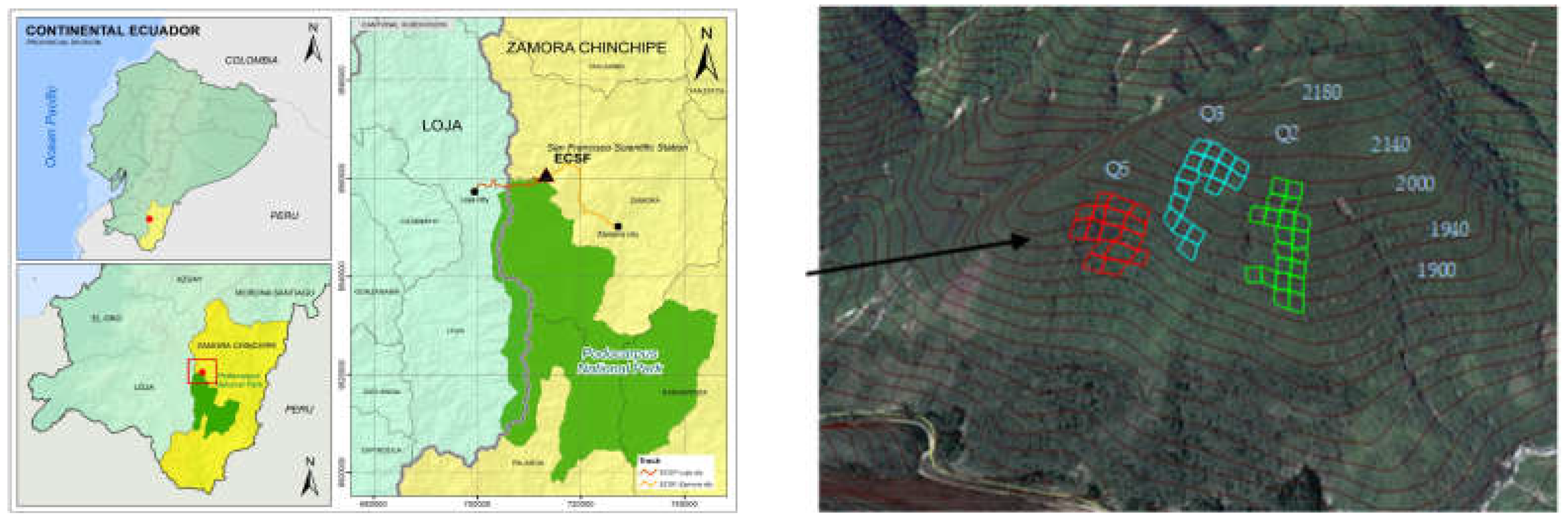
2.1. General Description of the Study Site
2.2. Installation of Plots and Forest Inventory
2.3. Data Acquisition
2.4. Data Analyses
2.5. Statistic Analysis
2.5.1. Non-Metric Multidimensional Scaling (NMDS)
2.5.2. Canonical Correspondence Analyses
2.5.3. Correlation
2.5.4. Fourth Corner
3. Results
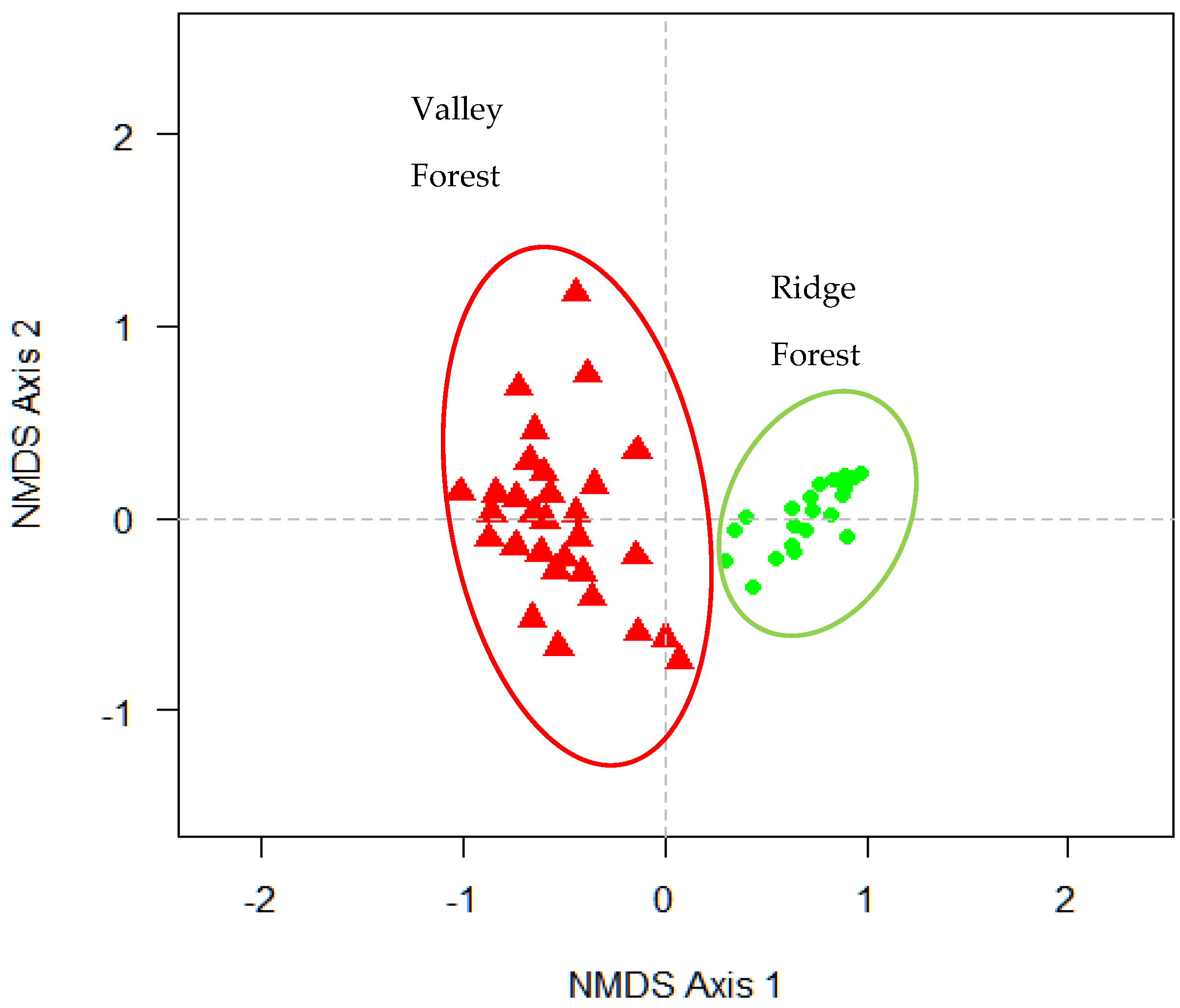
3.1. Grouping Plots
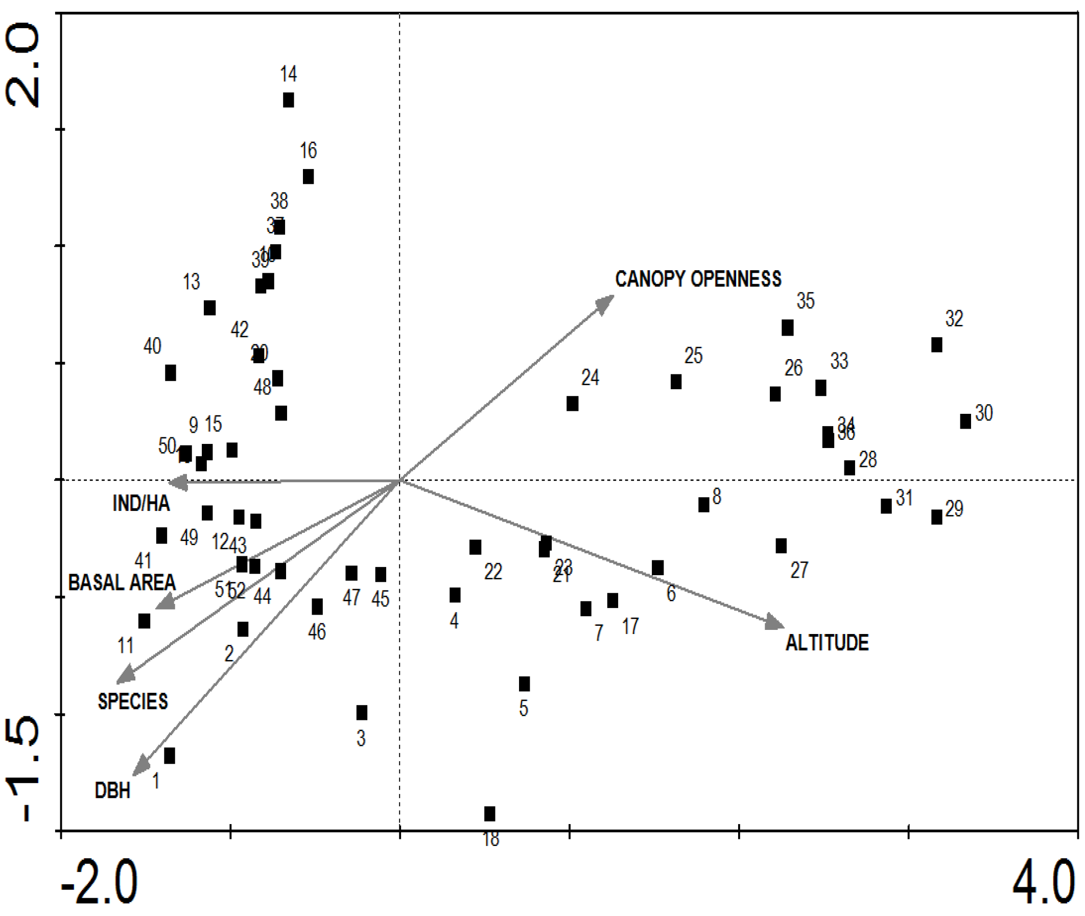
3.2. Influence of Altitudinal and Structural Parameters on Grouping Communities
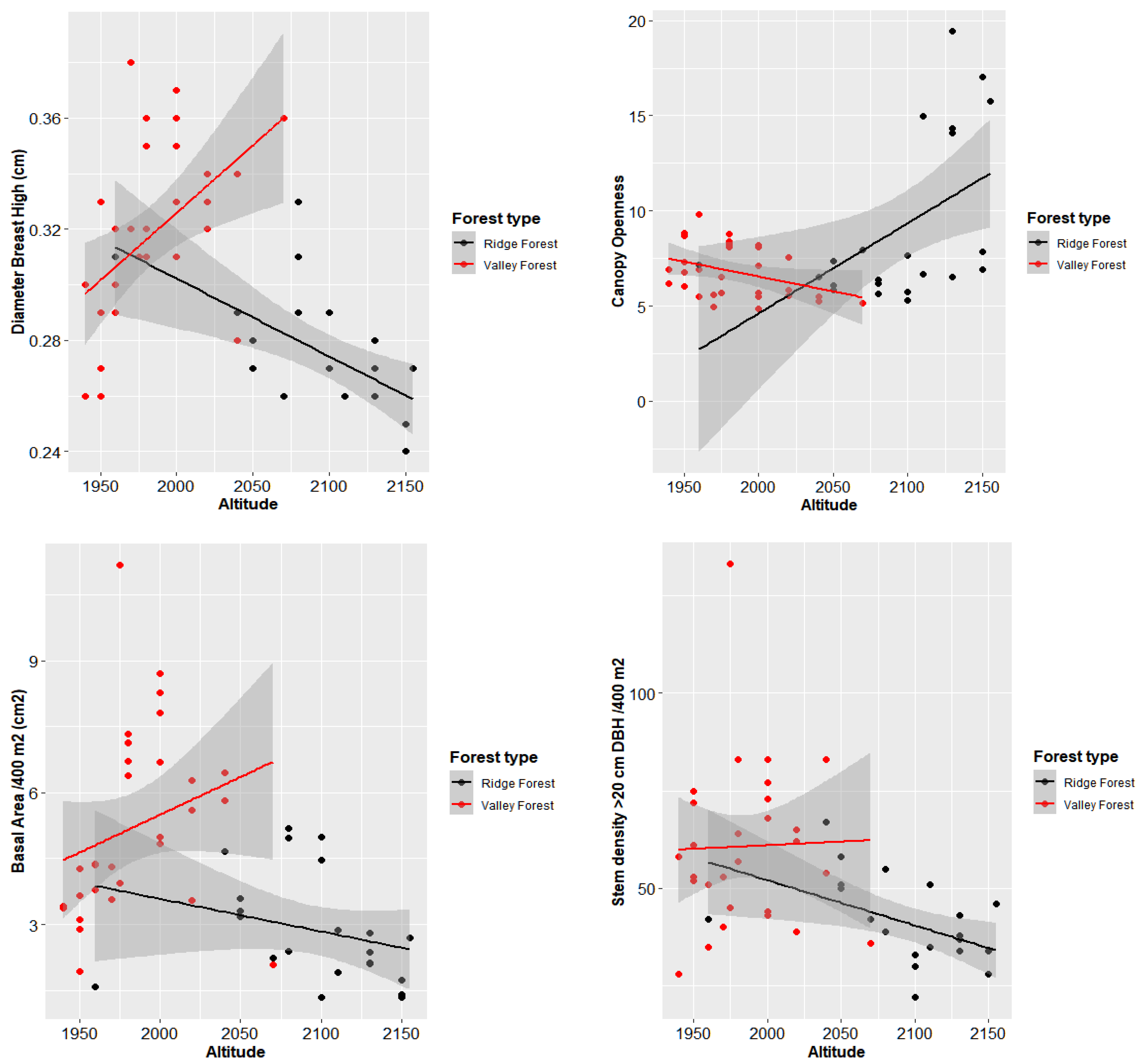
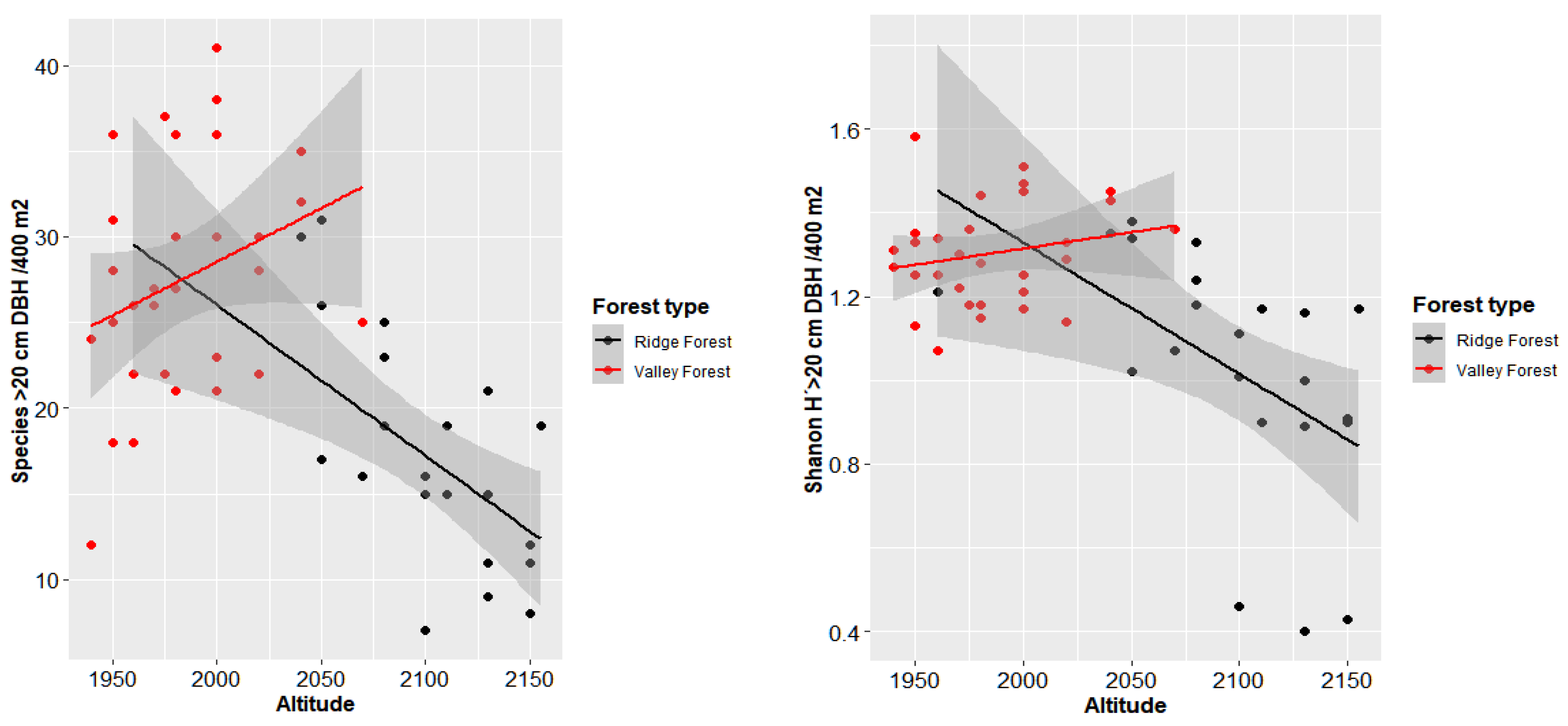
3.3. Correlation between Elevation and Characteristic of Forest
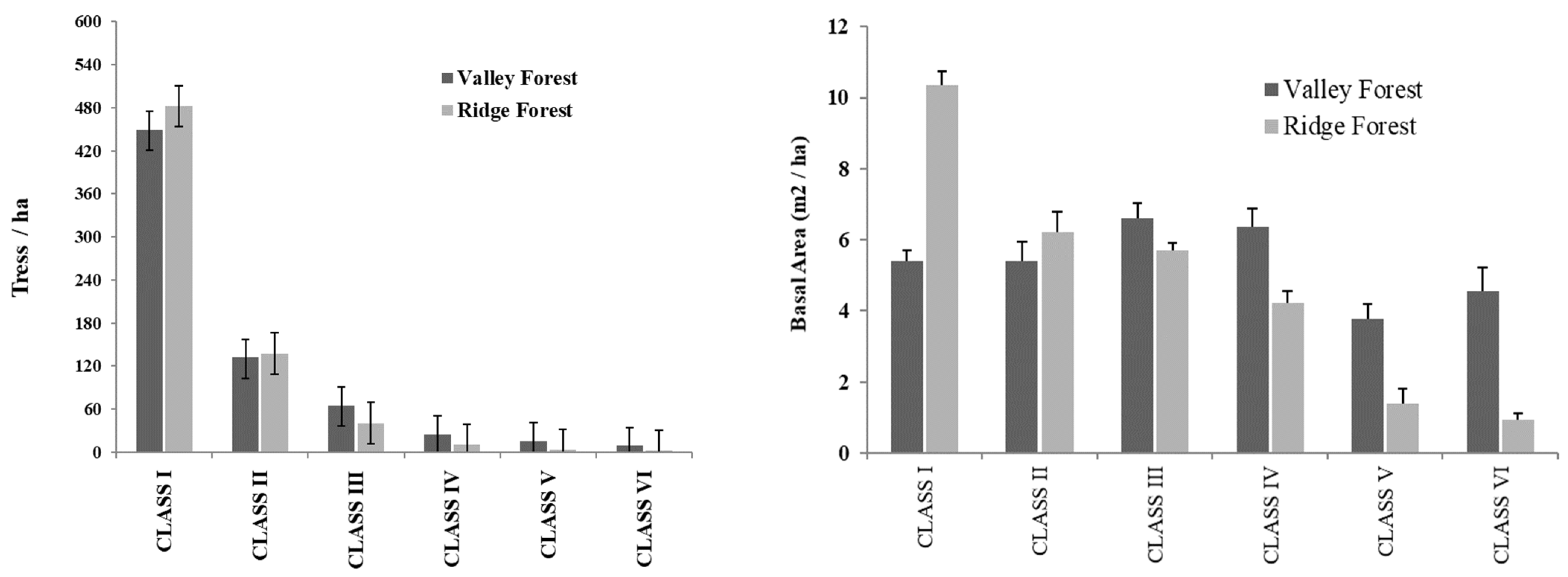
3.4. Structural Parameters of Floristic Groups
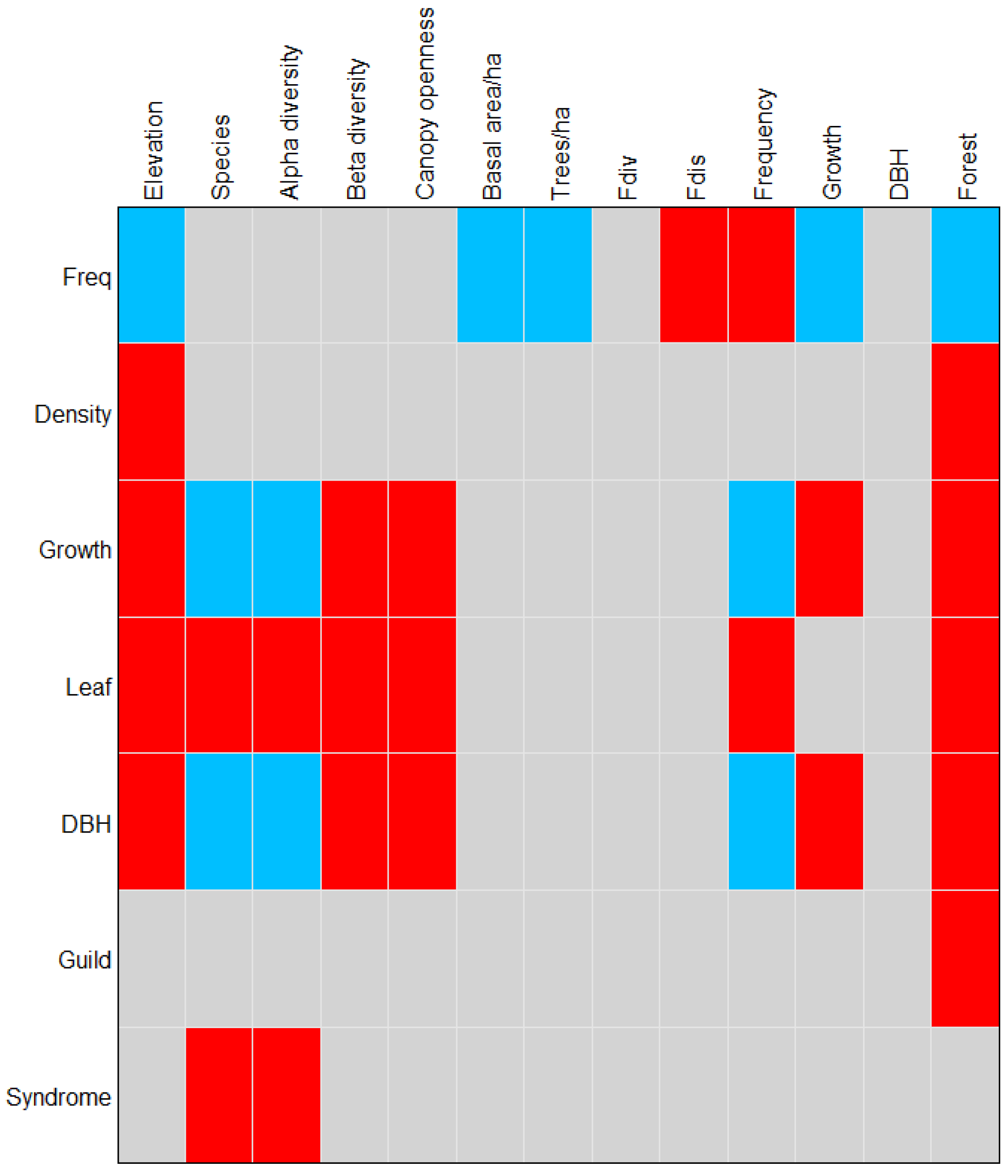
3.5. Functional Traits Influence Forest Separation
4. Discussion
Author Contributions
Funding
Institutional Review Board Statement
Informed Consent Statement
Data Availability Statement
Acknowledgments
Conflicts of Interest
References
- Saatchi, S.S.; Harris, N.L.; Brown, S.; Lefsky, M.; Mitchard, E.T.; Salas, W.; Zutta, B.R.; Buermann, W.; Lewis, S.L.; Hagen, S. Benchmark. Map of forest carbon stocks in tropical regions across three continents. Proc. Natl. Acad. Sci. USA 2011, 108, 9899–9904. [Google Scholar] [CrossRef] [PubMed]
- Myers, N.; Mittermeier, R.A.; Mittermeier, C.G.; Da Fonseca, G.A.; Kent, J. Biodiversity hotspots for conservation priorities. Nature 2000, 403, 853–858. [Google Scholar] [CrossRef] [PubMed]
- Kier, G.; Mutke, J.; Dinerstein, E.; Ricketts, T.H.; Küper, W.; Kreft, H.; Barthlott, W. Global patterns of plant diversity and floristic knowledge. J. Biogeogr. 2005, 32, 1107–1116. [Google Scholar] [CrossRef]
- Pan, Y.; Birdsey, R.A.; Fang, J.; Houghton, R.; Kauppi, P.E.; Kurz, W.A.; Phillips, O.; Shvidenko, A.; Lewis, S.L.; Canadell, J.G.; et al. A large and persistent carbon sink in the world’s forests. Science 2011, 333, 988–993. [Google Scholar] [CrossRef]
- Malhi, Y.; Phillips, O.L. Tropical forests and global atmospheric change: A synthesis. Philos. Trans. R. Soc. B 2004, 359, 549–555. [Google Scholar] [CrossRef]
- FAO. Global Forest Resources Assessment 2005. Main Repor. Progress Towards Sustainable Forest Management; FAO Forestry Papers, FAO: Rome, Italy, 2006; p. 147. [Google Scholar]
- Cirimwami, L.; Doumenge, C.; Kahindo, J.M.; Amani, C. The effect of elevation on species richness in tropical forests depends on the considered lifeform: Results from an East African mountain forest. Trop. Ecol. 2019, 60, 473–484. [Google Scholar] [CrossRef]
- Homeier, J.; Breckle, S.W.; Günter, S.; Rollenbeck, R.T.; Leuschner, C. Tree Diversity, Forest Structure and Productivity along Altitudinal and Topographical Gradients in a Species-Rich Ecuadorian Montane Rain Forest. Biotropica 2010, 42, 140–148. [Google Scholar] [CrossRef]
- Apaza-Quevedo, A.; Lippok, D.; Hensen, I.; Schleuning, M.; Both, S. Elevation, topography, and edge effects drive functional composition of woody plant species in tropical montane forests. Biotropica 2015, 47, 449–458. [Google Scholar] [CrossRef]
- Valencia, R.; Churchill, S.P.; Balslev, H.; Forero, E.; Luteyn, J.L. Composition and structure of an Andean Forest fragment in eastern Ecuador. In Biodiversity and Conservation of Neotropical Montane Forests. Proceedings of a Symposium, New York Botanical Garden; New York Botanical Garden: New York, NY, USA, 1995. [Google Scholar]
- Mosandl, R.; Günter, S.; Stimm, B.; Weber, M. Ecuador suffers the highest deforestation rate in South America. In Gradients in a Tropical Mountain Ecosystem of Ecuador; Springer: Berlin/Heidelberg, Germany, 2008. [Google Scholar]
- Valencia, R.; Cerón, C.; Palacios, W. Las formaciones naturales de la Sierra del Ecuador. In Propuesta Preliminar de un Sistema de Clasificación de Vegetación Para el Ecuador Continental; Sierra, R., Ed.; Proyecto INEFAN/GEF-BIRF and EcoCiencia: Quito, Ecuador, 1999; pp. 81–108. [Google Scholar]
- Balslev, H.; Øllgaard, B. Mapa de vegetación del sur de Ecuador. In Botánica Austroecuatoriana; Ediciones Abya-Yala: Quito, Ecuador, 2002; pp. 51–64. [Google Scholar]
- Sierra, R. Propuesta Preliminar de un Sistema de Clasificación de Vegetación Para el Ecuador Continental; Proyecto Inefan/Gef-Birf y Ecociencia: Quito, Ecuador, 1999. [Google Scholar]
- Ohl, C.; Bussmann, R. Recolonisation of natural landslides in tropical mountain forests of Southern Ecuador. Feddes Repert. 2004, 115, 248–264. [Google Scholar] [CrossRef]
- Brehm, G.; Homeier, J.; Fiedler, K. Beta diversity of geometrid moths (Lepidoptera: Geometridae) in an Andean montane rainforest. Divers. Distrib. 2003, 9, 351–366. [Google Scholar] [CrossRef]
- Schrumpf, M.; Guggenberger, G.; Valarezo, C.; Zech, W. Tropical montane rain forest soils. Development and nutrient status along an altitudinal gradient in the south Ecuadorian Andes. Erde 2001, 132, 43–59. [Google Scholar]
- Wilcke, W.; Yasin, S.; Schmitt, A.; Valarezo, C.; Zech, W. Soils along the altitudinal transect and in catchments. In Gradients in a Tropical Mountain Ecosystem of Ecuador; Springer: Berlin/Heidelberg, Germany, 2008; pp. 75–85. [Google Scholar]
- Fries, A.; Rollenbeck, R.; Bayer, F.; Gonzalez, V.; Oñate-Valivieso, F.; Peters, T.; Bendix, J. Catchment precipitation processes in the San Francisco valley in southern Ecuador: Combined approach using high-resolution radar images and in situ observations. Meteorol. Atmos. Phys 2014, 126, 13–29. [Google Scholar] [CrossRef]
- Zanne, A.E.; Lopez-Gonzalez, G.; Coomes, D.A.; Ilic, J.; Jansen, S.; Lewis, S.L.; Chave, J. Global Wood Density Database. Dryad. Identifier. 2009. Available online: http://datadryad.org/handle/10255/dryad.235 (accessed on 23 January 2023).
- Chave, J.; Coomes, D.A.; Jansen, S.; Lewis, S.L.; Swenson, N.G.; Zanne, A.E. Towards a worldwide wood economics spectrum. Ecol. Lett. 2009, 12, 351–366. [Google Scholar] [CrossRef]
- MAE. Resultados de la Evaluación Nacional Forestal; Ministerio del Ambiente: Quito, Ecuador, 2014. [Google Scholar]
- Palacios, W.A. Forest species communities in tropical rain forest of Ecuador. Lyonia 2004, 7, 33–40. [Google Scholar]
- Osazuwa-Peters, O.L.; Jiménez, I.; Oberle, B.; Chapman, C.A.; Zanne, A.E. Selective logging: Do rates of forest turnover in stems, species composition and functional traits decrease with time since disturbance? A 45 year perspective. For. Ecol. Manag 2015, 357, 10–21. [Google Scholar] [CrossRef]
- Dos Santos, V.A.H.F.; Ferreira, M.J. Are photosynthetic leaf traits related to the first-year growth of tropical tree seedlings? A light-induced plasticity test in a secondary forest enrichment planting. For. Ecol. Manag 2020, 460, 117900. [Google Scholar] [CrossRef]
- Wang, C.; Zhou, J.; Xiao, H.; Liu, J.; Wang, L. Variations in leaf functional traits among plant species grouped by growth and leaf types in Zhenjiang, China. J. For. Res. 2017, 28, 241–248. [Google Scholar] [CrossRef]
- Jara-Guerrero, A.; De la Cruz, M.; Méndez, M. Seed dispersal spectrum of woody species in south Ecuadorian dry forests: Environmental correlates and the effect of considering species abundance. Biotropica 2011, 43, 722–730. [Google Scholar] [CrossRef]
- Aguirre Calderón, Ó.A.; Jiménez Pérez, J.; Kramer, H.; Akça, A. Análisis estructural de ecosistemas forestales en el Cerro del Potosí, Nuevo León, México. Ciencia 2003, 6. [Google Scholar]
- Cerón, C. Manual de Botánica Ecuatoriana, Sistemática y Métodos de Estudio, Escuela de Biología; Universidad Central del Ecuador: Quito, Ecuador, 1993. [Google Scholar]
- Madsen, J.E.; Øllgaard, B. Floristic composition, structure, and dynamics of an upper montane rain forest in Southern Ecuador. Nord. J. Bot. 1994, 14, 403–423. [Google Scholar] [CrossRef]
- Madsen, J.E. Floristic Composition, Structure and Dynamics of an Upper Montane Rain Forest in Southern Ecuador. Ph.D. Thesis, Botanical Institute of Aarhus University, Aarhus, Denmark, 1991. [Google Scholar]
- Finol, U.H.; Finol, U.H. Estudio fitosociológico de las unidades 2 y 3 de la Reserva Forestal de Caparo, Estado Barinas. Acta Botánica Venez. 1976, 11, 15–103. [Google Scholar]
- Galindo, R.; Betancur, J.; Cadena, J.J. Estructura y composición florística de cuatro bosques andinos del santuario de flora y fauna Guanentá-Alto río Fonce, cordillera oriental colombiana. Caldasia 2003, 25, 313–335. [Google Scholar]
- Mori, S.A.; Boom, B.M.; de Carvalino, A.M. Ecological importance of Myrtaceae in an eastern Brazilian wet forest. Biotropica 1983, 15, 68–70. [Google Scholar] [CrossRef]
- Magurran, A.E. Why diversity? In Ecological Diversity and Its Measurement; Springer: Dordrecht, The Netherlands, 1988; pp. 1–5. [Google Scholar]
- Petchey, O.L.; Gaston, K.J. Functional diversity: Back to basics and looking forward. Ecol. Lett. 2006, 9, 741–758. [Google Scholar] [CrossRef]
- Cayuela, L. Una Introduccion a R. EcoLab, Centro Andaluz de Medio Ambiente; Universidad de Granada: Granada, Spain, 2010; 109p. [Google Scholar]
- Legendre, P.; Galzin, R.; Harmelin-Vivien, M.L. Relating behavior to habitat: Solutions to the fourth-corner problem. Ecology 1997, 78, 547–562. [Google Scholar] [CrossRef]
- Dray, S.; Choler, P.; Dolédec, S.; Peres-Neto, P.R.; Thuiller, W.; Pavoine, S.; ter Braak, C.J. Combining the fourth-corner and the RLQ methods for assessing trait responses to environmental variation. Ecology 2014, 95, 14–21. [Google Scholar] [CrossRef]
- Dray, S.; Legendre, P. Testing the species traits–environment relationships: The fourth-corner problem revisited. Ecology 2008, 89, 3400–3412. [Google Scholar] [CrossRef]
- Aubin, I.; Ouellette, M.H.; Legendre, P.; Messier, C.; Bouchard, A. Comparison of two plant functional approaches to evaluate natural restoration along an old-field–deciduous forest chronosequence. J. Veget. Sci. 2009, 20, 185–198. [Google Scholar] [CrossRef]
- Chessel, D.; Dufour, A.B.; Dray, S. Analysis of Ecological Data: Exploratory and Euclidean Methods in Environmental Sciences. Version 1.4-14. 2 October 2010; Lyon, France1: 4, 11. 2009. Available online: http://pbil.univ-lyon1.fr/ADE-4/ade4-html/00Index.html (accessed on 23 January 2023).
- Homeier, J.; Leuschner, C.; Bräuning, A.; Cumbicus, N.L.; Hertel, D.; Martinson, G.O.; Spannl, S.; Veldkamp, E. Effects of nutrient addition on the productivity of montane forests and implications for the carbon cycle. In Ecosystem Services, Biodiversity and Environmental Change in a Tropical Mountain Ecosystem of South Ecuador; Springer: Berlin/Heidelberg, Germany, 2013; pp. 315–329. [Google Scholar]
- Werner, F.A.; Homeier, J. Is tropical montane forest heterogeneity promoted by a resource-driven feedback cycle? Evidence from nutrient relations, herbivory and litter decomposition along a topographical gradient. Funct. Ecol. 2015, 29, 430–440. [Google Scholar] [CrossRef]
- Paulick, S.; Dislich, C.; Homeier, J.; Fischer, R.; Huth, A. The carbon fluxes in different successional stages: Modelling the dynamics of tropical montane forests in South Ecuador. For. Ecosyst. 2017, 4, 5. [Google Scholar] [CrossRef]
- Paulsch, A. Development and Application of a Classification System for Undisturbed and Disturbed Tropical Montane Forests Based on Vegetation Structure. Ph.D. Dissertation, Fakultat fur Biologie, Chemie und Geowissenschaften der Universitat Bayreuth, Bayreuth, Germany, 2002. [Google Scholar]
- Homeier, J. Baumdiversität, Waldstruktur und Wachstumsdynamik Zweier-Tropischer Bergregenwälder in Ecuador und Costa Rica. Ph.D. Thesis, University of Bielefeld, Bielefeld, Germany, 2004. [Google Scholar]
- Parolly, G.; Kürschner, H. Ecosociological studies in Ecuadorian bryophyte communities. V. Syntaxonomy, life forms and life strategies of the bryophyte vegetation on decaying wood and tree bases in S Ecuador. Nova Hedwigia 2005, 81, 1–36. [Google Scholar] [CrossRef]
- Homeier, J.; Werner, F.A.; Gradstein, S.R.; Breckle, S.; Richter, M. Potential vegetation and floristic composition of Andean forests in South Ecuador, with a focus on the RBSF. Ecol. Stud. 2008, 198, 87. [Google Scholar]
- Kuebler, D.; Hildebrandt, P.; Günter, S.; Stimm, B.; Weber, M.; Mosandl, R.; Muñoz, J.; Cabrera, O.; Aguirre, N.; Zeilinger, J.; et al. Assessing the importance of topographic variables for the spatial distribution of tree species in a tropical mountain forest. Erdkunde 2016, 70, 19–47. [Google Scholar] [CrossRef]
- Liu, J.; Yunhong, T.; Slik, J.F. Topography related habitat associations of tree species traits, composition and diversity in a Chinese tropical forest. For. Ecol. Manag. 2014, 330, 75–81. [Google Scholar] [CrossRef]
- Duivenvoorden, J.F.; Cuello, A.N. Functional trait state diversity of A ndean forests in Venezuela changes with altitude. J. Veg. Sci. 2012, 23, 1105–1113. [Google Scholar] [CrossRef]
- Malhado, A.C.M.; Malhi, Y.; Whittaker, R.J.; Ladle, R.J.; ter Steege, H.; Phillips, O.L.; Butt, N.; Aragão, L.E.O.C.; Quesada, C.A.; Araujo-Murakami, A.; et al. Spatial trends in leaf size of Amazonian rainforest trees. Biogeosciences 2009, 6, 1563–1576. [Google Scholar] [CrossRef]
- Antonio Vazquez, G.J.; Givnish, T.J. Altitudinal gradients in tropical forest composition, structure, and diversity in the Sierra de Manantlán. J. Ecol. 1998, 86, 999–1020. [Google Scholar]
- Chave, J.; Muller-Landau, H.C.; Baker, T.R.; Easdale, T.A.; Steege, H.T.; Webb, C.O. Regional and phylogenetic variation of wood density across 2456 neotropical tree species. Ecol App. 2006, 16, 2356–2367. [Google Scholar] [CrossRef]
- Körner, C.; Paulsen, J. A world‐wide study of high altitude treeline temperatures. J. Biogeogr. 2004, 31, 713–732. [Google Scholar]
- Jadán, O.; Donoso, D.A.; Cedillo, H.; Bermúdez, F.; Cabrera, O. Floristic groups, and changes in diversity and structure of trees, in tropical montane forests in the Southern Andes of Ecuador. Diversity 2021, 13, 400. [Google Scholar]
- Treiber, J.; von Wehrden, H.; Zimmermann, H.; Welk, E.; Jäger, E.J.; Ronnenberg, K.; Wesche, K. Linking large-scale and small-scale distribution patterns of steppe plant species—An example using fourth-corner analysis. Flora 2020, 263, 151553. [Google Scholar] [CrossRef]
- Malizia, A.; Blundo, C.; Carilla, J.; Acosta, O.O.; Cuesta, F.; Duque, A.; Aguirre, N.; Aguirre, Z.; Ataroff, M.; Baez, S.; et al. Elevation and latitude drive structure and tree species composition in Andean forests: Results from a large-scale plot network. PLoS ONE 2020, 15, e0231553. [Google Scholar] [CrossRef] [PubMed]
- Moser, G.; Leuschner, C.; Hertel, D.; Graefe, S.; Soethe, N.; Iost, S. Elevation effects on the carbon budget of tropical mountain forests (S Ecuador): The role of the belowground compartment. Glob. Chang. Biol. 2011, 17, 2211–2226. [Google Scholar] [CrossRef]
- Dislich, C.; Huth, A. Modelling the impact of shallow landslides on forest structure in tropical montane forests. Ecol. Model 2012, 239, 40–53. [Google Scholar] [CrossRef]
- Bussmann, R.W. Los bosques montanos de la Reserva Biológica San Francisco (Zamora-Chinchipe, Ecuador)—Zonación de la vegetación y regeneración natural. Lyonia 2003, 3, 57–72. [Google Scholar]


| Type of Trait | Functional Trait | Categories | Unit |
|---|---|---|---|
| Acquisitive | Wood density | - | g cm3 |
| Stem density | - | number | |
| Diametric growth | - | cm year−1 | |
| Leaf type | Simple | ||
| Compound | |||
| Conservative | Ecological guild | Shade tolerant | |
| Partial shade tolerant | |||
| Partial light tolerant | |||
| Light tolerant | |||
| Anemochory | |||
| Dispersal syndrome | Zoochory | ||
| Barochory |
| Variable | Var.N | LambdaA | p | F-Ratio |
|---|---|---|---|---|
| Altitude | 4 | 0.61 | 0.001 ** | 7.09 |
| DBH | 7 | 0.24 | 0.001 ** | 3.01 |
| Species | 3 | 0.15 | 0.001 ** | 1.76 |
| Trees/ha | 2 | 0.14 | 0.030 * | 1.75 |
| Canopy Openness | 8 | 0.11 | 0.044 * | 1.38 |
| Basal Area/ha | 1 | 0.08 | 0.279 | 1.09 |
| Valley Forest | Ridge Forest | ||||
|---|---|---|---|---|---|
| FAMILIES | Species | Relative Diversity (%) | FAMILIES | # Species | Relative Diversity (%) |
| Lauraceae | 17 | 12.06 | Lauraceae | 23 | 27.7 |
| Moraceae | 13 | 9.22 | Euphorbiaceae | 7 | 8.4 |
| Euphorbiaceae | 10 | 7.09 | Rubiaceae | 5 | 6 |
| Melastomataceae | 9 | 6.38 | Melastomataceae | 4 | 4.8 |
| Meliaceae | 9 | 6.38 | Myrtaceae | 4 | 4.8 |
| Cecropiaceae | 4 | 2.84 | Clusiaceae | 3 | 3.6 |
| Mimosaceae | 4 | 2.84 | Cunnoniaceae | 3 | 3.6 |
| Myrtaceae | 4 | 2.84 | Aquifoliaceae | 2 | 2.4 |
| Aquifoliaceae | 2 | 2.13 | Arecaceae | 2 | 2.4 |
| Other families (41) | 1–2 | 0.71–2.13 | Asteraceae | 2 | 2.4 |
| Meliaceae | 2 | 2.4 | |||
| Mimosaceae | 2 | 2.4 | |||
| Moraceae | 2 | 2.4 | |||
| Myrsinaceae | 2 | 2.4 | |||
| Sapindaceae | 2 | 2.4 | |||
| Sapotaceae | 2 | 2.4 | |||
| Other families (16) | 1 | 1.2 | |||
| Valley Forest | ||
|---|---|---|
| Species | Relative Density (%) | Relative Dominance (%) |
| Cecropia montana | 10.52 | 15.04 |
| Tabebuia chrysantha | 4.82 | 13.53 |
| Guarea pterorhachis | 4.46 | 10.54 |
| Cecropia gabrielis | 4.15 | 5.58 |
| Heliocarpus americanus | 3.63 | 6.13 |
| Hyeronima asperifolia | 3.42 | 7.54 |
| Piptocoma discolor | 6.63 | |
| Tapirira obtuse | 5.57 | |
| Sapium glandulosum | 3.27 | 4.58 |
| Miconia quadripora | 3.11 | 4.61 |
| Inga acreana | 2.64 | |
| Nectandra membranacea | 2.54 | |
| Other species | 0.5–2.64 | 0.05–3.57 |
| Ridge Forest | ||
|---|---|---|
| Species | Relative Density (%) | Relative Dominance (%) |
| Alchornea grandiflora | 11.95 | 13.37 |
| Alzatea verticillata | 10.67 | 15.03 |
| Clusia ducoides | 10.44 | 10.06 |
| Graffenrieda emarginata | 7.77 | 5.37 |
| Purdiaea nutans | 5.57 | 5.45 |
| Hyeronima moritziana | 3.83 | 3.52 |
| Podocarpus oleifolius | 3.71 | 4.23 |
| Tapirira obtusa | 3.36 | 3.86 |
| Myrcia sp. | 3.25 | 2.35 |
| Dictyocaryum lamarckianum | 2.67 | |
| Naucleopsis glabra | 2.2 | |
| Persea ferruginea | 1.86 | |
| Alchornea pearcei | 1.74 | 2.65 |
| Clusia elliptica | 1.74 | |
| Nectandra sp. | 1.74 | |
| Vismia tomentosa | 1.62 | |
| Persea sp. | 1.51 | |
| Myrsine coriácea | 1.39 | |
| Hyeronima asperifolia | 1.28 | |
| Matayba inelegans | 1.16 | |
| Other species (58) | 0.93–0.12 | |
| Other species (76) | 0.06–2.27 | |
| Traits | Test | Stat. Obs | Std. Obs | Alter | p-Value | p-Value .adj | |
|---|---|---|---|---|---|---|---|
| Altitude | FREC | R | 0.103 | 3.021 | two-sided | 0.007 | 0.019 * |
| AB. HA | FREC | R | 0.127 | 3.716 | two-sided | 0.001 | 0.004 ** |
| ARB.HA | FREC | R | −0.126 | −3.713 | two-sided | 0.001 | 0.004 ** |
| Fdis | FREC | r | 0.093 | 2.609 | two-sided | 0.019 | 0.049 * |
| FREC | FREC | r | 0.156 | 4.515 | two-sided | 0.001 | 0.004 ** |
| Growth | FREC | r | −0.129 | 3.589 | two-sided | 0.003 | 0.011 * |
| Forest | FREC | r | 0.102 | 3.032 | two-sided | 0.005 | 0.016 * |
| Altitude | Density | r | 0.140 | 4.090 | two-sided | 0.002 | 0.008 ** |
| Forest | density | r | 0.115 | 3.327 | two-sided | 0.004 | 0.014 * |
| Altitude | Growth | r | 0.254 | 7.673 | two-sided | 0.001 | 0.004 ** |
| Species | Growth | r | 0.159 | 4.652 | two-sided | 0.001 | 0.004 ** |
| diver.A | Growth | r | 0.188 | 5.568 | two-sided | 0.001 | 0.004 ** |
| diver.B | growth | r | 0.185 | 5.449 | two-sided | 0.001 | 0.004** |
| CO | growth | r | 0.136 | 4.073 | two-sided | 0.001 | 0.004 ** |
| FREC | Growth | r | 0.142 | 4.132 | two-sided | 0.002 | 0.008 ** |
| Forest | Growth | r | 0.238 | 7.201 | wo-sided | 0.001 | 0.004 ** |
| Altitude | LEAF | F | 5.027 | 9.009 | Greater | 0.001 | 0.004 ** |
| Species | LEAF | F | 6.133 | 1.133 | Greater | 0.001 | 0.004 ** |
| diver.A | LEAF | F | 4.652 | 8.274 | Greater | 0.002 | 0.008 ** |
| diver.B | LEAF | F | 3.064 | 5.131 | greater | 0.007 | 0.019 * |
| CO | LEAF | F | 2.027 | 3.387 | Greater | 0.013 | 0.035 * |
| FREC | LEAF | F | 2.887 | 4.742 | Greater | 0.006 | 0.018 * |
| DBH | LEAF | F | 1.821 | 3.053 | Greater | 0.022 | 0.05. |
| Forest | LEAF | F | 8.230 | 1.433 | Greater | 0.001 | 0.004 ** |
| altitud | DBH | r | 0.298 | 8.638 | two-sided | 0.001 | 0.004 ** |
| Species | DBH | r | 0.215 | 6.213 | two-sided | 0.001 | 0.004 ** |
| diver. A | DBH | r | 0.272 | 7.984 | two-sided | 0.001 | 0.004 ** |
| diver. B | DBH | r | 0.262 | 7.776 | two-sided | 0.001 | 0.004 ** |
| CO | DBH | r | 0.183 | 5.216 | two-sided | 0.001 | 0.004 ** |
| FREC | DBH | r | 0.117 | 3.438 | two-sided | 0.004 | 0.014 * |
| growth | DBH | r | 0.105 | 3.035 | two-sided | 0.005 | 0.016 * |
| Forest Type | DBH | r | 0.275 | 8.205 | two-sided | 0.001 | 0.004 ** |
| Altitude | GUILD | F | 8.883 | 2.810 | Greater | 0.023 | 0.05. |
| Forest | GUILD | F | 1.161 | 4.166 | greater | 0.007 | 0.019 * |
| Species | SYND | F | 21.493 | 5.452 | Greater | 0.005 | 0.016 * |
| diver. A | SYND | F | 14.803 | 3.061 | Greater | 0.016 | 0.042 * |
Disclaimer/Publisher’s Note: The statements, opinions and data contained in all publications are solely those of the individual author(s) and contributor(s) and not of MDPI and/or the editor(s). MDPI and/or the editor(s) disclaim responsibility for any injury to people or property resulting from any ideas, methods, instructions or products referred to in the content. |
© 2023 by the authors. Licensee MDPI, Basel, Switzerland. This article is an open access article distributed under the terms and conditions of the Creative Commons Attribution (CC BY) license (https://creativecommons.org/licenses/by/4.0/).
Share and Cite
Cabrera, O.; Ramón, P.; Stimm, B.; Gunter, S.; Mosandl, R. Functional Traits and Local Environmental Conditions Determine Tropical Rain Forest Types at Microscale Level in Southern Ecuador. Diversity 2023, 15, 420. https://doi.org/10.3390/d15030420
Cabrera O, Ramón P, Stimm B, Gunter S, Mosandl R. Functional Traits and Local Environmental Conditions Determine Tropical Rain Forest Types at Microscale Level in Southern Ecuador. Diversity. 2023; 15(3):420. https://doi.org/10.3390/d15030420
Chicago/Turabian StyleCabrera, Omar, Pablo Ramón, Bernd Stimm, Sven Gunter, and Reinhard Mosandl. 2023. "Functional Traits and Local Environmental Conditions Determine Tropical Rain Forest Types at Microscale Level in Southern Ecuador" Diversity 15, no. 3: 420. https://doi.org/10.3390/d15030420
APA StyleCabrera, O., Ramón, P., Stimm, B., Gunter, S., & Mosandl, R. (2023). Functional Traits and Local Environmental Conditions Determine Tropical Rain Forest Types at Microscale Level in Southern Ecuador. Diversity, 15(3), 420. https://doi.org/10.3390/d15030420