Seasonal Changes in the Size Distribution of Copepods Is Affected by Coastal Upwelling

Abstract

Water temperature controls the physiology, growth rate, distribution, and behavior of most plankton populations in the sea and thus affects the energy transfer in marine ecosystems. The present study focuses on the influence of seasonal changes in sea surface temperature on phytoplankton and the size distribution of copepods in the Arraial do Cabo Upwelling System (Brazil), where a wind-driven coastal upwelling can lead to multiple distinct bottom-up cascade effects on the food web. To address the potential effect of the seasonal changes, environmental data were obtained and the abundance of plankton determined from monthly samples collected in triplicate from 2010 to 2014. The samples were analyzed on a Benchtop FlowCAM (FC), and copepods (<1000 µm) were classified according to their Ellipses Equivalent Major Axis using image analysis software ImageJ (IJ). For IJ analysis, a batch-processing macro was built to open all FC raw images and then crop each copepod individually into a single picture. Using these images, prosome and urosome lengths were manually measured with the straight-line tool in IJ. With the combinations of measurements obtained in the IJ adjusted as FC measurements, we established a new, faster, and more effective way to measure copepods. With the copepod size classification, we found that there is a cycle in copepod size combined with the upwelling cycle that is related to temperature rather than to phytoplankton growth. Copepod abundance as a whole peaked during the autumn, winter, and spring seasons. The method performed here proved that FC is an effective tool for classifying copepod sizes and detecting seasonal variation.

1. Introduction

Zooplankton is traditionally described as a trophic link between primary producers and secondary consumers at higher trophic levels [1,2,3]. They are composed of small animals and heterotrophic protists ranging from microns up to centimeters but rarely reaching meters [4,5,6]. Due to their high diversity in shape and size, zooplanktonic organisms occupy a wide variety of ecological niches, presenting physiological and morphological plasticity [7,8,9]. Moreover, by being the trophic link between producers and consumers, they play a vital role in biogeochemical cycles and fisheries [3,10].

Different studies focus on the seasonal changes in planktonic productivity associated with the upwelling phenomenon in the Arraial do Cabo region (Brazil) that occurs intermittently throughout the year, enriching the water column with nutrients and thus providing favorable conditions for phytoplankton blooms. The microalgal bloom influences the enrichment of the pelagic trophic webs in the region, favoring the upper trophic levels [3,11]. In general, the upwelling production in the region is described according to a conceptual model based on three sequential phases: first is the upwelling phase itself, which brings cold, nutrient-rich water to the mixed layer [3,12,13]. The second is called the productive phase, when the water temperature rises coincident with an increase in the availability of dissolved nutrients, thus fueling primary production and phytoplankton biomass [14]. The last phase is the downwelling, when phytoplankton biomass decreases due to nutrient depletion and top-down control by benthic and planktonic consumers, leading to an oligotrophic and highly stratified scenario [3,11,14,15].

Nowadays, knowledge about the biological role of phytoplankton and zooplankton in the marine environment is primarily related to the size-structured food web [16]. Due to the large number of species, zooplankton occupies distinct ecological niches and plays key roles in ecosystem functioning [7], such as transferring energy to the higher trophic levels [3,7,17]. In addition, the zooplankton community is sensitive to environmental changes that have been reported in recent decades [18,19,20,21].

In the marine environment, copepods are the most abundant and diverse zooplankton group [20,22], and since several species of fish consume them, they are also responsible for most of the secondary production in the oceans [3,23]. Despite copepods being highly diverse and abundant, the size of copepods is one of the most valuable parameters revealing the ecological and physiological constraints of marine planktonic populations [9]. Many environmental conditions, like water temperature, can control physiological processes that influence the size distribution of organisms in a population, therefore changing the food availability in the marine ecosystem [9,20,24].

The size of copepods varies with the depth and temperature at which they are found [24]. Small copepods usually dominate the superficial warm waters, while large copepods can perform vertical diel migration efficiently [25]. Therefore, oceanographic phenomena, such as coastal upwelling, responsible for the mixing of water bodies, can modify the population structure of the copepod community [13,26,27].

Copepod abundance, taxonomy, and biometry are usually assessed by optical microscopy according to standard protocols [28]. Counting procedures based on abundance estimation are easier to perform because organisms do not need to be in the correct position and no specialized skill is needed, in contrast with taxonomy and biometry. Surveys that still depend on traditional microscopy to address the organism’s size as an estimate of biomass take too much time to process a sample with thousands of specimens [29]. Consequently, there is a limit to the number of samples feasible to process by traditional microscopy to allow their use in long time-series analyses of species-specific biomass. In addition, this sort of data usually depends on highly specialized professionals in taxonomy, micromanipulation, and well-preserved samples to avoid bias [29].

The broadly-used FlowCAM (Flow Cytometer and Microscopy, Fluid Imaging Tech, Inc., Yarmouth, MA, USA), which combines flow cytometry and light microscopy functionalities, was developed in the past decades as a tool for the identification, counting, and measurement of tiny planktonic organisms [30,31,32]. The process includes quantification, classification, and measurement of thousands of particles from 3 to 3000 µm, depending on the machine setup. For counting, the equipment considers the amount of sample processed (volume imaged) and the number of particles detected, which generates data about abundance. In contrast, automatic classification and measurements in FlowCAM^® are dependent on more complex features, such as a set of previously classified images and particle properties like shape and size [33]. For small spherical cells, common in the nano- and microplankton fractions, there is a significant linear relationship between volume and measurements that allows the use of FlowCAM^® to address the populational distribution of size classes and biovolumes [34]. In contrast, other micro and mesozooplanktonic organisms usually bear appendages and external structures that increase body complexity and thus reduce the efficiency of automatic measurements done by FlowCAM despite being valuable [35].

In this context, the objectives of the present study were to address the influence of seasonal and interannual changes in sea surface temperature and chlorophyll-a (Chl-a) concentration driven by upwelling on the size distribution of copepods. We hypothesize that both factors (temperature and chlorophyll-a) will be related to the size class of the copepods. We also addressed the effectiveness of automatically estimating the size and volume of copepods as provided by FlowCAM. We hypothesize that there will be a correlation between the values of the copepod volumes in FlowCAM compared to the optical microscopy measures.

2. Materials and Methods

2.1. Sampling

This study was performed at a fixed station located on the east coast of Rio de Janeiro State, Brazil (23° S 42.01° W) that has been monitored since October 1994 [3,11] (Figure 1). The work was conducted under the coordination of the Long Term Ecological Research Project “Upwelling” (PELD-RECA, http://cnpq.br/sitios-peld, accessed 28 April 2023) with data from 260 water samples and 180 plankton samples collected from January 2010 to December 2014. Sea surface temperature (°C, SST) was measured by a Horiba multiparameter probe (Model U-5000; HGS No. 7JETA790) at ~1 m depth, and from water samples taken weekly (±1 m depth) using a Nansen bottle, Chl-a concentration (mg.m⁻³) was extracted according to [36]. Both were considered proxies for shifts in ecosystem status, being upwelling <20 °C [37] that provides a bloom of phytoplankton >2.0 mg.m⁻³. In total, 260 weekly measures of STT (°C) and Chl-a concentration (mg.m⁻³) were analyzed, while zooplankton samples were analyzed only on full moon days, in the morning, because higher zooplankton biomass is found in this lunar phase. On each sampling date, three sub-surface (1 m depth, at speeds of 2 knots) horizontal hauls of three minutes each were performed in sequence, giving a total of 180 samples using a 100 μm mesh, 40 cm diameter WP2 plankton net in water about 10 m deep. Immediately after collection, samples were fixed in a 4% formalin solution diluted with seawater and previously buffered with sodium tetraborate. These samples were analyzed to estimate copepod size classes and abundance.

2.2. Sample Processing

In the laboratory, zooplankton samples were split into two parts using the Folsom Splitter [38]. One part was separated for analysis using a conventional light stereomicroscope (Zeiss Stemi SV6—Oberkochen, Germany) and the other for processing and analysis through FlowCAM^® (Falmouth, MA, USA). All samples were diluted to a final volume ranging from 200 mL to 500 mL, after which six subsamples of 1 mL were taken with a Stempel pipette, three were analyzed by conventional optical stereomicroscope (Zeiss Stemi SV6), while the three others were analyzed using the FlowCAM^® (FC) (Falmouth, MA, USA) and ImageJ (IJ) software in sequence. With the microscope, all copepods were identified to the lowest taxonomic level and measured with the help of Zeiss© Zen Image. The FC was set with a 2000 µm × 2000 µm flowcell, a 2× objective, and a D12 thick collimator. The flow rate was set to 2 mL/min in Autoimage mode with 15 frames/s. All subsamples were filtered through a 1000 µm Nytex mesh with a nominal retention equivalent of 1400 µm (hypotenuse), and the organisms were kept in suspension by using a magnetic stir plate. After filtration, the nominal retention was confirmed in three subsamples by checking that there was no copepod smaller than 1400 µm retained in the net.

Nevertheless, to increase data accuracy, all analyses were restricted to organisms with a prosome length smaller than 1000 µm (the organism size that FlowCam was able to analyze without obstructing the flow), which privileges immature (copepodites) and small species (e.g., Paracalanus quasimodo and Temora turbinata), dominant throughout the year on the coast of Arraial do Cabo [13]. The annotation of particles into the Copepoda class was done automatically by the VisualSpreadsheet© software (version 3.4.5) based on a library of previously selected images, after which a visual post-processing validation was performed. Images were captured at 2400 dpi (pixels per inch) resolution, 1024 × 768 pixels in size.

All particles were checked to eliminate misclassification. Copepod abundance (organisms.m⁻³) was estimated based on the organism counts obtained from the classification filters. The imaged volume, the initial sample volume, the subsample volume, and the net-filtered volume in each trawl were considered, expressed by the equation: Ab = {(N × VI)/VS} × (V0/VR), where Ab = copepod abundance (organisms.m⁻³), N = copepod count (organisms), VI = volume imaged (mL), VS = subsample volume (mL), V0 = initial dilution volume (mL), and VR = mesh-filtered volume (m³).

Organisms were measured at two linear distances, the length and the width of circumscribed ellipses, to address the temporal variation in the size structure of copepod assemblages over time. The prosome length was used to estimate body length in order to reduce noise in the data due to setae and appendages. This estimate was based on the ratio of the major and minor axes of the circumscribed ellipse (aspect ratio), which also considers the copepod’s position in the image. A specific algorithm in ImageJ software was developed that measures Ellipses Equivalent Major Axis (EEMA) on FlowCAM images. A significant positive correlation was found between the EEMA and the prosome length measured through microscopy (N = 100), which was then used to validate the method.

For a better understanding of Copepoda time dynamics in terms of size, eight size classes for prosome size were defined: I (≥100–<200 µm), II (≥200–<300 µm), III (≥300–<400 µm), IV (≥400–<500 µm), V (≥500–<600 µm), VI (≥600–<700 µm), VII (≥700–<800 µm), and VIII (>800 µm), after analyzing the frequency histogram of the prosome length. There is an expected overlap in prosome length between adults and immature copepodites among copepod species. Our data do not account for this difference, and all organisms were named copepods regardless of their size.

2.3. Image Processing

For IJ analysis, a batch-processing macro was built to open all FC raw images and then crop each copepod individually into a single picture. The macro, therefore, transforms all pictures into an 8-bit binary image and then removes the background by thresholding. Since the background removal process is potentially an erosion step, three threshold algorithms—Default, Otsu, and Minimum—were tested to verify which one better reduced the interference (noise) of appendages like antennae and setae on the measurement of length and biovolume. The Feret Diameter and the best-fitting ellipsis were calculated for each image. As potential proxies for prosome length [35], two measurements from IJ (the Feret Diameter and Major Axis) and three from FC (Area Based Diameter—ABD, Equivalent Spherical Diameter—ESD, and Feret Length—FL) were correlated to the actual prosome length derived from microscopy. The prosome was measured from the furthest projection of the head to the flexure joint of the urosome. The prosome width and height were measured at the widest point of the body. The urosome length was measured from the flexure joint to the insertion of the caudal setae and the width in its broadest segment. For biovolume proxies, the ellipsoid volume from IJ (calculated as 4/3 × Pi × [Minor Axis/2]² × Major Axis/2), the Area Based Volume (ABV), and Equivalent Spherical Volume (ESV) from FC were correlated to the average biovolume derived from microscopy as calculated by [39,40] and [41], in which: BV = 1/6 × π × (PL × PW2) + 1/4 × π × (UL × UW2) where BV = biovolume (μm³); PL and PW = prosome length and width (μm); UL and UW = urosome length and width (μm), respectively. The differences between prosome height and width were considered negligible. As an additional validation step, a subset of 220 images was chosen randomly to investigate performance comparison between IJ and FC in measuring the same copepod image. Since the length of an organism could not be properly estimated for specimens in frontal view (N = 48; 22%), only copepods in dorsal and lateral views (N = 172; 78%) were included in the analysis. From all remaining 172 images, prosome and urosome lengths were manually measured using ImageJ’s straight-line tool.

2.4. Data Analysis

The SST and Chl-a concentration were used as predictor variables in constructing multiple linear regression models to analyze the effects of environmental variables on Copepoda size distributions. To verify possible differences in the temporal distribution of Copepoda during upwelling and downwelling events, the parametric ANOVA test (two-way, SST, and Chl-a) was used at the 5% significance level. For this analysis, the data were transformed into log x + 1 to reach the assumptions of normality and homoscedasticity of copepod measurements. Data normality was tested by the Kolmogorov–Smirnov test, presenting a normal distribution (p > 0.05). The Levene test tested data homoscedasticity, showing homogeneity of variances (p > 0.05). The data were log-transformed to satisfy normality and homoscedasticity premises. All analyses were performed in the R package (version 3.0) [42].

The FlowCam image measurements were correlated with those from the software in ImageJ to test the validity of the FC.

3. Results

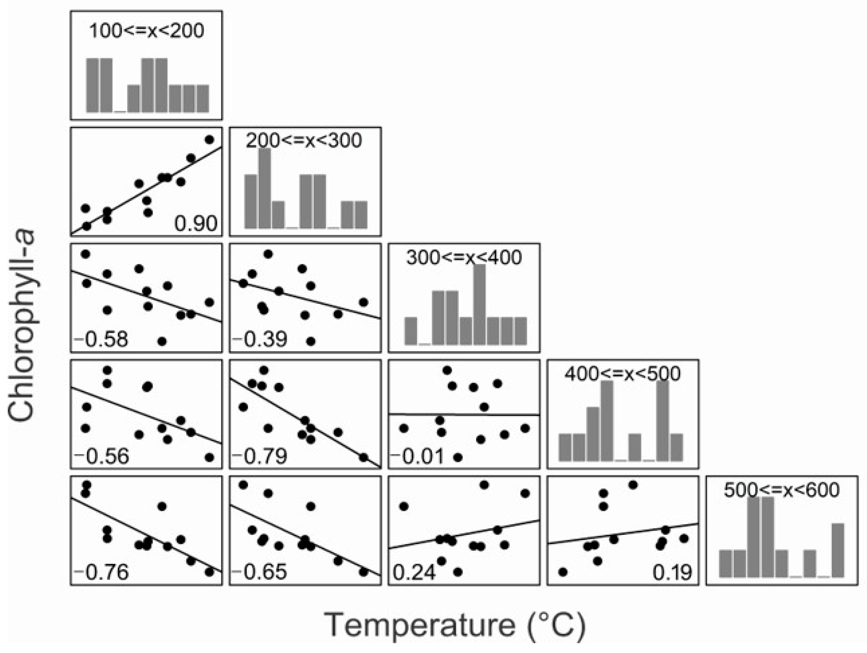
3.1. Temperature and Chlorophyll-a

The overall average sea surface temperature across the five years equals 21.6 °C ± 2.1 (S.D.) (N = 260), with a minimum of 15.2 °C and a maximum of 26.8 °C (Figure 2). In total, 19% of the time series, or nearly 50 weeks, were marked by upwelling when the average water temperature ranged from 15.2 °C to 20.0 °C (mean = 15.3 °C ± 1.3 °C SD). In contrast, downwelling periods had an average temperature of 22.4 °C, occasionally reaching a maximum of 26.8 °C. In general, sea surface temperature was highly seasonal, with warm waters in austral autumn (March–May) and cold waters in late austral winter-early spring, in all years (August–November). Apart from this seasonal trend, short-term occasional upwelling may happen in the summer, mainly in February (Figure 2). From 2010 to 2014, there was a general decreasing trend in the annual average temperature from 22.9 °C in 2010 to 20.6 °C in 2014 (linear slope = −0.53 °C year⁻¹).

Over the whole time series, the Chl-a concentration averaged 0.89 mg.m⁻³ ± 0.91 (N = 260), with a minimum under the limit of detection (~0.01 mg.m⁻³) and a maximum of 6.52 mg.m⁻³ observed in a particular week of December 2011 (Figure 2). However, 2012 showed a clearer seasonal signal, with peaks in the spring. Occasionally, a small increase in Chl-a concentration may happen during the summer (December of 2011 and January of 2012 and 2013) (Figure 2).

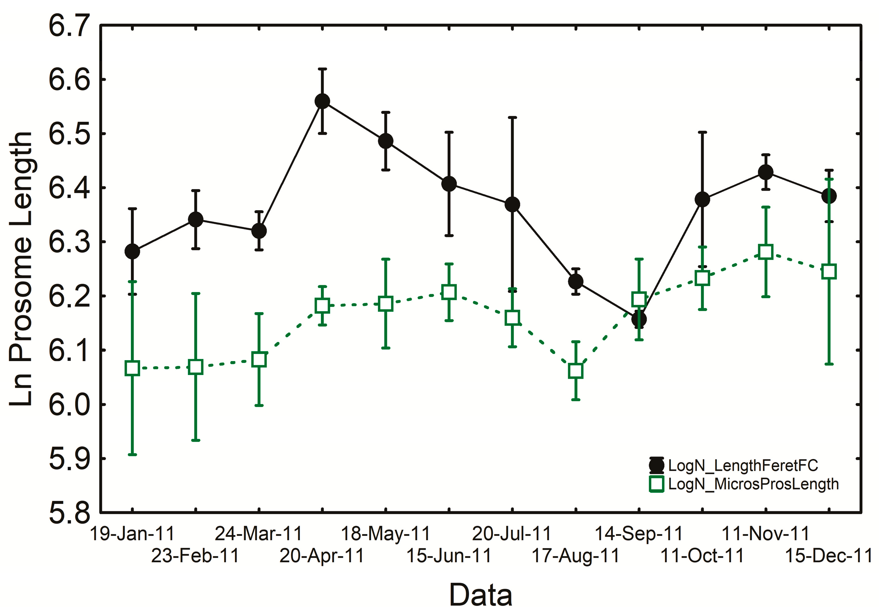
3.2. Copepod Measurements in ImageJ (IJ) and FlowCAM (FC)

There was a clear relationship between the prosomes measured by the IJ and the total length measured by the FC (R² = 0.96). Altogether, 76,671 copepod images were counted by FC and measured by both systems. IJ (prosome length) and FC (ABD area) revealed a significant (p < 0.01) positive linear correlation (R = 0.98). If we consider that the area is two-dimensional and then grows exponentially relative to the prosome length, the best fit is expressed in log10, as revealed by our data (Figure 3).

The results showed a significant (p < 0.01) positive linear correlation (R2 = 0.94) between the diameter measured by the FC and the prosome length calculated using the IJ software algorithm (Figure 4), slightly tending to underestimate the prosome length (Figure 4) when applied to a linear fit (y = ax + b). However, this tendency to underestimate the prosome length was reduced in logarithmic, whose sum of the function’s deviations (sum of squares of the deviations) is reduced from 7.2 × 107 to 3.5 × 107 and the Pearson Product-Moment Correlation Coefficient increases from 0.97 to 0.99 (Figure 4). The dominant species most measured were: Onychocorycaeus giesbrechti, Onychocorycaeus ovalis, Oncaea media, Paracalanus quasimodo, Temora stylifera, and Temora turbinata (

Table 1. Microscopy measurements (average ± S.D, μm) of copepodites, females, and males of six species of copepods. Number of individuals measured (N), prosome length (PL), prosome width (PW), urosome length (UL), total length (TL), and biovolume (BV, μm³).

Species	N	PL	PW	UL	TL	BV (106)
All grouped	1490	474 ± 121	172 ± 53	182 ± 64	656 ± 161	9.10 ± 8.06
Onychocorycaeus giesbrechti
Copepodite	19	395 ± 80	192 ± 37	199 ± 58	595 ± 130	8.59 ± 4.76
Female	11	590 ± 81	265 ± 48	338 ± 56	927 ± 76	24.13 ± 10.31
Male	31	540 ± 44	249 ± 25	350 ± 44	890 ± 45	18.70 ± 4.64
Pooled	61	504 ± 99	234 ± 44	301 ± 85	805 ± 166	16.53 ± 8.26
Onychocorycaeus ovalis
Copepodite	25	342 ± 90	180 ± 45	169 ± 68	511 ± 146	7.08 ± 5.35
Female	13	503 ± 70	261 ± 53	253 ± 44	756 ± 107	20.12 ± 11.67
Male	16	527 ± 42	243 ± 38	364 ± 70	891 ± 72	17.70 ± 6.15
Pooled	54	435 ± 113	217 ± 57	247 ± 104	682 ± 203	13.23 ± 9.45
Oncaea media
Copepodite	41	281 ± 52	105 ± 31	136 ± 31	417 ± 76	1.95 ± 1.24
Female	200	366 ± 45	146 ± 30	200 ± 38	566 ± 77	4.48 ± 1.91
Male	59	286 ± 27	111 ± 15	138 ± 23	424 ± 46	1.95 ± 0.66
Pooled	300	339 ± 58	134 ± 33	179 ± 45	517 ± 99	3.64 ± 2.04
Paracalanus quasimodo
Copepodite	128	423 ± 71	129 ± 25	127 ± 28	550 ± 94	4.15 ± 2.24
Female	506	554 ± 69	176 ± 36	174 ± 27	728 ± 90	9.82 ± 7.97
Male	112	542 ± 71	167 ± 30	173 ± 28	716 ± 95	8.66 ± 3.70
Pooled	746	530 ± 85	167 ± 38	166 ± 32	696 ± 113	8.68 ± 7.08
Temora stylifera
Copepodite	47	410 ± 147	166 ± 54	163 ± 87	573 ± 218	8.17 ± 7.54
Female	4	578 ± 65	243 ± 36	270 ± 51	848 ± 78	19.18 ± 7.48
Male	4	637 ± 25	251 ± 11	276 ± 14	913 ± 35	21.74 ± 2.78
Pooled	55	439 ± 154	178 ± 58	179 ± 90	618 ± 231	9.95 ± 8.45
Temora turbinata
Copepodite	206	437 ± 117	191 ± 62	165 ± 70	601 ± 172	10.64 ± 8.17
Female	42	595 ± 90	258 ± 48	277 ± 78	872 ± 112	22.88 ± 9.74
Male	26	617 ± 62	254 ± 37	272 ± 45	889 ± 87	22.34 ± 7.86
Pooled	274	477 ± 131	207 ± 65	192 ± 84	669 ± 198	13.59 ± 9.86

).

The abundance results revealed a significant (p < 0.01) positive (R2 = 0.45) correlation between the abundance estimated by conventional optical microscopy and FC (Figure 4), though the densities estimated by FC were one magnitude order below those expected according to microscopy. Our results revealed that the FC estimative of abundance is size-dependent based upon flow cell width (in this case, a 2000 µm flow cell), mesh size (1000 µm), and consequently group-dependent.

Out of 152 selected copepods for the algorithm test, only 119 (78%) were in lateral or dorsal position and could be used in the algorithm for validation, of which 112 (74%) exhibited the boundary between prosome and urosome needed for measurement in IJ.

The highest positive correlation (R = 0.94) was observed between the automatically estimated area of a copepod by the best-fitted ellipse and the prosome length manually measured. In general, correlations were slightly higher between automatic measurements performed by both IJ and FC and prosome length instead of copepods’ total length. By comparing both systems, correlations were lower with FC than with IJ measurements.

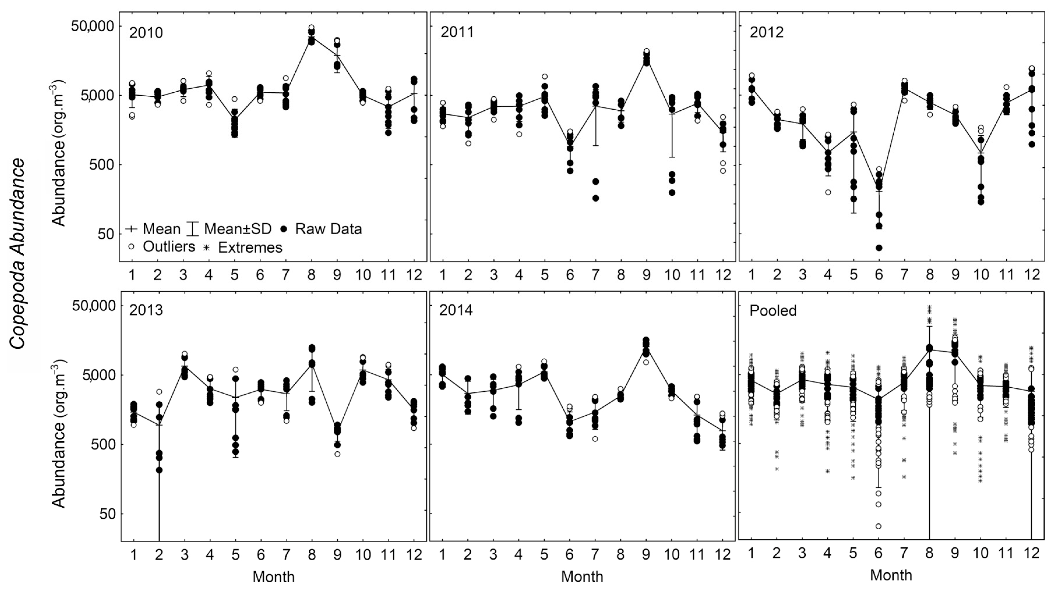
3.3. Copepod Assemblage

The copepod assemblage had an overall average of 4558 org.m⁻³ (±5618 org.m⁻³) ranging from 31 to 47,926 org.m⁻³. As expected, between year (interannual) variability was lower than within year (intra-annual) variability. The annual average was similar, with the highest annual average in 2010 (8722 ± 9596 org.m⁻³) and the lowest in 2012 (3014 ± 2639 org.m⁻³).

In general, every year is marked by one major peak in copepod abundance that occurs in late winter or early spring, between July and September (Figure 5). The peak in copepod abundance occurs one month after the seasonal increase in Chl-a.

The majority of copepods had a prosome length between 200 µm and 500 µm. The abundance of the dominant size classes (300–400 µm) had a significant relationship to temperature but not to Chl-a concentration. The abundance of small copepods was negatively correlated with temperature. During winter and spring, more than 55% of copepods were very small, with a prosome length between 100 and 300 µm. The largest copepods, with a prosome length longer than 500 µm, were more abundant during the first peak, in autumn (April and May) and in the beginning of winter (June and July), coincident with or one month after an increase in Chl-a (Figure 6).

Copepods in the first two size classes analyzed herein (100–200 µm and 200–300 µm) were positively correlated to each other (R = 0.90) through time series but negatively (up to −0.79) relative to larger ones (Figure 4). They were also negatively correlated to Chl-a concentration (R = −0.35) and sea surface temperature (R = −0.56). Despite not showing a strong correlation, the negative R-value suggests a possible inverse relationship between these two variables. In general, small copepods tend to increase in relative abundance relative to larger copepods towards the spring. In contrast, those with prosomes larger than 300 µm peak in abundance three times a year, one month after increases in Chl-a (R = 0.56) (Figure 7).

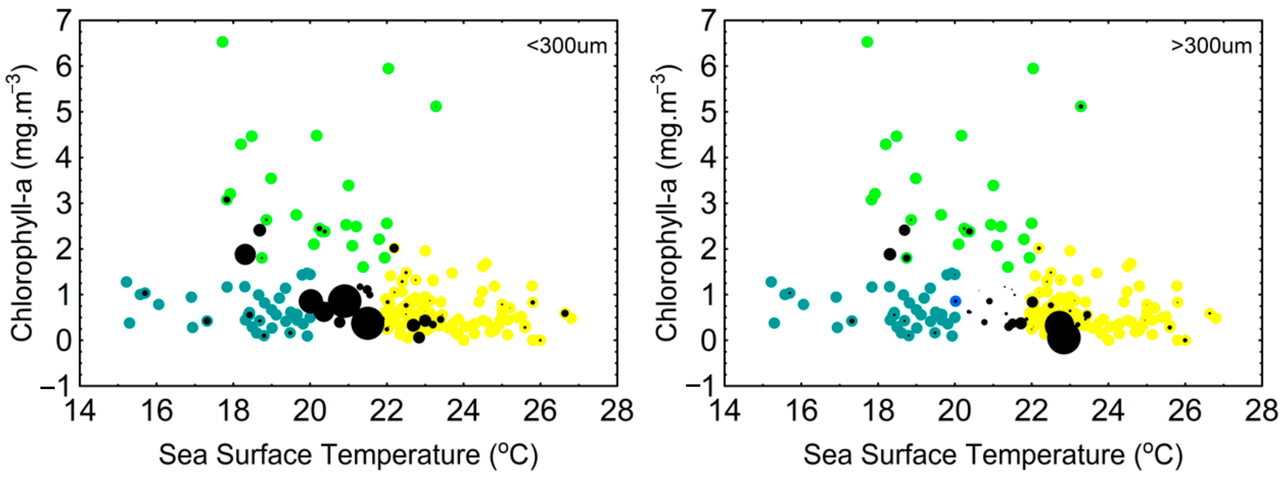
3.4. Sea Temperature Cycles’ Effect on Copepod Assemblage

Our results made it possible to describe a theoretical model of a shift in ecosystem status that occurred in the Arraial do Cabo upwelling region. The Arraial do Cabo upwelling region is an oligotrophic ecosystem most of the year, with warm water, low Chl-a concentration, and dominated by small (<300 µm prosome size) copepods (Figure 8, state 1, yellow circles). In winter and spring, upwelling brings cold (<20 °C) nutrient-rich waters into the photic zone, which turns the ecosystem into a eutrophic state (Figure 8, state 2, blue circles). As more nutrients become available and the temperature rises back up, it starts a bottom-up cascade effect that fuels phytoplankton growth and increases Chl-a concentration (Figure 8, state 3, green circles). During the next month, intense grazing by larger copepods (>300 µm) exerts a top-down control upon phytoplankton that turns Chl-a back to status 1 level. A decrease in sea temperature (down to 20 °C) drives a shift in the size structure of copepods by increasing the proportional abundance of tiny organisms (Figure 9).

4. Discussion

4.1. Temperature and Chlorophyll-a

The effects of subsidence and upwelling influence the composition and size of the copepod assemblages off the coast of Brazil and the South Atlantic. On a global scale, the temperature is one of the main factors influencing the planktonic community, and this occurs with greater intensity in regions of upwelling, as in coastal Arraial do Cabo (Brazil) [3]. The western waters of Indonesia [43] and the coast of southeast Vietnam [44] are concurrent with temperature but not as easily measured. Bi-directional trophic links (bottom-up and top-down) are thought to affect plankton communities with the same magnitude [45,46,47,48].

Our data simultaneously evaluated the relative importance of sea surface temperature and Chl-a concentration in regulating seasonal changes in copepod abundance in different size classes. The results show the effects of zooplankton size classes throughout upwelling cycles (bottom-up and top-down) on trophic links [2] and the cascading effect described on the Brazilian coast of upwelling [3]. Nevertheless, these links are species-specific and size-dependent [16].

4.2. Copepod Measurements in ImageJ (IJ) and FlowCAM (FC)

The present study showed that copepod prosoma could be represented as ellipses in software that measures particle sizes [49,50]. After converting the particles into ellipses, the area and the major and minor axes, begin to represent relevant morphometric parameters of the individuals with a certain degree of confidence [49]. Among the parameters previously mentioned, the choice of measuring the area to measure the actual particle size was made.

Data from the study reveals that the particles’ position, when processed only in the semi-automatic imaging system FC and according to [51], affects the measurement of their size in a linear measure. It is essential to point out that this position cannot be modified in retrospect because it is a photograph [52]. Nevertheless, this effect can be reduced by simultaneously estimating more than one measure of the animal [53,54].

Furthermore, the ellipse area, which is a two-dimensional measurement, showed better correlations due to less interference from the particle position [49,54]. On the other hand, depending on the particle position, the ESD diameter calculation, which is ultimately two-dimensional, overestimates the copepod’s prosome length by including cephalic appendages and the urosome [52,55] and should be changed to ABD diameter to provide a better estimative.

The advantages of using the ellipse (IJ) versus the sphere (ESD/ABD diameter—VSP) are related to the inclusion of appendages as a measure error source [56]. This inclusion does not occur when the organism is in lateral view, and the central axis becomes the best parameter for measuring the prosome length. On the other hand, when the organism is in a position other than lateral, dorsal, or ventral, for example, the minor axis is not significantly affected relative to the major, and the area becomes the best parameter to estimate the prosome length. IJ software was used to classify and measure zooplankton organisms. Other authors also concluded that the ellipse format best measures the copepods’ prosome length [49,57].

In addition to the organism’s position in the image, the absence of any body part also affects the measurement. In this study, some particles were not fully imaged since part of their bodies were cut off. The FC measured the size of these particles even though they were incomplete, generating an incorrect measurement of their actual size [35,52,58,59]. However, when processing the same particles in ImageJ software, the algorithm slightly complements the missing part of the particle by creating an ellipse around it, which acts as an adjustment to the actual particle size [60,61].

Despite problems with the copepod position (side or dorsal view), the presence of multiple organisms in the same image, and/or the absence of body parts during the classification and measurement steps, the FC is efficient in long-term analyses of copepods according to the size of the dominant species. The authors of [32] found similar results when comparing the size of phytoplankton using microscopy and FC measurements. The same conclusion seems valid for marine nano- and microplankton [62] and generalized particle size in coastal waters [63]. In contrast, our results are inconclusive for organisms larger than 1000 µm. Previous methods did not yet exist for organisms larger than 1000 µm and were only used for measurements of the flow cell boundary.

Further studies in the range 1000–2000 µm will provide new insights on the effectiveness of FC in estimating copepod abundance. Phytoplankton and generalized particles whose shapes are similar to a sphere or pear are better quantified and measured than colonial species with long chains [64]. In these cases, a new and specific algorithm for recognition and measurement will be necessary.

In the present study, the FC underestimated the copepod’s abundance by about one order of magnitude, which was clearly due to limits in size imposed by the mesh and flow cell chosen. The authors of [64] observed good correspondence when comparing the structural size of the planktonic community estimated at a fixed site simultaneously by conventional optical microscopy and FC. The authors of [65] and [31] found the same usefulness and reliability when comparing the abundance of the metazooplankton community (with a size variation between 80 and 1000 μm) and phytoplankton estimated by both conventional optical microscopy and FC. We found clear correspondence in dominant species and/or stages (copepodites), suggesting that the nauplius of copepods would be well quantified in plankton samples taken with small nets (<100 µm), but not in species larger than 1000 µm.

From investigating the factors responsible for the copepod abundance underestimation, two factors were most relevant: the exclusion of images containing multiple organisms and the size-structured planktonic community. The first issue can be solved by improving our algorithm to track such images and reprocessing them by sorting each organism. However, the second would seem to be able to be further investigated in the future since the FC system, as available now, allows processing of organisms smaller than 1000 μm [31,32].

4.3. Copepod Assemblage and Sea Temperature Cycles on Copepod Assemblage

We found opposite trends for small and large copepods (prosome cutoff = 300 µm) that can explain the apparent absence of correlation between Chl-a and the whole copepod assemblage; other authors have found the same results [66]. Occasionally in February (2013), water temperature suddenly decreased below 20 °C, suggesting a late-summer upwelling coincident with an increase in abundance of copepods (2500 org.m⁻³) but with no apparent effect on Chl-a concentration. This apparent mismatch was associated with the speedy consumption of phytoplankton by larger copepods (>300 µm) and filter-feeding organisms [11,67,68], exerting a top-down control that is not easily detectable in the monthly average.

The first peak in June or July is an austral winter bloom, and its impact on copepod abundance has at least the same intensity as the spring bloom in September. The authors of [67] were the first to highlight this increase in copepod abundance during the winter of 1992 in the Arraial do Cabo region. The authors of [13] found the same link between winter (July) rises in Chl-a and increased Paracalanus quasimodo abundance. Our results highlight this winter coupling between phytoplankton and zooplankton, but with a one month lag for small copepods.

The Calanoid copepods P. quasimodo and Temora turbinata are the most abundant species in the Arraial do Cabo region [13,14,69], feeding on a variety of items like detritus, protozoans, and phytoplankton [11,70,71]. P. quasimodo is well represented among copepod assemblages in Arraial do Cabo upwelling [13] and seems to be synchronized to the winter and spring blooms of phytoplankton.

The second peak in the second semester, in November, is the spring bloom of phytoplankton. As a bottom-up cascade effect, upwelling in September/October increases Chl-a concentration and the abundance of all-size copepods. After the spring cascade effect, an increase in Chl-a during the following summer will increase the abundance of large copepods. When [72] analyzed biological and oceanographic indicators in the Arraial do Cabo region, they also found an increase in Chl-a concentration during the summer.

Some previous studies on copepod abundance suggest that temperature strongly affects copepod abundance, metabolism, behavior, and growth [73,74,75,76]. The copepod occurrence infers seasonal changes in copepod assemblages concerning size classes. Research by [77] observed that most small copepods are omnivores feeding on autotrophic and heterotrophic organisms. A study carried out by [78] described a pattern for seasonal environments in which nearly 90% of copepod species are small species. They also suggest that Chl-a concentration is the most significant factor in body size response in juvenile copepods. In adult copepods, temperature is a more significant factor in body size response than Chl-a concentration.

According to our results, yearly changes in sea surface temperature and Chl-a concentration are not directly correlated. The expected effect of nutrient-rich cold water increasing phytoplankton biomass could not be revealed by the annual average, considering its seasonal lag. However, this correlation is highlighted when we consider the seasonal scenarios for the ecosystem state. During most of the first semester, warm waters (>20 °C) led to conspicuous stratification that in turn resulted in a low abundance of phytoplankton (<2 Chl-a.mg⁻³) and large (>300 µm) copepods as dominant. During this period, small copepods (<300 µm) represent less than 40% of the assemblage. This scenario is described herein as Ecosystem State 1 and represents most of the data. The size of copepods significantly impacts phytoplankton biomass [48,79].

5. Conclusions

The coupling between IJ software and the FC semi-automatic imaging system proved to be an effective tool in ecological monitoring of variations in copepod populations below 1000 μm. The FC semi-automatic imaging system allowed five years of collections to be processed and analyzed in a short period of time and in a complete way compared to the time used to identify, count, and measure copepods by traditional methods.

The large copepods were well correlated with changes in Chl-a concentration. In this sense, there might be effective top-down control of phytoplankton by large copepods. In contrast, small copepods were more correlated with the seasonal upwelling (spring) and the following spring bloom of phytoplankton. During the following months, an increase in grazing by both small (<300 µm) and large copepods (>300 µm) exerts an effective top-down control upon phytoplankton that turns Chl-a back to oligotrophic warm water status.

References

1. Décima, M. Zooplankton Trophic Structure and Ecosystem Productivity. Mar. Ecol. Prog. Ser. 2022, 692, 23–42. [Google Scholar] [CrossRef]
2. Everett, J.; Heneghan, R.; Blanchard, J.; Suthers, I.; Pakhomov, E.; Sykes, P.; Schoeman, D.; Baird, M.; Basedow, S.L.; Błachowiak-Samołyk, K.; et al. Self-Organisation of Zooplankton Communities Produces Similar Food Chain Lengths throughout the Ocean; In Review; Research Square LLC: Durham, NA, USA, 2022. [Google Scholar]
3. Fernandes, L.D.D.A.; Fagundes Netto, E.B.; Coutinho, R. Inter-Annual Cascade Effect on Marine Food Web: A Benthic Pathway Lagging Nutrient Supply to Pelagic Fish Stock. PLoS ONE 2017, 12, e0184512. [Google Scholar] [CrossRef]
4. Hébert, M.P.; Beisner, B.E.; Maranger, R. Linking Zooplankton Communities to Ecosystem Functioning: Toward an Effect-Trait Framework. J. Plankton Res. 2017, 39, 3–12. [Google Scholar] [CrossRef]
5. Kang, H.C.; Jeong, H.J.; Jang, S.H.; Lee, K.H. Feeding by Common Heterotrophic Protists on the Phototrophic Dinoflagellate Biecheleriopsis Adriatica (Suessiaceae) Compared to That of Other Suessioid Dinoflagellates. ALGAE 2019, 34, 127–140. [Google Scholar] [CrossRef]
6. Burki, F.; Sandin, M.M.; Jamy, M. Diversity and Ecology of Protists Revealed by Metabarcoding. Curr. Biol. 2021, 31, R1267–R1280. [Google Scholar] [CrossRef] [PubMed]
7. Chen, M.; Kim, D.; Liu, H.; Kang, C.K. Variability in Copepod Trophic Levels and Feeding Selectivity Based on Stable Isotope Analysis in Gwangyang Bay of the Southern Coast of the Korean Peninsula. Biogeosciences 2018, 15, 2055–2073. [Google Scholar] [CrossRef]
8. Dvoretsky, V.; Dvoretsky, A. Morphological Plasticity in the Small Copepod Oithona Similis in the Barents and White Seas. Mar. Ecol. Prog. Ser. 2009, 385, 165–178. [Google Scholar] [CrossRef]
9. Skjoldal, H.R. Species Composition of Three Size Fractions of Zooplankton Used in Routine Monitoring of the Barents Sea Ecosystem. J. Plankton Res. 2021, 43, 762–772. [Google Scholar] [CrossRef]
10. Fakhraee, M.; Planavsky, N.J.; Reinhard, C.T. The Role of Environmental Factors in the Long-Term Evolution of the Marine Biological Pump. Nat. Geosci. 2020, 13, 812–816. [Google Scholar] [CrossRef]
11. Fernandes, L.D.D.A.; Quintanilha, J.; Monteiro-Ribas, W.; Gonzalez-Rodriguez, E.; Coutinho, R. Seasonal and Interannual Coupling between Sea Surface Temperature, Phytoplankton and Meroplankton in the Subtropical South-Western Atlantic Ocean. J. Plankton Res. 2012, 34, 236–244. [Google Scholar] [CrossRef]
12. Oliveira, M.M.F.; Pereira, G.C.; Ebecken, N.F.F.; Oliveira, J.L.F. Multivariate Analysis of Extreme Physical, Biological and Chemical Patterns in the Dynamics of Aquatic Ecosystem. J. Environ. Prot. 2015, 6, 885–901. [Google Scholar] [CrossRef]
13. Rosa, J.C.L.; Monteiro-Ribas, W.M.; Fernandes, L.D.A. Herbivorous Copepods with Emphasis on Dynamic Paracalanus Quasimodo in an Upwelling Region. Braz. J. Oceanogr. 2016, 64, 67–74. [Google Scholar] [CrossRef]
14. Guenther, M.; Valentin, J.L. Bacterial and Phytoplankton Production in Two Coastal Systems Influenced By Distinct Eutrophication Processes. Oecologia Bras. 2008, 12, 172–178. [Google Scholar] [CrossRef]
15. Gonzalez-Rodriguez, E.; Valentin, J.L.; Andre, S.I.; Jacob, S.A. Upwelling and Downwelling at Cabo Frio (Brazil): Comparison of Biomass and Primary Production Responses. J. Plankton Res. 1992, 14, 289–306. [Google Scholar] [CrossRef]
16. Hunt, B.P.V.; Carlotti, F.; Donoso, K.; Pagano, M.; D’Ortenzio, F.; Taillandier, V.; Conan, P. Trophic Pathways of Phytoplankton Size Classes through the Zooplankton Food Web over the Spring Transition Period in the North-West Mediterranean Sea. J. Geophys. Res. Ocean. 2017, 122, 6309–6324. [Google Scholar] [CrossRef]
17. Chen, T.-C.; Ho, P.-C.; Gong, G.-C.; Tsai, A.-Y.; Hsieh, C. Finding Approaches to Exploring the Environmental Factors That Influence Copepod-Induced Trophic Cascades in the East China Sea. Diversity 2021, 13, 299. [Google Scholar] [CrossRef]
18. Moe, S.; Hobæk, A.; Persson, J.; Skjelbred, B.; Løvik, J. Shifted Dynamics of Plankton Communities in a Restored Lake: Exploring the Effects of Climate Change on Phenology through Four Decades. Clim. Res. 2022, 86, 125–143. [Google Scholar] [CrossRef]
19. Toruan, R.L.; Coggins, L.X.; Ghadouani, A. Response of Zooplankton Size Structure to Multiple Stressors in Urban Lakes. Water 2021, 13, 2305. [Google Scholar] [CrossRef]
20. Rosa, J.C.L.; Batista, L.L.; Monteiro-ribas, W.M. Tracking of Spatial Changes in the Structure of the Zooplankton Community According to Multiple Abiotic Factors along a Hypersaline Lagoon. Nauplius 2020, 28, 1–10. [Google Scholar] [CrossRef]
21. Bradford-Grieve, J.M.; Markhasena, E.L.; Rocha, C.E.F.; Abiahy, B. Copepoda. In South Atlantic Zooplankton; Boltovskoy, D., Ed.; Backhuys Publishers: Leiden, The Netherlands, 1999; pp. 869–1098. [Google Scholar]
22. Sadaiappan, B.; PrasannaKumar, C.; Nambiar, V.U.; Subramanian, M.; Gauns, M.U. Meta-Analysis Cum Machine Learning Approaches Address the Structure and Biogeochemical Potential of Marine Copepod Associated Bacteriobiomes. Sci. Rep. 2021, 11, 3312. [Google Scholar] [CrossRef]
23. Setubal, R.B.; Do Nascimento, R.A.; Bozelli, R.L. Zooplankton Secondary Production: Main Methods, Overview and Perspectives from Brazilian Studies. Int. Aquat. Res. 2020, 12, 85–99. [Google Scholar] [CrossRef]
24. Evans, L.E.; Hirst, A.G.; Kratina, P.; Beaugrand, G. Temperature-mediated Changes in Zooplankton Body Size: Large Scale Temporal and Spatial Analysis. Ecography 2020, 43, 581–590. [Google Scholar] [CrossRef]
25. Sha, Y.; Zhang, H.; Lee, M.; Björnerås, C.; Škerlep, M.; Gollnisch, R.; Herzog, S.D.; Ekelund Ugge, G.; Vinterstare, J.; Hu, N.; et al. Diel Vertical Migration of Copepods and Its Environmental Drivers in Subtropical Bahamian Blue Holes. Aquat. Ecol. 2021, 55, 1157–1169. [Google Scholar] [CrossRef]
26. Valentin, J.L. Spatial Structure of the Zooplankton Community in the Cabo Frio Region (Brazil) Influenced by Coastal Upwelling. Hydrobiologia 1984, 113, 183–199. [Google Scholar] [CrossRef]
27. Valentin, J.L.; Monteiro-Ribas, W.M.; Mureb, M.A. O Zooplâncton Das Águas Superficiais Costeiras Do Litoral Fluminense: Análise Multivariada. Ciênc. Cult. 1987, 39, 265–271. [Google Scholar]
28. Harris, R.P.; Wiebe, P.H.; Lenz, J.; Skjoldal, H.R.; Huntley, M. Zooplankton Methodology Manual; Academic Press: Cambridge, MA, USA, 2000; ISBN 0-12-327645-4. [Google Scholar]
29. Witty, L.M. Practical Guide to Identifying Freshwater Crustacean Zooplankton; Cooperative Freshwater Ecology Unit: Sudbury, ON, Canada, 2004. [Google Scholar]
30. Álvarez, E.; Moyano, M.; López-Urrutia, Á.; Nogueira, E.; Scharek, R. Routine Determination of Plankton Community Composition and Size Structure: A Comparison between FlowCAM and Light Microscopy. J. Plankton Res. 2014, 36, 170–184. [Google Scholar] [CrossRef]
31. Le Bourg, B.; Cornet-Barthaux, V.; Pagano, M.; Blanchot, J. FlowCAM as a Tool for Studying Small (80–1000 mm) Metazooplankton Communities. J. Plankton Res. 2015, 37, 666–670. [Google Scholar] [CrossRef]
32. Sieracki, C.K.; Sieracki, M.E.; Yentsch, C.S. An Imaging-in-Flow System for Automated Analysis of Marine Microplankton. Mar. Ecol. Prog. Ser. 1998, 168, 285–296. [Google Scholar] [CrossRef]
33. Álvarez, E.; López-Urrutia, Á.; Nogueira, E. Improvement of Plankton Biovolume Estimates Derived from Image-Based Automatic Sampling Devices: Application to FlowCAM. J. Plankton Res. 2012, 34, 454–469. [Google Scholar] [CrossRef]
34. Billones, R.G.; Tackx, M.L.M.; Flachier, A.T.; Zhu, L.; Daro, M.H. Image Analysis as a Tool for Measuring Particulate Matter Concentrations and Gut Content, Body Size, and Clearance Rates of Estuarine Copepods: Validation and Application. J. Mar. Syst. 1999, 22, 179–194. [Google Scholar] [CrossRef]
35. Detmer, T.M.; Broadway, K.J.; Potter, C.G.; Collins, S.F.; Parkos, J.J.; Wahl, D.H. Comparison of Microscopy to a Semi-Automated Method (FlowCAM®) for Characterization of Individual-, Population-, and Community-Level Measurements of Zooplankton. Hydrobiologia 2019, 838, 99–110. [Google Scholar] [CrossRef]
36. Lalli, C.M.; Parsons, T.R. Biological Oceanography: An Introduction; Elsevier’s Science & Technology: Oxford, UK, 1997; ISBN 0-7506-3384-0. [Google Scholar]
37. Valentin, J.L. Analyse Des Parametres Hydrobiologiques Dans La Remonte’e de Cabo Frio. Mar. Biol. 1984, 82, 259–276. [Google Scholar] [CrossRef]
38. Boltovskoy, D.C. Atlas del Zooplancton del Atlântico Sudoccidental Metodos de Trabajo Com el Zooplancton Marine; National Institute for Fisheries Research and Development: Mar del Plata, Argentina, 1981. [Google Scholar]
39. Chojnacki, J.; Hussein, M.M. Body Length and Weight of the Dominant Copepod Species in the Southern Baltic Sea. Zesz. Nauk. Akad. Roln. Szczec. 1983, 53–64. [Google Scholar]
40. Viñas, M.D.; Diovisalvi, N.R.; Cepeda, G.D. Individual Biovolume of Some Dominant Copepod Species in Coastal Waters off Buenos Aires Province, Argentine Sea. Braz. J. Oceanogr. 2010, 58, 177–181. [Google Scholar] [CrossRef]
41. Fernández Aráoz C Individual Biomass, Based on Body Measures, of Copepod Species Considered as Main Forage Items for Fishes of the Argentine Shelf. Oceanol. Acta 1991, 14, 575–580.
42. R Core Team. R: A Language and Environment for Statistical Computing; R Foundation for Statistical Computing: Vienna, Austria, 2013; Available online: http://www.r-project.org/ (accessed on 10 January 2023).
43. Supriyadi, E.; Hidayat, R. Identification of Upwelling Area of the Western Territorial Waters of Indonesia from 2000 to 2017. IJG 2020, 52, 105. [Google Scholar] [CrossRef]
44. Xiao, F.; Wu, Z.; Lyu, Y.; Zhang, Y. Abnormal Strong Upwelling off the Coast of Southeast Vietnam in the Late Summer of 2016: A Comparison with the Case in 1998. Atmosphere 2020, 11, 940. [Google Scholar] [CrossRef]
45. Cohen, J.E.; Jonsson, T.; Carpenter, S.R. Ecological Community Description Using the Food Web, Species Abundance, and Body Size. Proc. Natl. Acad. Sci. USA 2003, 100, 1781–1786. [Google Scholar] [CrossRef] [PubMed]
46. Sinistro, R. Top-down and Bottom-up Regulation of Planktonic Communities in a Warm Temperate Wetland. J. Plankton Res. 2010, 32, 209–220. [Google Scholar] [CrossRef]
47. Tiselius, P.; Belgrano, A.; Andersson, L.; Lindahl, O. Primary Productivity in a Coastal Ecosystem: A Trophic Perspective on a Long-Term Time Series. J. Plankton Res. 2016, 38, 1092–1102. [Google Scholar] [CrossRef]
48. Lynam, C.P.; Llope, M.; Möllmann, C.; Helaouët, P.; Bayliss-Brown, G.A.; Stenseth, N.C. Interaction between Top-down and Bottom-up Control in Marine Food Webs. Proc. Natl. Acad. Sci. USA 2017, 114, 1952–1957. [Google Scholar] [CrossRef] [PubMed]
49. Gorsky, G.; Ohman, M.D.; Picheral, M.; Gasparini, S.; Stemmann, L.; Romagnan, J.-B.; Cawood, A.; Pesant, S.; García-Comas, C.; Prejger, F. Digital Zooplankton Image Analysis Using the ZooScan Integrated System. J. Plankton Res. 2010, 32, 285–303. [Google Scholar] [CrossRef]
50. Herman, A.W. Design and Calibration of a New Optical Plankton Counter Capable of Sizing Small Zooplankton. Deep Sea Res. Part A Oceanogr. Res. Pap. 1992, 39, 395–415. [Google Scholar] [CrossRef]
51. Jakobsen, H.; Carstensen, J. FlowCAM: Sizing Cells and Understanding the Impact of Size Distributions on Biovolume of planktonic Community Structure. Aquat. Microb. Ecol. 2011, 65, 75–87. [Google Scholar] [CrossRef]
52. Wong, E.; Sastri, A.R.; Lin, F.S.; Hsieh, C.H. Modified FlowCAM Procedure for Quantifying Size Distribution of Zooplankton with Sample Recycling Capacity. PLoS ONE 2017, 12, e0175235. [Google Scholar] [CrossRef] [PubMed]
53. Schulze, K.; Tillich, U.M.; Dandekar, T.; Frohme, M. PlanktoVision—an Automated Analysis System for the Identification of Phytoplankton. BMC Bioinform. 2013, 14, 115. [Google Scholar] [CrossRef] [PubMed]
54. Forest, A.; Stemmann, L.; Picheral, M.; Burdorf, L.; Robert, D.; Fortier, L.; Babin, M. Size Distribution of Particles and Zooplankton across the Shelf-Basin System in Southeast Beaufort Sea: Combined Results from an Underwater Vision Profiler and Vertical Net Tows. Biogeosciences 2012, 9, 1301–1320. [Google Scholar] [CrossRef]
55. Karnan, C.; Jyothibabu, R.; Kumar, T.M.M.; Jagadeesan, L.; Arunpandi, N. On the Accuracy of Assessing Copepod Size and Biovolume Using FlowCAM and Traditional Microscopy. Indian J. Geo Mar. Sci. 2017, 46, 1261–1264. [Google Scholar]
56. Alcaraz, M.; Saiz, E.; Calbet, A.; Trepat, I.; Broglio, E. Estimating Zooplankton Biomass through Image Analysis. Mar. Biol. 2003, 143, 307–315. [Google Scholar] [CrossRef]
57. Schultes, S.; Lopes, R.M. Laser Optical Plankton Counter and Zooscan Intercomparison in Tropical and Subtropical Marine Ecosystems. Limnol. Oceanogr. Methods 2009, 7, 771–784. [Google Scholar] [CrossRef]
58. Fluid Imaging Technologies Inc. FlowCAM® Manual Version 3.2; Fluid Imaging Technologies Inc.: Yarmouth, ME, USA, 2012. [Google Scholar]
59. Kydd, J.; Rajakaruna, H.; Briski, E.; Bailey, S. Examination of a High Resolution Laser Optical Plankton Counter and FlowCAM for Measuring Plankton Concentration and Size. J. Sea Res. 2018, 133, 2–10. [Google Scholar] [CrossRef]
60. Mallard, F.; Bourlot, V.L.; Tully, T. An Automated Image Analysis System to Measure and Count Organisms in Laboratory Microcosms. PLoS ONE 2013, 8, e64387. [Google Scholar] [CrossRef] [PubMed]
61. Rishi, N.R. Particle Size and Shape Analysis Using Imagej with Customized Tools for Segmentation of Particles. Int. J. Eng. Tech. Res. 2015, 4, 247–250. [Google Scholar] [CrossRef]
62. Zarauz, L.; Irigoien, X.; Fernandes, J.A. Modelling the Influence of Abiotic and Biotic Factors on Plankton Distribution in the Bay of Biscay, during Three Consecutive Years (2004–06). J. Plankton Res. 2008, 30, 857–872. [Google Scholar] [CrossRef]
63. Reynolds, R.A.; Stramski, D.; Wright, V.M.; Woźniak, S.B. Measurements and Characterization of Particle Size Distributions in Coastal Waters. J. Geophys. Res. Ocean. 2010, 115, 20. [Google Scholar] [CrossRef]
64. Álvarez, E.; López-Urrutia, Á.; Nogueira, E.; Fraga, S. How to Effectively Sample the Plankton Size Spectrum? A Case Study Using FlowCAM. J. Plankton Res. 2011, 33, 1119–1133. [Google Scholar] [CrossRef]
65. Ide, K.; Takahashi, K.; Kuwata, A.; Nakamachi, M.; Saito, H. A Rapid Analysis of Copepod Feeding Using FlowCAM. J. Plankton Res. 2008, 30, 275–281. [Google Scholar] [CrossRef]
66. Barth-Jensen, C.; Daase, M.; Ormańczyk, M.R.; Varpe, Ø.; Kwaśniewski, S.; Svensen, C. High Abundances of Small Copepods Early Developmental Stages and Nauplii Strengthen the Perception of a Non-Dormant Arctic Winter. Polar Biol. 2022, 45, 675–690. [Google Scholar] [CrossRef]
67. Valentin, J.L.; Coutinho, R. Modelling Maximum Chlorophyll in the Cabo Frio (Brazil) Upwelling: A Preliminary Approach. Ecol. Model. 1990, 52, 103–113. [Google Scholar] [CrossRef]
68. van Someren Gréve, H.; Kiørboe, T.; Almeda, R. Bottom-up Behaviourally Mediated Trophic Cascades in Plankton Food Webs. Proc. R. Soc. B Biol. Sci. 2019, 286, 10. [Google Scholar] [CrossRef]
69. Lopes, C.L. Variação Espaço-Temporal Do Ictioplâncton e Condições Oceanográficas Na Região de Cabo Frio (RJ). Ph.D. Thesis, Universidade de São Paulo, São Paulo, Brazil, 2006; p. 226. [Google Scholar]
70. Brandini, F.P.; Spach, H.L.; Lopes, R.M.; Sassi, R. Planctologia Na Plataforma Continental Do Brasil. Diagnose e Revisão Bibliográfica; CEMAR/MMA/CIBM/FEMAR: Brasília, Brazil, 1997; 196p. [Google Scholar]
71. Sant’Anna, E.E. Remains of the Protozoan Sticholonche Zanclea in the Faecal Pellets of Paracalanus Quasimodo, Parvocalanus Crassirostris, Temora Stylifera and Temora Turbinata (Copepoda, Calanoida) in Brazilian Coastal Waters. Braz. J. Oceanogr. 2013, 61, 73–76. [Google Scholar] [CrossRef]
72. Moser, G.A.O.; Gianesella-Galvão, S.M.F. Biological and Oceanographic Upwelling Indicators at Cabo Frio (RJ). Braz. J. Oceanogr. 1997, 45, 11–23. [Google Scholar] [CrossRef]
73. Hirst, A.G.; Bunker, A.J. Growth of Marine Planktonic Copepods: Global Rates and Patterns in Relation to Chlorophyll a, Temperature, and Body Weight. Limonol. Oceanogr. 2003, 48, 1988–2010. [Google Scholar] [CrossRef]
74. Lin, K.Y.; Sastri, A.R.; Gong, G.C.; Hsieh, C.H. Copepod Community Growth Rates in Relation to Body Size, Temperature, and Food Availability in the East China Sea: A Test of Metabolic Theory of Ecology. Biogeosciences 2013, 10, 1877–1892. [Google Scholar] [CrossRef]
75. Mayor, D.J.; Sommer, U.; Cook, K.B.; Viant, M.R. The Metabolic Response of Marine Copepods to Environmental Warming and Ocean Acidification in the Absence of Food. Sci. Rep. 2015, 5, 13690. [Google Scholar] [CrossRef]
76. Pomati, F.; Shurin, J.B.; Andersen, K.H.; Tellenbach, C.; Barton, A.D. Interacting Temperature, Nutrients and Zooplankton Grazing Control Phytoplankton Size-Abundance Relationships in Eight Swiss Lakes. Front. Microbiol. 2020, 10, 3155. [Google Scholar] [CrossRef]
77. Turner, J.T. The Importance of Small Pelagic Planktonic Copepods and Their Role in Pelagic Marine Food Webs. Zool. Stud. 2004, 43, 255–266. [Google Scholar]
78. Horne, C.R.; Hirst, A.G.; Atkinson, D.; Neves, A.; Kiørboe, T. A Global Synthesis of Seasonal Temperature–Size Responses in Copepods. Glob. Ecol. Biogeogr. 2016, 25, 988–999. [Google Scholar] [CrossRef]
79. Drits, A.V.; Belevich, T.A.; Ilyash, L.V.; Semenova, T.N.; Flint, M.V. Does Zooplankton Control Phytoplankton Development in White Sea Coastal Waters in Spring? Oceanology 2018, 58, 558–572. [Google Scholar] [CrossRef]
Figure 1. Map of Arraial do Cabo indicating the location of the fixed sampling station in the Cabo Frio Upwelling System, Arraial do Cabo, Rio de Janeiro, Brazil.
Diversity 15 00637 g001
Figure 2. Seasonal distribution (average ± SD) of temperature (in black) and Chlorophyll-a (phytoplankton biomass in green) over five years (from 2010 to 2014) at Arraial do Cabo Island in Arraial do Cabo.
Diversity 15 00637 g002
Figure 3. Scatterplot of FC total length µm (Feret) as a linear function of IJ prosome length µm (Feret).
Diversity 15 00637 g003
Figure 4. Monthly distribution in the average prosome length (natural logarithm) of copepods measured by microscopy (the green line) and FC (the black line).
Diversity 15 00637 g004
Figure 5. Seasonal variation of the copepod assemblages over five years (from 2010 to 2014) at Arraial do Cabo Island in Arraial do Cabo.
Diversity 15 00637 g005
Figure 6. Seasonal variation cycle of the copepod assemblage in different size classes.
Diversity 15 00637 g006
Figure 7. Correlations between Chl-a and temperature with different size classes of copepods. Above and next to the scatter plots are histogram plots with the size classes of the copepods and the linear correlations showing the positive or negative relationships between the size classes.
Diversity 15 00637 g007
Figure 8. Seasonal temperature cycle and phytoplankton biomass.
Diversity 15 00637 g008
Figure 9. Size class of copepods at different combinations of temperature and phytoplankton biomass (Chl-a) (copepods between <300 µm and >300 µm).
Diversity 15 00637 g009