Article

Conservation Genetic Analysis of Blanding’s Turtles across Ohio, Indiana, and Michigan

1
Department of Biological Sciences, Purdue University Fort Wayne, 2101 East Coliseum Boulevard, Fort Wayne, IN 46805, USA
2
Toledo Zoo Conservation Department, 2 Hippo Way, Toledo, OH 43609, USA
3
Department of Evolution, Ecology, Organismal Biology, Ohio State University, 318 W. 12th Ave. 300 Aronoff Laboratory, Columbus, OH 43210, USA
4
Michigan Natural Features Inventory, Michigan State University Extensions, 1st Floor Constitution Hall, 525 W. Allegan St., Lansing, MI 48933, USA
*
Authors to whom correspondence should be addressed.
Diversity 2023, 15(5), 668; https://doi.org/10.3390/d15050668
Submission received: 31 March 2023 / Revised: 19 April 2023 / Accepted: 6 May 2023 / Published: 14 May 2023
(This article belongs to the Special Issue Reproductive Biology and Molecular Ecology of Turtles)

Abstract

:
The Blanding’s Turtle (Emydoidea blandingii) is a species in need of conservation across much of its geographic range. A key aspect to conserving a species is understanding the genetic diversity and population structure across the landscape. Several researchers have focused on E. blandingii genetic diversity in the northeastern United States, Canada, and parts of the Midwestern United States; however, little investigation has been carried out on localities within the Great Lakes region of Indiana, Michigan, and Ohio. Understanding genetic trends within this region will assist with conservation planning by documenting levels of genetic variation within and among localities and developing hypotheses that have led to the observed patterns. We used 14 microsatellite loci to characterize the genetic diversity of E. blandingii in 16 localities in Indiana, Ohio, and southeast Michigan (with one northwestern locality). Overall, genetic diversity within localities tended to be high and little differentiation was observed among sample localities. No consistent evidence of bottlenecks was detected, and effective population size (Ne) estimates were generally high, but likely biased by sample size. A minimum of two clusters, and as many as seven clusters in a hierarchical analysis, were identified using three methods for grouping individuals (STRUCTURE, TESS3r, and sPCA). A correlation between geographic distance and genetic differentiation (isolation by distance) was observed. The long lifespan and historic gene flow of E. blandingii is likely responsible for the observed genetic diversity and lack of differentiation between localities. This should not suggest that populations are secure in the Great Lakes Region. Modeling aimed at estimating future genetic variation in populations under realistic demographic scenarios indicates that many localities in the region are likely to be vulnerable to genetic loss in the next 200 years.

1. Introduction

Turtles (Testudines) are one of the most imperiled groups of vertebrates [1]. The Blanding’s Turtle (Emydoidea blandingii) is a species in decline that contributes to this trend and has protected status across much of its geographic range [2,3,4]. As a long-lived species with long overlapping generation times, large seasonal movements, and low annual fecundity, the life history and spatial ecology of E. blandingii puts populations at a particular disadvantage in the face of habitat loss and degradation [2,3,5,6]. In addition, E. blandingii exhibit low haplotype and sequence diversity [7], which may limit the potential for genetic adaptability to modified environments.
An important aspect of conservation planning, beyond habitat protection, is to understand the genetic composition and diversity of a species within localized populations as well as across their range. Understanding the local and range-wide genetic diversity of a species can help conservationists inform recovery actions such as reintroductions, repatriations, or translocation and to identify source populations for such actions. Since the effects of conservation actions for E. blandingii can take years to manifest, (because of the delayed rate of population-level changes in allele frequency) it is important for conservationists to have good understanding of the current genetic structure prior to taking management actions to limit potential inbreeding and outbreeding depression [4,8,9].
E. blandingii originated between 5 and 19 million years ago (dating to the Hemiphillian or the Miocene) and have experienced range expansion and contraction associated with glacial cycles, likely causing bottlenecks and founder events in populations, creating regional isolation and population structure [7,10,11,12,13,14]. Currently E. blandingii populations outside of Nebraska are typically small and isolated, with overlapping generations of old reproductive adults [2,6]. Modern population distribution and status is mainly associated with habitat loss and degradation (particularly the drastic reduction in wetlands in the United States that has occurred since the 1700s) [5,15,16,17,18]. Rapid alteration and urbanization of the landscape has left E. blandingii vulnerable to urban adapted mesocarnivores (primarily nest and hatchlings), and seasonal nesting and breeding habitat divided from core habitat [18,19,20,21,22]. Since E. blandingii are known to make large seasonal overland (exceeding 10 km) movements the increased habitat fragmentation will increase the chance of road mortality and reduce geneflow between localities [6,15,22].
Though E. blandingii can remain fertile until death, some localities may have little to no annual recruitment since: juveniles and hatchlings seem to have relatively high mortality rates in comparison to adults, annual fecundity is low, and nest mortality tends to be high [2,19,23,24]. Long-lived individuals in the absence of recruitment may result in “ghost” populations that can last in excess of 80 years and may contribute to the maintenance of genetic diversity despite the loss of gene flow and recruitment. Prior studies examining within population genetic diversity of E. blandingii have reported relatively high levels of observed and expected heterozygosity (HO & HE) across the geographic range [10,25,26,27,28,29,30] and relatively high levels of allelic richness (AR) have been reported from Ontario and Illinois [27,30].
Region-wide microsatellite analyses show that E. blandingii seem to have relatively low levels of differentiation from locality to locality, with higher degrees of differentiation detected east of the Appalachian Mountains compared to west of them [10,25,26,27,28,29,30]. Within the Midwest and Great Lakes regions, these findings all support the south and west glacial retreat followed by north and east recolonization of E. blandingii, resulting in a high degree of gene flow during and after recolonization, ultimately creating a low degree of differentiation [27,28,30,31]. Despite the overall lack of differentiation in the Great Lakes and Midwest (low FST) there is still evidence of population structure through cluster analysis [27,28,30].
Further study is needed to provide additional context for genetic differentiation identified by prior studies. Although the genetic differentiation may be limited in scope, it can still indicate historical trends in gene flow that likely underlie modern population structure [7,10,27,28]. Comparing historical migration with recent migration can be useful in determining where gene flow no longer exists between localities [30,32]. Understanding historic versus recent gene flow can be used to determine where corridors or translocation may be useful in promoting gene flow and maintaining genetic diversity by staving off genetic bottlenecks associated with the fragmentation of populations [30,32].
Little investigation into the population genetic structure and patterns of differentiation of E. blandingii has been conducted within Indiana, Ohio, and Michigan. Two prior studies from Osentoski [33] and McGuire et al. [34] conducted at a local scale within the E.S. George Reserve in Michigan found no evidence of genetic structure using eight microsatellite loci. Our study looks to: (1) examine levels of genetic variation, population clustering, and migration in E. blandingii localities across Indiana, Michigan, and Ohio, to determine if population structure can be detected across the region, and (2) determine how population structure in the Lake Erie region compares to the rest of the Great Lakes and Midwest region as well as the range-wide trends. The results of this investigation can be used to provide more focus towards ongoing species conservation in the Great Lakes region and further our understanding of E. blandingii population structure range wide.

2. Materials and Methods

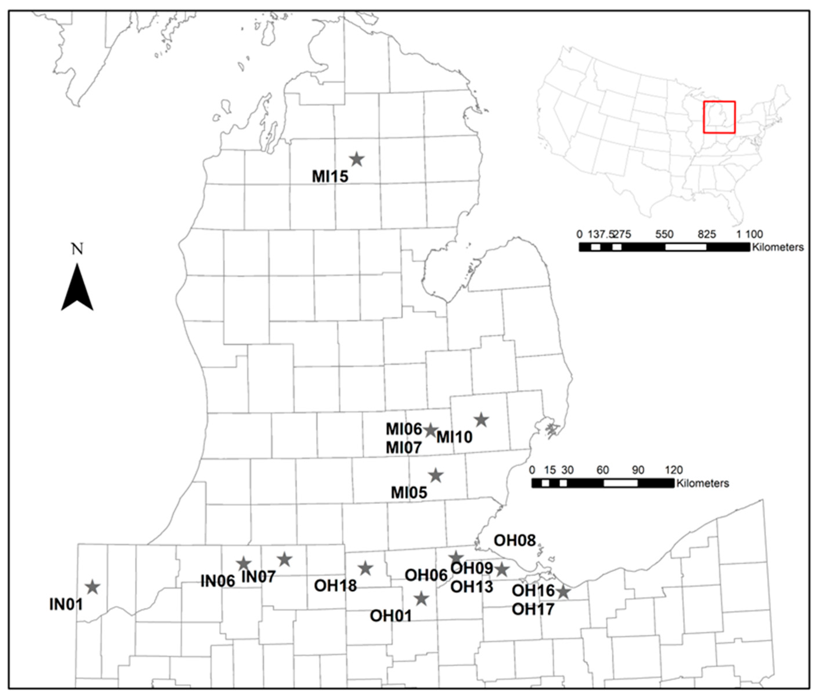
2.1. Samples and Genotyping

We conducted field sampling from April–August of 2019 to 2021 in the Lake Erie Watershed in southeast Michigan and northern Ohio. Field sampling in Indiana took place from March through July of 2017–2019 and a single locality in 2021. Additional samples from northern Michigan were obtained through a partnership with an ongoing study in the Kingsbury Lab. Trapping was conducted following the Northeast Blanding’s Turtle Working Group trapping protocol [35] (Appendix A). Blood was drawn from the nuchal sinus using IACUC-approved methods, preserved in 95% ethanol, and placed in a standard freezer until extraction. No more than 10% of the blood volume was drawn from any given individual. For samples collected during the 2017–2019 seasons, tail clippings were collected instead of blood.
We extracted DNA from 95 microliters of alcohol-preserved blood and tissue (Appendix A) using the Qiagen DNeasy Blood and Tissue extraction kit (Valencia, CA, USA). Fifteen microsatellite markers and primers were chosen from prior studies to maximize genetic variation and facilitate cross-regional comparison for future study (Table S1). These loci were chosen for their number of alleles, ability to be multiplexed, and high degree of use across regions [36]. These microsatellite markers were developed for a variety of turtle species and have been used on E. blandingii across their geographic range [26,30,37,38,39,40,41,42]. PCR reactions were performed using a Qiagen Multiplex PCR Kit (Valencia, CA, USA) following manufacturer protocol. We then sent PCR products to the Yale DNA Analysis Facility or the Yale Keck DNA Sequencing Lab for fragment analysis. All samples were run on an Applied Biosystems 3730xl 96-Capillary Genetic Analyzer using the GelCo. Liz 500 size standard. We analyzed electropherograms using Geneious v. 11.1.5; all loci were scored and binned based on the expected number of repeats. Each locus was rerun at least once with a replicate sample to establish confidence in allele scoring. For thermocycling conditions, see Appendix A.

2.2. Analysis within Localities

We used GenAlEx 6.5 to check raw data for missing values and export data into different formats [43]. Within sample localities, we tested for deviation from the Hardy Weinberg equilibrium using PopGenReport [44] and linkage equilibrium among all locus pairs in Genepop version 1.1.7 [45]. PopGenReport was further used to determine the relationship between allele numbers and sample size per location, screen for null alleles, identify private alleles, and determine allelic richness with rarefaction [44].
Overall, we collected 492 samples from 49 localities. Initially, we ran PopGenReport with all sites regardless of sample size to assess the relationship between number of alleles and sample size to set a minimum sample size for estimates of allelic richness and the number of private alleles. Some localities had large samples sizes (>70). To avoid bias in estimates of genetic variation in comparison to localities with smaller samples, we randomly sub-sampled these localities to a maximum of thirty individuals [46]. Ultimately, we ran descriptive statistics for all sites with at least ten samples and a maximum of thirty samples. These localities ranged from across northern Indiana into the Lake Erie Marshes of Ohio and southeastern Michigan, with one locality in northwest Michigan (Figure 1). Additionally, we ran these descriptive statistics for the clusters derived from TESS3r to provide a historic perspective in the presence of geneflow (See Table S6).
We used DiveRsity Version 1.9.90 to estimate genetic diversity within sample localities using observed heterozygosity (HO), Nei’s expected heterozygosity (HE), FIS and allelic richness. We tested for differences in allelic richness among sites using a linear mixed model followed by Tukey post-hoc tests of pairwise differences. We also calculated FST and Jost’s D [47] to assess the level of differentiation among sample localities.
BOTTLENECK version 2.2.02 uses each population and loci to examine the expected versus observed heterozygosity relative to the number of individuals and alleles used in each population [48,49,50]. We used BOTTLENECK parameters following Davy and Murphy [51], a study that had similar sample sizes and numbers of locations and loci for a similar long-lived species of turtle. We ran BOTTLENECK using a two-phase model replicated 1000 times to check for evidence of population bottlenecking. Variance in the model was set at 12% and the single-step mutation rate was set at 95%, whereas the multistep mutation rate was set to 5%.
It is important to understand the number of individuals in a population that are contributing to the next generation (effective population size, Ne) [52,53,54]. We used NeEstimator Version 2.1 to assess the effective population size of each site. NeEstimator uses linkage disequilibrium under a molecular co-ancestry method to determine the Ne and also provides jackknifed confidence intervals [55,56]. We ran NeEstimator with the Linkage Disequilibrium random mating model. To evaluate the impact of sample size on Ne estimation, we ran NeEstimator using three different randomly generated sub-samples from the largest site (OH-08): one with 10 individuals (our N cut off), one with 30 individuals (or N max), and one with 77 individuals sampled. Additionally, we ran BOTTLENECK and NeEstimator for the clusters derived from TESS3r to provide a historic perspective in the presence of geneflow (See Table S7).
We also used Bottlesim v. 2.6 to explore the impacts of potential future bottlenecks in the absence of gene flow [57]. Bottlesim was run for our largest census population OH-08 with the following assumptions: initial population size of 200 for all scenarios, a 1:1 sex ratio, dioecy with random mating, and diploid multilocus individuals. Longevity was set to 65, and age of maturity was set to 14 following Anthonysamy et al. [30]. In the first scenario, the population declined 50% over 200 years, and the second scenario saw a 90% population decline. Both scenarios were explored using 1000 replicates.

2.3. Population Structure

Geographic distance has been identified as potential driver of population structuring in E. blandingii [26,28]. We ran a Mantel test using Adegenet [58] in R to test for isolation by distance among pairs of individuals using 9999 permutation and pairwise chord distances [59].
We further investigated population structure using a range of approaches to genetic clustering, including methods implemented in STRUCTURE version 2.3.4 [60], TESS3r version 1.1.0 [61], and Adegenet version 2.1.4 [58]. Population structure analysis is used for identifying populations and management units for a species without relying on sample location a priori. By using multiple methods, concordance in inferred clustering gives higher confidence in attributing results to a biological process. Additionally, genetic clustering is often hierarchical and using multiple methods can help to determine finer scale patterns among broader clustering schemes. Areas of disagreement in clustering between methods can also highlight areas where clear population structure is difficult to discern and may require additional sampling and analysis.
STRUCTURE Version 2.3.4 uses a Bayesian cluster analysis method that relies on Markov Chain Monte Carlo (MCMC) to group individuals into clusters using unlinked genetic markers [43]. STRUCTURE is a model-based approach that uses the frequencies of each allele at each locus to probabilistically assign individuals to a given population/cluster (K) based on shared allelic frequency while also avoiding departure from HWE and LDE within assumed populations [60,62]. Assuming an admixture model within STRUCTURE allows individuals to be assigned to one or more populations by utilizing a Q matrix that compares the proportion of an individual’s genome associated with a given assumed population [60,62]. We ran STRUCTURE 10 times for K values from 1 to 10, where each run had a burn-in of 50,000 proceeded by 100,000 steps. We implemented the LOCPRIOR function in all runs. LOCPRIOR is a function that incorporates sample locations as a priori information, a method that has been shown to assist with the identification of clusters when differentiation is weak [63]. We viewed STRUCTURE results using STRUCTURE Selector [64], which allows the visualization of the STRUCTURE results in a bar graph format using the Puechmaille method (controls for uneven sampling size) and provides graphic representations of the ΔK and MedMeaK/MedMedK selection criteria [65]. Initially we examined the results using a 0.5 threshold level (Figure S2), which is the default; however, since Puechmaille (2016) recommends investigating different threshold levels to assess its effect on clustering, we focused on a 0.8 threshold level. The bar graph displays individual assignment to each given cluster represented by the different colors. Although ΔK methods are commonly presented, MedMeaK/MedMedK is more robust when sampling is uneven [65] and so only those values will be presented here.
TESS3r also implements admixture models and MCMC but incorporates spatial information and autocorrelation into the prior distribution of the Q-matrix by allowing admixture of each individual to change across geographic space (individual ancestry) [62]. Individual variation in admixture also decreases at a regional and local level to allow for clines in all directions [62]. In addition to the Q-matrix, TESS3r also uses a G-matrix that includes the ancestral genotypic frequencies to conduct a combination of matrix factorization and quadratic programing to determine the number of clusters present in the given data set [61]. Francois and Durand [62] have demonstrated that Bayesian approaches that incorporate geographic priors (TESS3r and STRUCTURE LOCPRIOR) are more advantageous at detecting accurate population structure. Additionally, Francois and Durand [62] demonstrated that TESS3r does a better job at capturing the geographic driven clustering than STRUCTURE. TESS3r and STRUCTURE with LOCPRIOR have been shown to effectively predict population structure in organisms that have experienced high degrees of glacial driven expansion and contraction [62]. TESS3r also allows results to be visualized over geographical space as well as in a traditional bar graph format [61]. We ran TESS3r for K = 1 to 10, and the number of clusters (ancestral populations) was determined using cross-validation criteria.
We utilized Adegenet version 2.1.4 to perform a spatial Principal Component Analysis (sPCA) [58]. A sPCA is a spatially explicit multivariate approach to determine genetic structure between populations [66]. sPCA uses a connection network to identify which populations are neighbors and which are not; the neighboring populations are then compared using allelic frequencies [66]. sPCA then uses the spatial autocorrelation and variance of allelic frequencies to search for genetic correlation over geographic space using Moran’s I [67]. We created a connection network using the overlap in home range (2 times the radius) between individuals [68]. We used a regional estimate for home range size of 37 hectares [69]. The sPCA looks to uncover local and global structure, where local structure represents higher genetic differentiation between neighbors in a connection network than between random individuals, and global structure represents the differences between spatial groups or clines [66,70].
An important aspect of understanding observed genetic composition is determining which populations have interacted with each other, and the extent and direction in which gene flow has occurred. Understanding migration patterns can help inform historic and current source-sink dynamics, which may make some populations less stable than others. Since we were primarily interested in movement between populations/management units due to their potential application in conservation, site localities were grouped into the four clusters identified by TESS3r (Table S3). TESS3r was chosen because it produced conservative population clusters, and has been indicated to be most robust for detecting effects of multidirectional clines into clustering compared to STRUCTURE [62].
Migrate version 4.4.3 was used to examine rates of historic migration between clusters to determine the degree to which clusters have historically interacted [71]. Migrate uses a Brownian motion approximation stepwise mutation model as well as Bayesian inference to determine effective population size and past migration rates [71]. Migrate assumes a migration matrix model that uses asymmetric migration rates and assumes different sub-population sizes with population divergence and admixture present. Migrate was run using a Brownian motion model with priors for theta (Θ) set from 0–1000. Simulations used one long chain with sample increments of 200 and recorded 5000 steps per chain after a burn in of 1000 steps. To extend the length of the run and allow for greater convergence, a multiple Markov chain statistical heating scheme was used with four chains with temperatures of 1.00, 1.50, 3.00, and 1,000,000.00, respectively, with the swapping interval set to 1. The long term gene flow estimates from Migrate were then converted to average proportion of migrants using the formula: mi→j = (Mi→j)(μ) so that it would be comparable to the BayesAss estimates [32]. Goldstein et al. [72] provided a mutation rate of 5.6 × 10⁻⁴, which was used for μ [32,72]. BayesAss edition 3 (BA3; [73]) was used to examine more recent (the past few generations) levels of migration between the same four TESS3r clusters used in Migrate. BayesAss takes a Bayesian approach to estimating recent migration using MCMC to estimate posterior probabilities [73]. BayesAss allows for population-internal frequencies to deviate from HWE and uses the temporary states of disequilibrium to make inferences about recent population gene flow [73]. Input files for BayesAss were formatted using Formatomatic [74]. BayesAss was initially run with 10,000,000 iterations of the MCMC chain utilizing a burn in of 1,000,000 and a sampling frequency of 1000. These initial parameters did not allow for proper convergence of the Markov Chain, so the number of iterations was increased to 1,000,000,000. Tracer v1.7.2 was used to calculate 95% confidence intervals and to view trace files from BayesAss [75].
The directionality of gene flow and source sink dynamics were calculated for the mean historic migration rate from Migrate and for the mean recent migration rate from BayesAss. Net emigration was calculated by subtracting the total immigration from the total emigration for each cluster.

3. Results

3.1. Tests of Equilibrium

Out of 224 tests of HWE, GmuD40 showed deviation at one locality (OH-17). Because this single locality at one locus is unlikely to impact the multilocus analysis, we retained the locus for subsequent analysis. GmuD28 and GmuD107 (p ≤ 0.0001) showed significant linkage disequilibrium after Bonferroni correction. We removed GmuD28 from further analysis, and GmuD107 was retained.

3.2. Analyses within Localities

One hundred and sixty-nine alleles were detected across the remaining 14 loci, representing 16 sample localities and a total of 313 individuals (Table 1). The number of alleles per locality ranged from 68 to 97 across loci and increased according to the number of individuals sampled (Table 1). The number of alleles by sample size at a location appears to have reached or come close to an asymptote, with sites having around 20 individuals having nearly the same or more alleles than the largest samples (n = 30) (Figure S1). Of the 315 individuals and the 14 microsatellites used, 1.51% of the genotype data was missing. The number of private alleles ranged from 0 to 7 for the sites with at least 10 samples (Table 1). Of the 14 loci used for analysis, GmuD79 was monomorphic and uninformative, leading it to be omitted for analysis, leaving us with 13 informative loci.
Mean allelic richness ranged from 4.01 to 4.84, but there was no statistical difference between localities (Table 1). Observed heterozygosity across sites ranged from 0.58 to 0.65 (Table 1). FIS values indicated no evidence of inbreeding among sites; however, there is potential outbreeding in MI-6 and MI-10 (FIS < 0 for the bootstrapped 95% confidence interval). Overall FST was 0.05 (pairwise FST = −0.01–0.15) and overall D was 0.08 (pairwise D = 0.00–0.17). The FST and D values showed isolation by distance (Table S2).
No bottlenecks were detected in most localities; however, a Wilcoxon test suggested heterozygosity excess in OH09. Conversely, sign tests indicated heterozygosity deficiency in IN01, MI06, OH01, and OH16 (Table 2). Effective population size estimates ranged from 7.9 to ∞ (Pcrit = 0.05) and 8.5 to ∞ (Pcrit = 0.02) (Table 2). However, effective population size estimates decreased with increasing sample size and produced confidence intervals with an upper limit (Table 2 & Table 3).
Projection of genetic variation 200 years into the future showed a ~9% loss of alleles under a constant population size, a ~17% loss of alleles under a 50% population reduction, and a >50% reduction in alleles in a 90% population reduction (Figure 2a). Loss of HO was less than 15% regardless of the effective size loss modeled (Figure 2b).

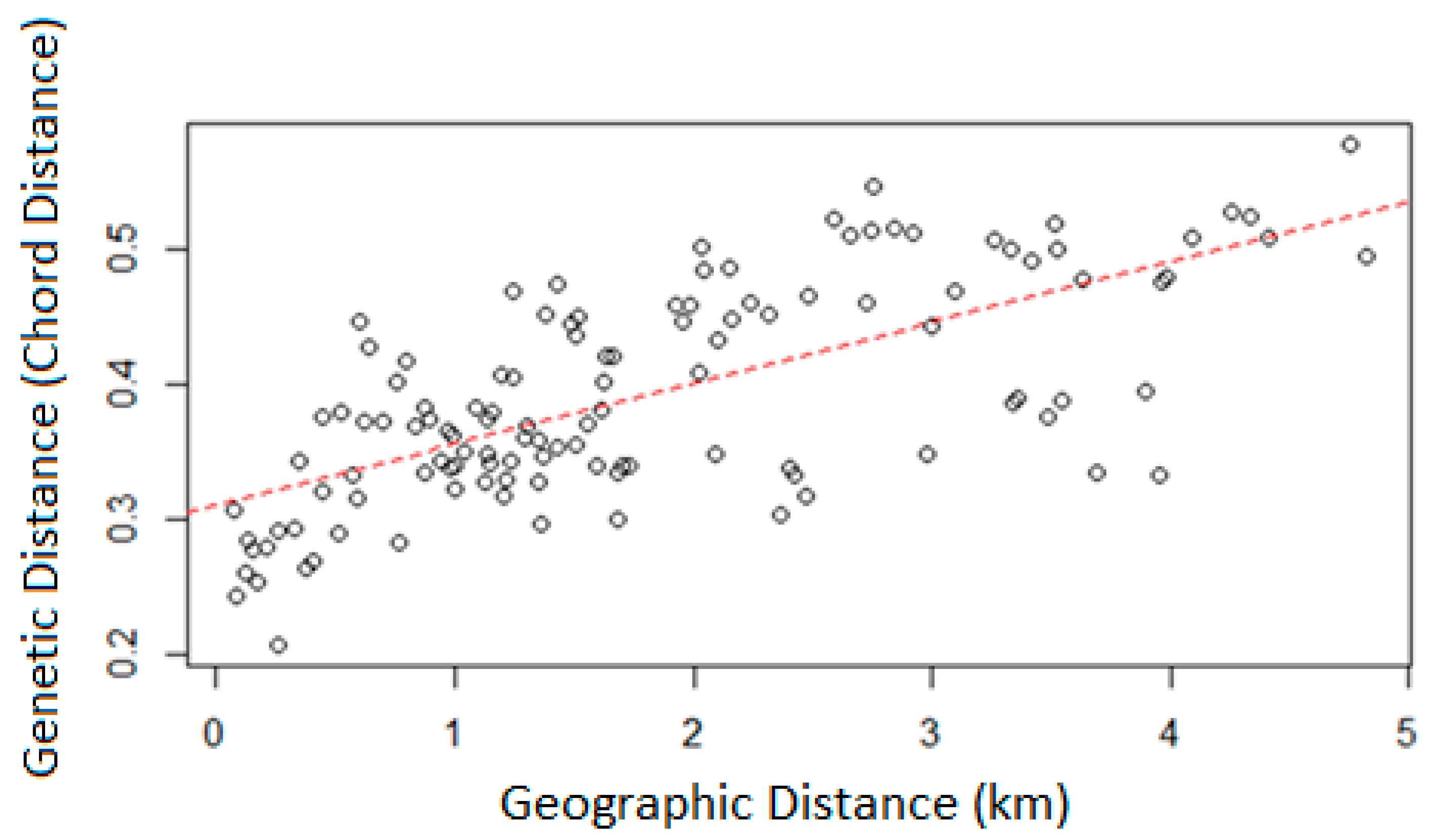
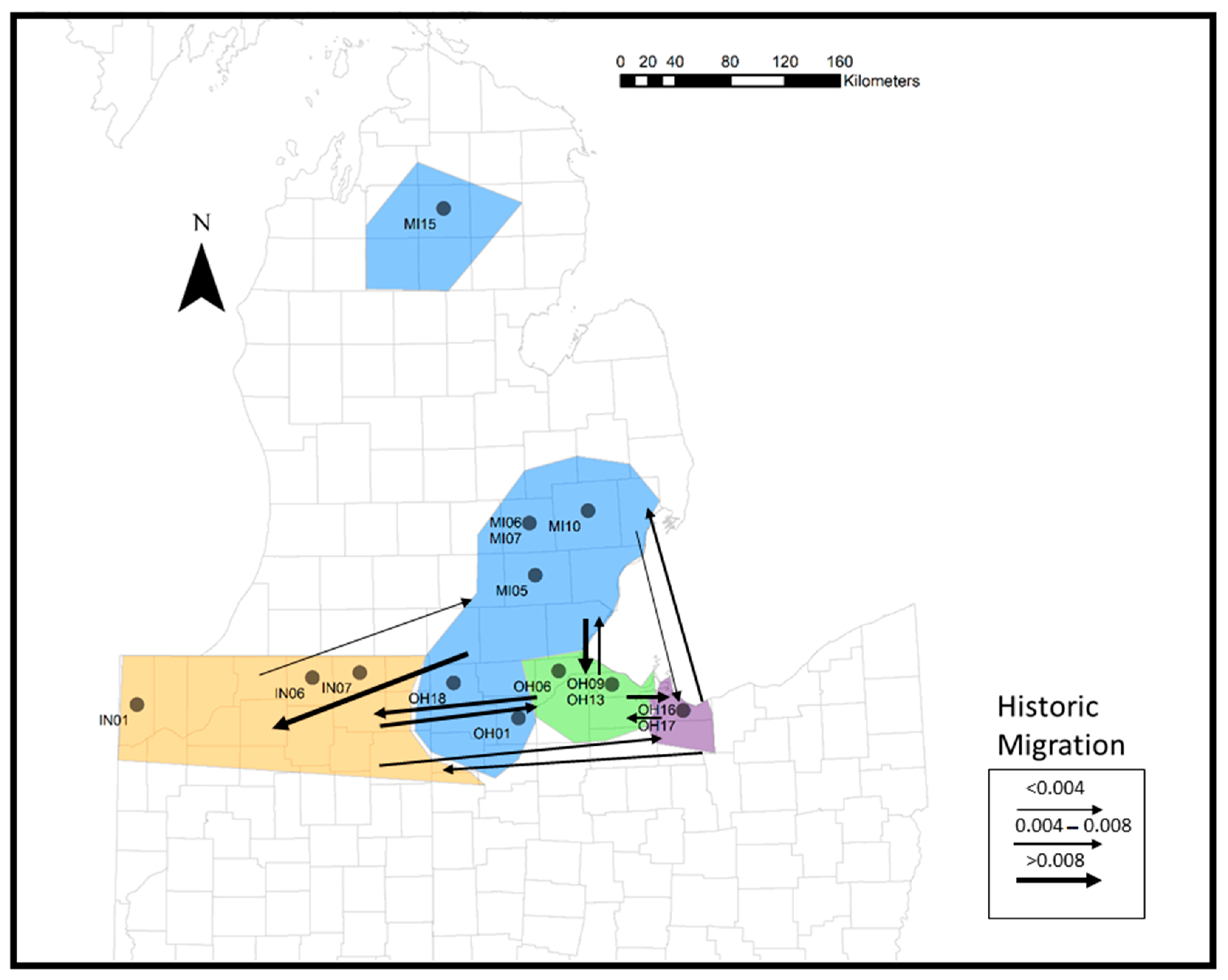
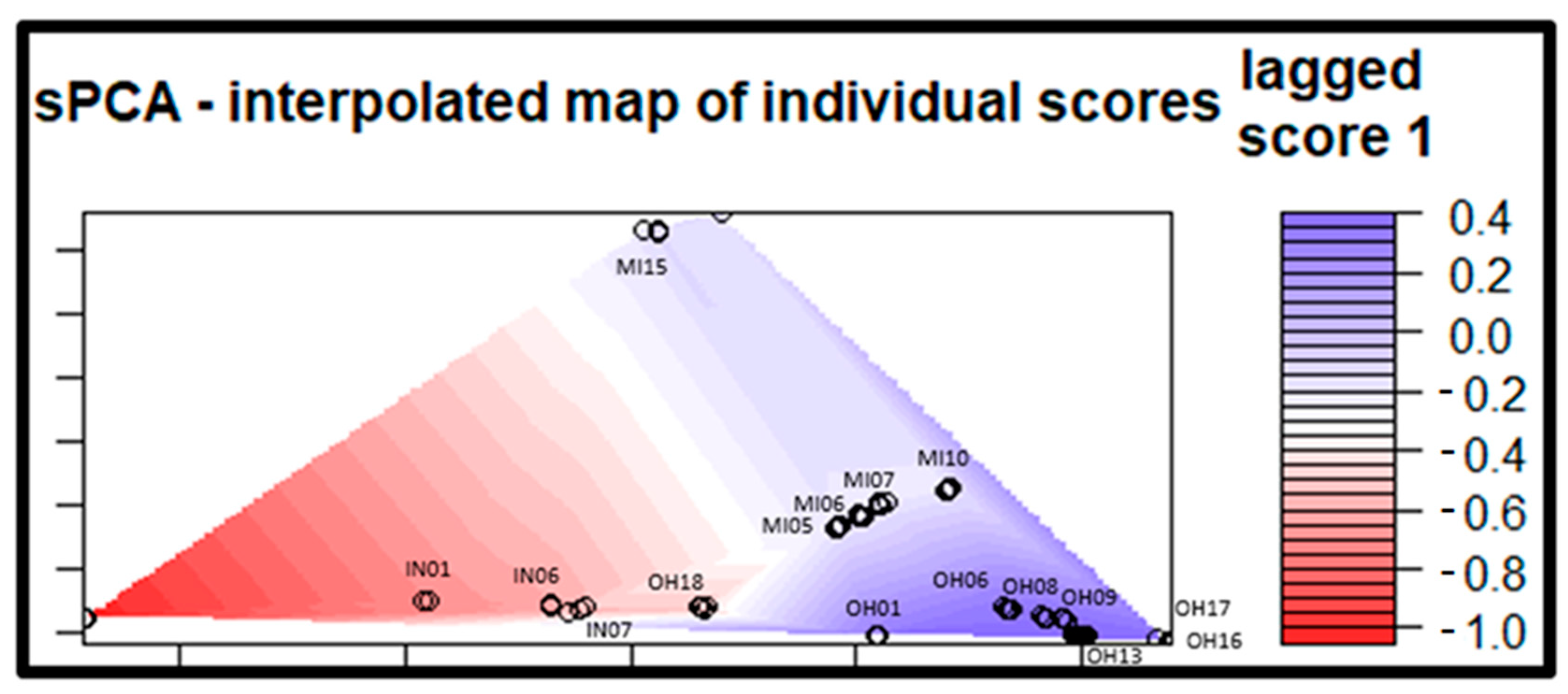
3.3. Population Structure

The relationship between pairwise geographic and genetic distance (Edwards Chord Distance) was positive (Mantel variance = 0.69, r2 = 0.31, p < 0.0001) (Figure 3 and Figure S5).
Clustering varied depending on assumptions made in the analyses. We viewed the STRUCTURE results under a 0.8 threshold level, which uncovered a K = 4 for the MedMedK and MaxMedK similar to TESS3r, which also identified K = 4 using cross-validation scores (Figure S3). The K = 4 clustering scheme produced by STRUCTURE was very similar to TESS3r in grouping IN01, IN06, IN07 together, MI05, MI06, MI07, MI10, MI15, OH18, OH01 together, and grouping OH06, OH08, OH09, OH13 together (Figure 4a,b). The STRUCTURE K = 4 scheme differed from TESS3r by clustering OH16 on its own and OH17 with OH06-OH13. TESS3r created a more gradual west–east cluster pattern compared to STRUCTURE (Figure 4 and Figure 5). TESS3r clustered OH16 and OH17 together as one cluster apart from all other localities, refining the east to west trend indicated by STRUCTURE (Figure 4a,b).
Since the first two principal component axis of the spatial PCA explained most of the variance, only those principal components were maintained. The first and second principal component explained 55.92% and 7.00% of the spatial genetic structure, respectively. Significant global structure was observed across all localities (r = 0.019, p = 0.007), whereas no local structure was observed (r = 0.009, p = 0.797). With the first two PCA axes retained, two clusters were identified, with all three Indiana localities grouping together along with OH-18, and all the Ohio localities grouping together. The Michigan localities were intermediate in between the Ohio and Indiana localities (Figure 5 and Figure S4).
Mean historic mutation scaled migration rates ranged from 6.90 to 20.20 (or 23.86 and 102.56 individuals per four generations) with the highest rate of average migration being from cluster 2 to cluster 4, and the lowest average migration rate being from cluster 1 to cluster 2 (Figure 5 and Table S4). The mean historic migration rate ranged from 0.0038 to 0.011 and none of the 95% confidence intervals included zero (Table S4). Mean recent migration rates ranged from 0.08 to 0.09; however, all values included zero at the 95% confidence interval, indicating little to no recent migration (Figure 5 and Table S3). For mean historic migration, cluster 2 acted as a source for clusters 1, 3, and 4. Since mean recent migration was not significant, the source sink values were not included here (Table S5).

4. Discussion

4.1. Analyses within Localities

Understanding levels of genetic variation in the context of demographic history and species life history is fundamental to the management of populations [76]. Our examination of genetic variation of E. blandingii across Indiana, Ohio, and Michigan shows high levels of within locality genetic diversity across localities (Table 1) that is comparable to that found in most populations range wide (Table 4). There is not consistent evidence of recent bottlenecks at any locality (Table 2). Some localities showed low p values but had more heterozygosity deficiency than excess, indicating possible outbreeding similar to what Anthonysamy et al. [30] found in Illinois (Table 2). Ohio had a single locality (OH-09) that had a significant p value (<0.05) for the Wilcoxon test but did not show significant excess in the sign test (Table 2). These results are somewhat paradoxical given the fragmentation of habitat and small population sizes that are characteristic of Blanding’s turtle populations outside of Nebraska and Minnesota [6].
There are two interrelated factors that likely account for the high standing levels of genetic variation we observed. First, long and overlapping generations have been shown to reduce the sensitivity of populations to genetic loss following recent population decline in freshwater turtles [25,51,77] and other long-lived species [78]. Blanding’s turtles can live more than 85 years and have generation times of 37 years, both of which are among the longest of any freshwater turtle [2]. These life history characteristics should buffer populations from genetic bottlenecks. Second, gene flow assists with the maintenance of local genetic variation. Our estimates of gene flow suggest that it was higher in the past (Table S4), a result that aligns with previous work on the species [28].
To investigate the future prospect genetic variation, we used genotypes from one of the larger census populations to simulate allelic richness and heterozygosity for 200 years under three scenarios of population change [57]. The model used accounts for overlapping generations in an isolated population of 200 individuals undergoing random genetic drift. We deemed these assumptions appropriate given the low contemporary gene flow, habitat isolation, and typical size of current populations [79]. The results show a steady loss of genetic diversity over 200 years, even with a constant population size. A more likely scenario for many populations is the 90% decline, which results in a loss of half of standing genetic variation. Few juveniles were observed in the field and E. blandingii are long-lived organisms with high nesting mortality; therefore, it is possible that several of the sampled localities may have “ghost” populations consisting of a handful of long-lived adults [80] that see little to no recruitment. This analysis suggests that the currently high levels of genetic variation observed are a misleading measure of genetic security in populations.
Our estimates of effective population size also suggest that populations are small, and at risk of inbreeding depression in the short term (Ne < 50) and loss of evolutionary potential long term (Ne < 500) [81,82]. Before interpreting the results, we recognize that estimates of Ne from a single genetic sample are often biased and have low precision [83], especially in species with overlapping generations [84]. Moreover, we found that the sample size of individuals influenced estimates; lower Ne and greater precision was found with increasing sample size (Table 3). When an Ne estimate was available for a locality (not infinity and requiring both Ne estimates from each Pcrit to meet a size threshold), values were <500 in 7 of 16, and <50 in 3 of 16 localities, respectively (Table 2). Because samples sizes were 30 or less, we anticipate that values are actually lower than these estimates due to the upward bias we observed with a small sample size (Table 3). Further work is needed to refine these estimates and explore the use of effective number of breeders (Nb) per year, a related metric that is more tractable for detecting population decline in species with long generation times [85]. However, the available information indicates that several populations appear to be at immediate risk of inbreeding depression and would benefit from assisted gene flow [82].

4.2. Population Structure

Determination of population structure is important for identifying units for conservation and developing strategies for possible translocation of individuals that reduces the risk of outbreeding depression. We find that genetic differentiation is generally low among localities overall (FST = 0.05, D = 0.08), an observation that reflects most studies conducted at a regional scale (Table 4). Although there was statistically significant pairwise differentiation in several comparisons (Table S2), we did not find strong differences in structure over short distances, as has been reported in some Illinois and New York populations [28,30]. Rather, there was a strong pattern of isolation by distance across localities (Figure 3) with the greatest pairwise differentiation occurring between IN-01 (western most locality) and OH-17 (second most eastern site) (FST = 0.15, D = 0.21, Table S2).
The number of genetic clusters identified through each method ranged from K = 2 to K = 7 (sPCA, STRUCTURE). We observed that higher K values from STRUCTURE are representative of hierarchical clustering or sub-structures that fall within the broader clusters identified by TESS3r. Under multiple schemes we consistently identified clusters including IN-01, IN-06; M-I05, MI-06, MI-07, MI-10, MI-15; and OH-06, OH-08, OH-09, OH-13. This suggests that these groupings might represent historical or ecological significance. Given this result and the observation that differentiation across sites was low as noted above, we interpreted fewer inferred clusters as having greater likelihood of capturing the overall trend of population differentiation.
Despite the overall weak signal for structure regardless of the method employed, our results provide support to prior findings that E. blandingii are not in panmixia across the Midwest and Great Lake Regions (Table 4) [10,26,27,28,29,30]. We follow others in suggesting that the observed pattern of differentiation is due to palaeoecological landscape change that occurred prior to the more recent modifications caused by European settlement over the past 300 years [7,28]. Weak differentiation is likely due to rapid range expansion from southern refugia into formerly glaciated areas once ice began to recede ~15,000 years ago, and subsequent differentiation as major watersheds developed [28,86]. Within our study area, sampling occurred in portions of the Lake Michigan and Lake Erie watersheds [level hydrological unit code 4 (HUC 4), United States Geological Service]. sPCA analysis recovered two groups generally aligned with the watershed boundary (Figure 6) as did TESS3r, but with further sub-structuring within the Lake Erie region (Figure 5). Moreover, our historic or long-term gene flow estimates were relatively high compared to contemporary estimates using BayesAss (Figure 5). This suggests a degree of connectivity in the past which would act to minimize differentiation across the landscape, a pattern that is consistent with other studies of gene flow in the species [28,32]. Additional sampling throughout Michigan would help to better resolve the pattern and allow tests of the historic dispersal of lineages and their pre-settlement connectivity following deglaciation.

4.3. Conservation Implications

Identification of a minimum viable population size is of interest to guide management for individual populations, the most fundamental level at which conservation decisions are made. Although controversial [81,87], the 50/500 [88] rule sets a lower limit for Ne from a genetic perspective for the short-term avoidance of inbreeding depression and long-term risk of genetic drift, respectively. Except for a few notable exceptions, census sizes of Blanding’s Turtle populations tend to number in the tens to hundreds of adults [6,78]. Ne is often much lower than the population census size (Nc) for wild populations (~10–20% across taxonomic groups) since Ne accounts for sex ratio, variation in reproductive success, and variation in population size [54]. However, our best estimate of Ne (137.1 for OH-08) was close to the adult census size (174 assuming a 1:1 sex ratio) estimated by Cross et al. [89] at the locality, giving an Ne/Nc ratio of 0.79. Higher ratios such as these are not uncommon in long-lived taxa with overlapping generations [84,90]. Although it is a single estimate and more work is necessary to establish certainty, the data suggest that Ne/Nc ratios for the species and the census size may reasonably approximate numbers for the minimum viable population size.
Even so, several populations are currently <50 adults (Table 2), the most concerning value for resilience in the immediate future [91]. Using population viability analysis (PVA), King et al., (2021) estimated the minimal initial population size with an extinction probability of <5%, and then used this value to determine that a population size of ≥50 adults was needed to maintain expected heterozygosity of 95% for 100 years under a scenario including catastrophes. A population of this size with at least 100 ha of habitat and a growing or stable population size was considered resilient based on census size [92], resulting in a threshold Ne of ~40 based on the Ne/Nc ratio above. We corroborated these estimates with a modelling approach that uses genetic rather than demographic data to simulate future genetic variation (Figure 3). Under the Bottlesim model, a population dropping to Ne = 100 would retain 98% HO, while a population dropping to Ne = 20 would retain 95% HO and experience a much greater loss in number of alleles over 100 years. It should be noted that this modelling approach does not account for differential reproductive success or survival based on the age of the individuals, environmental stochasticity, or low recruitment, features seen in E. blandingii [2,6,52,93]. Therefore, excluding life stage dynamics in Bottlesim models likely leads to under-estimation of the genetic impacts resulting from population reductions in the absence of gene flow. Given that gene flow is currently restricted in our study area (Table S4) and elsewhere (summarized in King 2023 [92]), the results of PVA and Bottlesim modelling approaches within populations suggest that several populations are at risk of inbreeding depression and that assisted gene flow [82] and/or population augmentation [94,95] is warranted in many cases.
Levels of genetic variation are currently robust within the species across the geographic range (Table 4). This provides an opportunity to strategically manage populations to avoid the expected future loss of genetic variation in small, isolated populations. First, it is necessary to identify large, relatively stable or growing populations that occur in large tracts of suitable habitat [92]. These populations can serve as a source of individuals for translocation to other localities that have habitat sufficient to support viable populations. Our results suggest that genetic structure should be a minor concern for translocation. If possible, source and recipient populations should share the same watershed at the level of HUC 4 (above and [92]). However, the minimal structure between watersheds and the overall history of recolonization following deglaciation suggests that movement of turtles between watersheds will carry little risk of outbreeding depression within phylogeographic regions [7,10]. In this case, we suggest that source and recipient populations are chosen to maximize geographic proximity (isolation by distance) and environmental similarity to avoid possible disruption of co-adapted gene complexes [96].

5. Conclusions

Observed levels of within locality genetic diversity and the lack of bottleneck detection implies a level of genetic security within the Great Lakes Region. However, the observed diversity may be representative of remnant population structure and historic gene flow masking ongoing or developing bottlenecks and a potential forthcoming decline in genetic diversity [25]. Conservation strategies such as head-starting, translocation, and habitat protection can help to combat loss of genetic diversity and prevent future bottlenecks [97,98].
The observed population structure provides an initial basis to guide translocations or head-starting among localities. Since the genetic clusters generally show a weak signal and differentiation between localities was relatively low, the risk for outbreeding depression is likely minimal, though the closest source locality would provide the lowest risk (since IBD was detected) [97,99]. In this scenario, minimum viable population size, population demographics, and risk of disease transmission is more important for determining a source population for translocation [79,100,101,102].
Our findings support the currently reported genetic trends observed in E. blandingii across their range; although genetic differentiation is low between localities, there is genetic structure [10,26,27,28,29,30]. Further sampling and analysis and a range wide scale using microsatellite and genomic markers would help to further understand the genetic trends and historic drivers of population structure within E. blandingii.

Supplementary Materials

The following supporting information can be downloaded at: https://www.mdpi.com/article/10.3390/d15050668/s1, Figure S1: Number of alleles detected at locality versus sample size by locality; Figure S2: MedMeaK and MedMedK STRUCTURE bar graphs; Figure S3: Cross validation score; Figure S4: Spatial Principal Component Analysis; Figure S5: Histogram of Mantel test; Table S1: Summary of fifteen microsatellite loci; Table S2: Pairwise FST and D; Table S3: Locality Cluster Assignment; Table S4: Migration & BayesAss; Table S5: Total and Net Immigration and Emigration; Table S6: Summary of descriptive statistics by Cluster derived from TESS3r; Table S7: Summary of Bottleneck tests and effective population (Ne) at the 0.05 and 0.02 Pcrit values size estimates with 95% confidence intervals.

Author Contributions

Conceptualization, M.C., G.L.J., Y.L., D.G. and M.J.; methodology, D.G. and M.J.; software, D.G.; formal analysis, D.G. and M.J.; investigation, D.G., C.D., D.E. and J.H.; resources, M.C., G.L.J., Y.L., B.K. and M.J.; data curation, D.G., M.C., G.L.J., Y.L., D.E., C.D. and J.H.; writing—original draft preparation, D.G.; writing—review and editing, D.G., M.J.; visualization, D.G.; supervision, M.C., G.L.J., Y.L., B.K. and M.J.; project administration, M.C., G.L.J., Y.L., B.K. and M.J.; funding acquisition, M.C., G.L.J., Y.L., B.K. and M.J. All authors have read and agreed to the published version of the manuscript.

Funding

This research was funded by Indiana Department of Natural Resources State Wildlife Grant T7R21, Toledo Zoo, and the United States Fish and Wildlife Service Competitive State Wildlife Grant F19AP00159.

Institutional Review Board Statement

Turtle protocols were approved by the Animal Care and Use Committees of Purdue University (1112000451), Ohio State University (2015A00000005), and Michigan State University (PROTO202000132/AMEND202200506), as well as by the Toledo Zoo Research Review Board (#R-1801).

Data Availability Statement

Data are available upon request following the policies of the respective state wildlife agencies.

Acknowledgments

I’d like to thank the many field leads, field technicians, and volunteers who contributed to data collection and field sampling: Kailyn Atkinson, Chloe Bates, Julia Boldrick, Katie Brandewie, Charlotte Brennan, Morgan Boyer, Ian Chick, Elizabeth Cubberly, Connor Dempsey, Diana Digges, Dan Earl, Stephanie Emerine, Molly Fava, Nick Friedeman, Talia Greenblatt, Gia Haddock, Jessica Hinson, Beckie Hippensteel, Trevor Hoffman, Liz King, Minh Lee, John Lynch, Carly Martenson, Jen Mayer, Andrew Metz, Chrissy Mominee, Sophie Mills, Sean Obrochta, Elspeth Pierce, Zack Pitman, Shelby Priester, Trevor Proctor, Joseph Redinger, Mic Rohde, Courtney Ross, Dale Shank, Frank Schroyer, Jacob Schott, Tyler Scoville, Ayley Shortridge, Nick Smeenk, Hunter Smith, Jesse Sockman, Reine Sovey, Bria Spalding, Courtney Thompson, Jenny Swonger, and Megan Wise.

Conflicts of Interest

The authors declare no conflict of interests.

Appendix A

For the first trapping season in Ohio and Michigan, sites were chosen based on current observed or historic presence, along with habitat suitability. For the 2020 and 2021 trapping seasons, localities that fell within a circle with a 15 km radius were grouped into a genetic neighborhood. These genetic neighborhoods were intended to encapsulate the home range, breeding dispersal distance, and hatchling dispersal of E. blandingii at each locality [31,33,34]. We then focused on obtaining a minimum of 10 samples for at least one locality within an area presumed to be within the maximum movement distance of an individual Blanding’s Turtle. Indiana sites were chosen based on historical records [103]. Trapping was conducted using a combination of Hoop traps (~0.8 m diameter) and Promar traps (~0.3–0.5 m diameter).
Before starting extractions, stored blood was centrifuged and air-dried for ~15 min to separate and remove excess ethanol. A Nanodrop spectrophotometer was used to determine the concentration of extracted DNA. If sufficient DNA was not extracted and blood sample remained, the sample was re-extracted.
The 5′ ends of the forward primers were all tagged with universal florescent tails following the methods of Blacket et al., (2012) (6-Fam, NED, PET, or VIC) so that markers could be multiplexed in 5 reactions rather than 15 (Table S1) [36]. The concentration of the forward primers and universal tails differed slightly to optimize allele calls (Table S1).
Thermocycling included a denaturation step at 95 °C for 15 min, 35 cycles of denaturation at 94 °C for 30 s, annealing at 56 °C for 90 s, elongation at 72 °C for 60 s, and final elongation at 72 °C for 30 min. After thermocycling, completed samples were removed and stored at −80 °C. PCR was performed using 2 microliters of DNA (5–50 nanograms per microliter) in a 10-microliter reaction. Gel electrophoresis was performed for at least six samples from each round of PCR on a 2% agarose gel to ensure that amplification took place at expected product lengths.
Population bottlenecks tend to occur when populations experience a large reduction in effective population size, and results in a reduction in the number of alleles present among polymorphic loci [48]. A loss of alleles leads to a direct loss of genetic diversity, which can make a population more vulnerable to environmental change and stochasticity by constraining the available genetic plasticity [104]. When bottlenecks occur, the number of alleles present in a given population tend to drop more quickly than the expected heterozygosity, causing the expected heterozygosity to be greater than the observed heterozygosity (heterozygosity excess) [48].

References

  1. Lovich, J.E.; Ennen, J.R.; Agha, M.; Gibbons, J.W. Where have all the turtles gone, and why does it matter? BioScience 2018, 68, 771–781. [Google Scholar] [CrossRef]
  2. Congdon, J.D.; Dunham, A.; van Loben Sels, R. Delayed sexual maturity and demographics of Blanding’s turtles (Emydoidea blandingii): Implications for conservation and management of long-lived organisms. Conserv. Biol. 1993, 7, 826–833. [Google Scholar] [CrossRef]
  3. Kinney, O.M. Movements and Habitat Use of Blanding’s Turtles in Southeast Michigan: Implications for Conservation and Management; University of Georgia: Athens, GA, USA, 1999. [Google Scholar]
  4. Shaffer, H.B.; Minx, P.; Warren, D.E.; Shedlock, A.M.; Thomson, R.C.; Valenzuela, N.; Abramyan, J.; Amemiya, C.T.; Badenhorst, D.; Biggar, K.K. The western painted turtle genome, a model for the evolution of extreme physiological adaptations in a slowly evolving lineage. Genome Biol. 2013, 14, R28. [Google Scholar] [CrossRef] [PubMed]
  5. Joyal, L.A.; McCollough, M.; Hunter, M.L., Jr. Landscape ecology approaches to wetland species conservation: A case study of two turtle species in southern Maine. Conserv. Biol. 2001, 15, 1755–1762. [Google Scholar] [CrossRef]
  6. Congdon, J.; Graham, T.; Herman, T.; Lang, J.; Pappas, M.; Brecke, B. Emydoidea blandingii (Holbrook 1838)—Blanding’s turtle. Conserv. Biol. Freshw. Turt. Tortoises Chelonian Res. Monogr. 2008, 5, 015.011–015.012. [Google Scholar]
  7. Jordan, M.A.; Mumaw, V.; Millspaw, N.; Mockford, S.W.; Janzen, F.J. Range-wide phylogeography of Blanding’s Turtle [Emys (=Emydoidea) blandingii]. Conserv. Genet. 2019, 20, 419–430. [Google Scholar] [CrossRef]
  8. Avise, J.C.; Bowen, B.W.; Lamb, T.; Meylan, A.B.; Bermingham, E. Mitochondrial DNA evolution at a turtle’s pace: Evidence for low genetic variability and reduced microevolutionary rate in the Testudines. Mol. Biol. Evol. 1992, 9, 457–473. [Google Scholar]
  9. Alacs, E.A.; Janzen, F.J.; Scribner, K.T. Genetic issues in freshwater turtle and tortoise conservation. Chelonian Res. Monogr. 2007, 4, 107. [Google Scholar]
  10. Mockford, S.; Herman, T.; Snyder, M.; Wright, J.M. Conservation genetics of Blanding’s turtle and its application in the identification of evolutionarily significant units. Conserv. Genet. 2007, 8, 209–219. [Google Scholar] [CrossRef]
  11. Rödder, D.; Lawing, A.M.; Flecks, M.; Ahmadzadeh, F.; Dambach, J.; Engler, J.O.; Habel, J.C.; Hartmann, T.; Hörnes, D.; Ihlow, F. Evaluating the significance of paleophylogeographic species distribution models in reconstructing Quaternary range-shifts of Nearctic chelonians. PLoS ONE 2013, 8, e72855. [Google Scholar] [CrossRef]
  12. Parmley, D. Turtles from the late Hemphillian (latest Miocene) of Knox County, Nebraska. Tex. J. Sci. 1992, 44, 339–348. [Google Scholar]
  13. Holman, J.; Parmley, D. Noteworthy turtle remains from the Late Miocene (Late Hemphillian) of northeastern Nebraska. Tex. J. Sci. 2005, 57, 307–316. [Google Scholar]
  14. Spinks, P.Q.; Thomson, R.C.; McCartney-Melstad, E.; Shaffer, H.B. Phylogeny and temporal diversification of the New World pond turtles (Emydidae). Mol. Phylogenetics Evol. 2016, 103, 85–97. [Google Scholar] [CrossRef] [PubMed]
  15. Congdon, J.; Keinath, D. Blanding’s Turtle (Emydoidea blandingii): A Technical Conservation Assessment; USDA Forest Service, Rocky Mountain Region: Lakewood, CO, USA, 2006. [Google Scholar]
  16. Dahl, T.E. Wetlands Losses in the United States, 1780’s to 1980’s; US Department of the Interior, Fish and Wildlife Service: Washington, DC, USA, 1990.
  17. Ross, D.A.; Anderson, R.K. Habitat use, movements, and nesting of Emydoidea blandingii in central Wisconsin. J. Herpetol. 1990, 24, 6–12. [Google Scholar] [CrossRef]
  18. Grgurovic, M.; Sievert, P.R. Movement patterns of Blanding’s turtles (Emydoidea blandingii) in the suburban landscape of eastern Massachusetts. Urban Ecosyst. 2005, 8, 203–213. [Google Scholar] [CrossRef]
  19. Congdon, J.D.; Tinkle, D.W.; Breitenbach, G.L.; van Loben Sels, R.C. Nesting ecology and hatching success in the turtle Emydoidea blandingii. Herpetologica 1983, 39, 417–429. [Google Scholar]
  20. Prange, S.; Gehrt, S.D.; Wiggers, E.P. Demographic factors contributing to high raccoon densities in urban landscapes. J. Wildl. Manag. 2003, 67, 324–333. [Google Scholar] [CrossRef]
  21. Riley, S.P.; Hadidian, J.; Manski, D.A. Population density, survival, and rabies in raccoons in an urban national park. Can. J. Zool. 1998, 76, 1153–1164. [Google Scholar] [CrossRef]
  22. Ashley, E.P.; Robinson, J.T. Road mortality of amphibians, reptiles and other wildlife on the Long Point Causeway, Lake Erie, Ontario. Can. Field Nat. 1996, 110, 403–412. [Google Scholar]
  23. Congdon, J.D.; van Loben Sels, R.C. Growth and body size in Blanding’s turtles (Emydoidea blandingii): Relationships to reproduction. Can. J. Zool. 1991, 69, 239–245. [Google Scholar] [CrossRef]
  24. Frazer, N.B.; Gibbons, J.W.; Greene, J.L. Life tables of a slider turtle population. In Life History and Ecology of the Slider Turtle; Gibbons, J.W., Ed.; Smithsonian Institution Press: Washington, DC, USA, 1990. [Google Scholar]
  25. Kuo, C.-H.; Janzen, F.J. Genetic effects of a persistent bottleneck on a natural population of ornate box turtles (Terrapene ornata). Conserv. Genet. 2004, 5, 425–437. [Google Scholar] [CrossRef]
  26. Mockford, S.; McEachern, L.; Herman, T.; Snyder, M.; Wright, J.M. Population genetic structure of a disjunct population of Blanding’s turtle (Emydoidea blandingii) in Nova Scotia, Canada. Biol. Conserv. 2005, 123, 373–380. [Google Scholar] [CrossRef]
  27. Davy, C.M.; Bernardo, P.H.; Murphy, R.W. A Bayesian approach to conservation genetics of Blanding’s turtle (Emys blandingii) in Ontario, Canada. Conserv. Genet. 2014, 15, 319–330. [Google Scholar] [CrossRef]
  28. Sethuraman, A.; McGaugh, S.E.; Becker, M.L.; Chandler, C.H.; Christiansen, J.L.; Hayden, S.; LeClere, A.; Monson-Miller, J.; Myers, E.M.; Paitz, R.T. Population genetics of Blanding’s turtle (Emys blandingii) in the midwestern United States. Conserv. Genet. 2014, 15, 61–73. [Google Scholar] [CrossRef]
  29. McCluskey, E.M.; Mockford, S.W.; Sands, K.; Herman, T.B.; Johnson, G.; Gonser, R.A. Population Genetic Structure of Blanding’s Turtles (Emydoidea blandingii) in New York. J. Herpetol. 2016, 50, 70–76. [Google Scholar] [CrossRef]
  30. Anthonysamy, W.; Dreslik, M.; Douglas, M.; Thompson, D.; Klut, G.; Kuhns, A.; Mauger, D.; Kirk, D.; Glowacki, G.; Douglas, M. Population genetic evaluations within a co-distributed taxonomic group: A multi-species approach to conservation planning. Anim. Conserv. 2018, 21, 137–147. [Google Scholar] [CrossRef]
  31. Smith, P.W. An analysis of post-Wisconsin biogeography of the Prairie Peninsula region based on distributional phenomena among terrestrial vertebrate populations. Ecology 1957, 38, 205–218. [Google Scholar] [CrossRef]
  32. Howes, B.J.; Brown, J.W.; Gibbs, H.L.; Herman, T.B.; Mockford, S.W.; Prior, K.A.; Weatherhead, P.J. Directional gene flow patterns in disjunct populations of the black ratsnake (Pantheropis obsoletus) and the Blanding’s turtle (Emydoidea blandingii). Conserv. Genet. 2009, 10, 407–417. [Google Scholar] [CrossRef]
  33. Osentoski, M.F. Population Genetic Structure and Male Reproductive Success of a Blanding’s Turtle (Emydoidea blandingii) Population in Southeastern Michigan; University of Miami: Coral Gables, FL, USA, 2001. [Google Scholar]
  34. McGuire, J.M.; Scribner, K.T.; Congdon, J.D. Spatial aspects of movements, mating patterns, and nest distributions influence gene flow among population subunits of Blanding’s turtles (Emydoidea blandingii). Conserv. Genet. 2013, 14, 1029–1042. [Google Scholar] [CrossRef]
  35. Willey, L.L.; Jones, M.T. Conservation Plan for the Blanding’s Turtle and associated Species of Conservation Need in the Northeastern United States. Unpublished management plan, NE Blanding’s Turtle Working Group 2014.
  36. Blacket, M.; Robin, C.; Good, R.; Lee, S.; Miller, A. Universal primers for fluorescent labelling of PCR fragments—An efficient and cost-effective approach to genotyping by fluorescence. Mol. Ecol. Resour. 2012, 12, 456–463. [Google Scholar] [CrossRef]
  37. Reid, B.N.; Mladenoff, D.J.; Peery, M.Z. Genetic effects of landscape, habitat preference and demography on three co-occurring turtle species. Mol. Ecol. 2017, 26, 781–798. [Google Scholar] [CrossRef] [PubMed]
  38. Pearse, D.E.; Janzen, F.J.; Avise, J.C. Genetic markers substantiate long-term storage and utilization of sperm by female painted turtles. Heredity 2001, 86, 378–384. [Google Scholar] [CrossRef] [PubMed]
  39. Osentoski, M.; Mockford, S.; Wright, J.M.; Snyder, M.; Herman, T.; Hughes, C. Isolation and characterization of microsatellite loci from the Blanding’s turtle, Emydoidea blandingii. Mol. Ecol. Notes 2002, 2, 147–149. [Google Scholar] [CrossRef]
  40. King, T.L.; Julian, S. Conservation of microsatellite DNA flanking sequence across 13 Emydid genera assayed with novel bog turtle (Glyptemys muhlenbergii) loci. Conserv. Genet. 2004, 5, 719–725. [Google Scholar] [CrossRef]
  41. Libants, S.; Kamarainen, A.; Scribner, K.; Congdon, J. Isolation and cross-species amplification of seven microsatellite loci from Emydoidea blandingii. Mol. Ecol. Notes 2004, 4, 300–302. [Google Scholar] [CrossRef]
  42. Reid, B.N.; Peery, M.Z. Land use patterns skew sex ratios, decrease genetic diversity and trump the effects of recent climate change in an endangered turtle. Divers. Distrib. 2014, 20, 1425–1437. [Google Scholar] [CrossRef]
  43. Peakall, R.; Smouse, P.E. GENALEX 6: Genetic analysis in Excel. Population genetic software for teaching and research. Mol. Ecol. Notes 2006, 6, 288–295. [Google Scholar] [CrossRef]
  44. Adamack, A.T.; Gruber, B. PopGenReport: Simplifying basic population genetic analyses in R. Methods Ecol. Evol. 2014, 5, 384–387. [Google Scholar] [CrossRef]
  45. Rousset, F. Genepop’007: A complete re-implementation of the genepop software for Windows and Linux. Mol. Ecol. Resour. 2008, 8, 103–106. [Google Scholar] [CrossRef]
  46. Hale, M.L.; Burg, T.M.; Steeves, T.E. Sampling for microsatellite-based population genetic studies: 25 to 30 individuals per population is enough to accurately estimate allele frequencies. PLoS ONE 2012, 7, e45170. [Google Scholar] [CrossRef]
  47. Keenan, K.; McGinnity, P.; Cross, T.F.; Crozier, W.W.; Prodöhl, P.A. diveRsity: An R package for the estimation and exploration of population genetics parameters and their associated errors. Methods Ecol. Evol. 2013, 4, 782–788. [Google Scholar] [CrossRef]
  48. Piry, S.; Luikart, G.; Cornuet, J.M. Computer note. BOTTLENECK: A computer program for detecting recent reductions in the effective size using allele frequency data. J. Hered. 1999, 90, 502–503. [Google Scholar] [CrossRef]
  49. Cornuet, J.M.; Luikart, G. Description and power analysis of two tests for detecting recent population bottlenecks from allele frequency data. Genetics 1996, 144, 2001–2014. [Google Scholar] [CrossRef] [PubMed]
  50. Luikart, G.; Cornuet, J.-M. Empirical evaluation of a test for identifying recently bottlenecked populations from allele frequency data. Conserv. Biol. 1998, 12, 228–237. [Google Scholar] [CrossRef]
  51. Davy, C.M.; Murphy, R.W. Conservation genetics of the endangered Spotted Turtle (Clemmys guttata) illustrate the risks of “bottleneck tests”. Can. J. Zool. 2014, 92, 149–162. [Google Scholar] [CrossRef]
  52. Congdon, J.; Nagle, R.; Kinney, O.; van Loben Sels, R. Hypotheses of aging in a long-lived vertebrate, Blanding’s turtle (Emydoidea blandingii). Exp. Gerontol. 2001, 36, 813–827. [Google Scholar] [CrossRef] [PubMed]
  53. Cosentino, B.J.; Phillips, C.A.; Schooley, R.L. Wetland Occupancy and Landscape Connectivity for Blanding’s and Western Painted Turtles in the Green River Valley; Illinois Natural History Survey: Champaign, IL, USA, 2008. [Google Scholar]
  54. Frankham, R. Effective population size/adult population size ratios in wildlife: A review. Genet. Res. 1995, 66, 95–107. [Google Scholar] [CrossRef]
  55. Nomura, T. Estimation of effective number of breeders from molecular coancestry of single cohort sample. Evol. Appl. 2008, 1, 462–474. [Google Scholar] [CrossRef] [PubMed]
  56. Do, C.; Waples, R.S.; Peel, D.; Macbeth, G.; Tillett, B.J.; Ovenden, J.R. NeEstimator v2: Re-implementation of software for the estimation of contemporary effective population size (Ne) from genetic data. Mol. Ecol. Resour. 2014, 14, 209–214. [Google Scholar] [CrossRef]
  57. Kuo, C.H.; Janzen, F. bottlesim: A bottleneck simulation program for long-lived species with overlapping generations. Mol. Ecol. Notes 2003, 3, 669–673. [Google Scholar] [CrossRef]
  58. Jombart, T. adegenet: A R package for the multivariate analysis of genetic markers. Bioinformatics 2008, 24, 1403–1405. [Google Scholar] [CrossRef] [PubMed]
  59. Cavalli-Sforza, L.L.; Edwards, A.W. Phylogenetic analysis. Models and estimation procedures. Am. J. Hum. Genet. 1967, 19, 233. [Google Scholar] [PubMed]
  60. Pritchard, J.K.; Stephens, M.; Donnelly, P. Inference of population structure using multilocus genotype data. Genetics 2000, 155, 945–959. [Google Scholar] [CrossRef]
  61. Caye, K.; Deist, T.M.; Martins, H.; Michel, O.; François, O. TESS3: Fast inference of spatial population structure and genome scans for selection. Mol. Ecol. Resour. 2016, 16, 540–548. [Google Scholar] [CrossRef]
  62. François, O.; Durand, E. Spatially explicit Bayesian clustering models in population genetics. Mol. Ecol. Resour. 2010, 10, 773–784. [Google Scholar] [CrossRef]
  63. Hubisz, M.J.; Falush, D.; Stephens, M.; Pritchard, J.K. Inferring weak population structure with the assistance of sample group information. Mol. Ecol. Resour. 2009, 9, 1322–1332. [Google Scholar] [CrossRef] [PubMed]
  64. Li, Y.L.; Liu, J.X. StructureSelector: A web-based software to select and visualize the optimal number of clusters using multiple methods. Mol. Ecol. Resour. 2018, 18, 176–177. [Google Scholar] [CrossRef]
  65. Puechmaille, S.J. The program structure does not reliably recover the correct population structure when sampling is uneven: Subsampling and new estimators alleviate the problem. Mol. Ecol. Resour. 2016, 16, 608–627. [Google Scholar] [CrossRef]
  66. Jombart, T.; Devillard, S.; Dufour, A.-B.; Pontier, D. Revealing cryptic spatial patterns in genetic variability by a new multivariate method. Heredity 2008, 101, 92–103. [Google Scholar] [CrossRef]
  67. Moran, P.A. The interpretation of statistical maps. J. R. Stat. Society. Ser. B (Methodol.) 1948, 10, 243–251. [Google Scholar] [CrossRef]
  68. Jombart, T. A Tutorial for the Spatial Analysis of Principal Components (sPCA) Using Adegenet 2.1.0; Imperial Collger London: London, UK, 2017. [Google Scholar]
  69. Lipps, G.J. The use of automated GPS dataloggers for locating Blanding’s Turtle nesting sites. Unpublished report to the Ohio Department of Natural Resources, Division of Wildlife, Columbus, OH, USA. 2011. [Google Scholar]
  70. Thioulouse, J.; Chessel, D.; Champely, S. Multivariate analysis of spatial patterns: A unified approach to local and global structures. Environ. Ecol. Stat. 1995, 2, 1–14. [Google Scholar] [CrossRef]
  71. Beerli, P. How to use MIGRATE or why are Markov chain Monte Carlo programs difficult to use. Popul. Genet. Anim. Conserv. 2009, 17, 42–79. [Google Scholar]
  72. Goldstein, D.B.; Ruiz Linares, A.; Cavalli-Sforza, L.L.; Feldman, M.W. Genetic absolute dating based on microsatellites and the origin of modern humans. Proc. Natl. Acad. Sci. USA 1995, 92, 6723–6727. [Google Scholar] [CrossRef] [PubMed]
  73. Wilson, G.A.; Rannala, B. Bayesian inference of recent migration rates using multilocus genotypes. Genetics 2003, 163, 1177–1191. [Google Scholar] [CrossRef] [PubMed]
  74. Manoukis, N.C. FORMATOMATIC: A program for converting diploid allelic data between common formats for population genetic analysis. Mol. Ecol. Notes 2007, 7, 592–593. [Google Scholar] [CrossRef]
  75. Rambaut, A.; Drummond, A.J.; Xie, D.; Baele, G.; Suchard, M.A. Posterior summarization in Bayesian phylogenetics using Tracer 1.7. Syst. Biol. 2018, 67, 901. [Google Scholar] [CrossRef]
  76. Allendorf, F.W.; Funk, W.C.; Aitken, S.N.; Byrne, M.; Luikart, G.; Antunes, A. Conservation and the Genomics of Populations; Oxford University Press: Oxford, UK, 2022. [Google Scholar]
  77. Willoughby, J.R.; Sundaram, M.; Lewis, T.L.; Swanson, B.J. Population decline in a long-lived species: The wood turtle in Michigan. Herpetologica 2013, 69, 186–198. [Google Scholar] [CrossRef]
  78. Charbonnel, E.; Daguin-Thiébaut, C.; Caradec, L.; Moittié, E.; Gilg, O.; Gavrilo, M.V.; Strøm, H.; Mallory, M.L.; Morrison, R.G.; Gilchrist, H.G. Searching for genetic evidence of demographic decline in an arctic seabird: Beware of overlapping generations. Heredity 2022, 128, 364–376. [Google Scholar] [CrossRef]
  79. King, R.B.; Golba, C.K.; Glowacki, G.A.; Kuhns, A.R. Blanding’s turtle demography and population viability. J. Fish Wildl. Manag. 2021, 12, 112–138. [Google Scholar] [CrossRef]
  80. Compton, B.W. Ecology and Conservation of the Wood Turtle (Clemmys Insculpta) in Maine; University of Maine: Orono, ME, USA, 1999. [Google Scholar]
  81. Jamieson, I.G.; Allendorf, F.W. How does the 50/500 rule apply to MVPs? Trends Ecol. Evol. 2012, 27, 578–584. [Google Scholar] [CrossRef]
  82. Frankham, R.; Ballou, J.D.; Ralls, K.; Eldridge, M.; Dudash, M.R.; Fenster, C.B.; Lacy, R.C.; Sunnucks, P. A Practical Guide for Genetic Management of Fragmented Animal and Plant Populations; Oxford University Press: Oxford, UK, 2019. [Google Scholar]
  83. Wang, J. A comparison of single-sample estimators of effective population sizes from genetic marker data. Mol. Ecol. 2016, 25, 4692–4711. [Google Scholar] [CrossRef]
  84. Waples, R.S.; Antao, T.; Luikart, G. Effects of overlapping generations on linkage disequilibrium estimates of effective population size. Genetics 2014, 197, 769–780. [Google Scholar] [CrossRef] [PubMed]
  85. Luikart, G.; Antao, T.; Hand, B.K.; Muhlfeld, C.C.; Boyer, M.C.; Cosart, T.; Trethewey, B.; Al-Chockhachy, R.; Waples, R.S. Detecting population declines via monitoring the effective number of breeders (Nb). Mol. Ecol. Resour. 2021, 21, 379–393. [Google Scholar] [CrossRef] [PubMed]
  86. Dempsey, C. Population Genomics of Blandings Turtle on a Regional Scale in the Midwest. Ph.D. Thesis, Purdue University, West Lafayette, IN, USA, 2021. [Google Scholar]
  87. Frankham, R.; Bradshaw, C.J.; Brook, B.W. Genetics in conservation management: Revised recommendations for the 50/500 rules, Red List criteria and population viability analyses. Biol. Conserv. 2014, 170, 56–63. [Google Scholar] [CrossRef]
  88. Franklin, I.R. Evolutionary change in small populations. In Conservation Biology—An Evolutionary-Ecological Perspective; Soule, M.E., Wilcox, B.A., Eds.; Sinauer Associates, U.S.A: Sunderland, MA, USA, 1980; pp. 135–149. [Google Scholar]
  89. Cross, M.D.; Mayer, J.; Breymaier, T.; Chiotti, J.A.; Bekker, K. Estimating Population Size of a Threatened Turtle Using Community and Citizen Science. Chelonian Conserv. Biol. 2021, 20, 43–49. [Google Scholar] [CrossRef]
  90. Waples, R.S.; Luikart, G.; Faulkner, J.R.; Tallmon, D.A. Simple life-history traits explain key effective population size ratios across diverse taxa. Proc. R. Soc. B Biol. Sci. 2013, 280, 20131339. [Google Scholar] [CrossRef]
  91. Allendorf, F.W.; Ryman, N. The role of genetics in population viability analysis. In Population Viability Analysis; Beissinger, S.R., McCullough, D.R., Eds.; The University of Chicago Press: Chicago, IL, USA; London, UK, 2002; pp. 50–85. [Google Scholar]
  92. King, R.B. PVA-based Assessment of Resiliency, Redundancy, and Representation in an Imperiled Freshwater Turtle. Glob. Ecol. Conserv. 2023, 43, e02419. [Google Scholar] [CrossRef]
  93. Gutzke, W.H.; Packard, G.C. The influence of temperature on eggs and hatchlings of Blanding’s Turtles, Emydoidea blandingii. J. Herpetol. 1987, 21, 161–163. [Google Scholar] [CrossRef]
  94. Thompson, D.; Glowacki, G.; Ludwig, D.; Reklau, R.; Kuhns, A.R.; Golba, C.K.; King, R. Benefits of Head-starting for Blanding’s Turtle Size Distributions and Recruitment. Wildl. Soc. Bull. 2020, 44, 57–67. [Google Scholar] [CrossRef]
  95. Golba, C.K.; Glowacki, G.A.; King, R.B. Growth and Survival of Wild and Head-Started Blanding’s Turtles (Emydoidea blandingii). Ichthyol. Herpetol. 2022, 110, 378–387. [Google Scholar] [CrossRef]
  96. Byer, N.W.; Fountain, E.D.; Reid, B.N.; Miller, K.; Kulzer, P.J.; Peery, M.Z. Land use and life history constrain adaptive genetic variation and reduce the capacity for climate change adaptation in turtles. BMC Genom. 2021, 22, 1–16. [Google Scholar] [CrossRef] [PubMed]
  97. Whiteley, A.R.; Fitzpatrick, S.W.; Funk, W.C.; Tallmon, D.A. Genetic rescue to the rescue. Trends Ecol. Evol. 2015, 30, 42–49. [Google Scholar] [CrossRef] [PubMed]
  98. Jensen, E.L.; Edwards, D.L.; Garrick, R.C.; Miller, J.M.; Gibbs, J.P.; Cayot, L.J.; Tapia, W.; Caccone, A.; Russello, M.A. Population genomics through time provides insights into the consequences of decline and rapid demographic recovery through head-starting in a Galapagos giant tortoise. Evol. Appl. 2018, 11, 1811–1821. [Google Scholar] [CrossRef]
  99. Hedrick, P.W.; Fredrickson, R. Genetic rescue guidelines with examples from Mexican wolves and Florida panthers. Conserv. Genet. 2010, 11, 615–626. [Google Scholar] [CrossRef]
  100. Dodd, C.K., Jr.; Seigel, R.A. Relocation, repatriation, and translocation of amphibians and reptiles: Are they conservation strategies that work? Herpetologica 1991, 47, 336–350. [Google Scholar]
  101. Mullin, D.I.; White, R.C.; Lentini, A.M.; Brooks, R.J.; Bériault, K.R.; Litzgus, J.D. Predation and disease limit population recovery following 15 years of headstarting an endangered freshwater turtle. Biol. Conserv. 2020, 245, 108496. [Google Scholar] [CrossRef]
  102. DeVore, S. Endangered Blanding’s Turtles in Illinois Face New Threat from Fungal Disease. 21 June 2022. Available online: https://www.chicagotribune.com/news/environment/ct-blandings-turtles-illinois-fungus-20220621-cxopkjtkc5gk5e5sk3nmvqhx44-story.html (accessed on 3 April 2023).
  103. Starking-Szymanski, M.D.; Yoder-Nowak, T.; Rybarczyk, G.; Dawson, H.A. Movement and habitat use of headstarted Blanding’s turtles in Michigan. J. Wildl. Manag. 2018, 82, 1516–1527. [Google Scholar] [CrossRef]
  104. Frankel, O.H.; Frankel, O.; Soulé, M.E. Conservation and Evolution; Cambridge University Press: London, UK; New York, NY, USA; New Rochelle, NY, USA; Melbourne, Australia; Sydney, Australia, 1981. [Google Scholar]
Figure 1. Sample localities with at least ten sampled turtles. Map of United States in upper right corner for regional context. Red box indicates the area of focus.
Diversity 15 00668 g001
Figure 2. (a) Projected change in observed alleles over 200 year period for three different bottleneck scenarios. N = 200–200 projection of observed allele change when population size is stable. N = 200–100 projection of observed allele change when 50% of the population is lost. N = 200–20 projection of observed allele change when 90% of population is lost. (b) Projected change in observed heterozygosity over 200 years for three different bottleneck scenarios. N = 200–200 projection of observed allele change when population size is stable. N = 200–100 projection of observed allele change when 50% of the population is lost. N = 200–20 projection of observed allele change when 90% of population is lost.
Diversity 15 00668 g002
Figure 3. Regression line for individual genetic distance (chord distance) vs. log geographic distance (km), r2 = 0.31, p < 0.0001.
Diversity 15 00668 g003
Figure 4. Bar graphs showing inferred clusters by individuals by site different colors represent different clusters. K = 4 inferred from MedMedK and MaxMedK (a); K = 4 inferred from TESS3r (b). STRUCTURE models derived from STRUCTURE using LOCPRIOR. Localities listed from west to east. TESS3r bar graphs showing inferred clusters by individuals by site for K = 4 localities listed from west to east.
Diversity 15 00668 g004
Figure 5. Inferred clusters from TESS3r displayed over geographic space for K = 4. Each color represents a unique cluster. Note that large portions of Michigan were not sampled, reflecting the separation in the blue cluster. Additionally, this representation of cluster distribution does not show admixture. Figures also shows county-level sample location for the purpose of locality security. Mean historic migration rate is indicated by arrows. Arrows weighted by value denote historic migration calculated through Migrate.
Diversity 15 00668 g005
Figure 6. Individual structural clines represented over geographic space (locality information excluded). Lagged scores of the original principal scores remove noise, allowing better resolution. Clinal patterns of individual genetic structure indicate an east–west pattern of differentiation. The greater difference in lagged score 1 indicates greater differentiation between individuals.
Diversity 15 00668 g006
Table 1. Summary of descriptive statistics by locality including number of turtles sampled (N), total number of alleles (A), number of private alleles (PA), mean allelic richness (AR with SE), mean observed heterozygosity (HO with SE), expected heterozygosity (HE with SE), and inbreeding coefficient (FIS includes 95% confidence interval).
SiteStateCountyNAPAARHOHEFIS
IN-01INLake127044.08 (0.66)0.59 (0.09)0.56 (0.08)−0.06 (−0.16–0.02)
IN-06INElkhart157534.27 (0.52)0.63 (0.07)0.60 (0.07)−0.05 (−0.13–0.03)
IN-07INLaGrange229274.77 (0.39)0.64 (0.05)0.64 (0.04)0.00 (−0.07–0.06)
MI-05MIWashtenaw208414.42 (0.43)0.61 (0.05)0.61 (0.05)−0.01 (−0.08–0.05)
MI-06MILivingston168634.60 (0.47)0.65 (0.06)0.63 (0.06)−0.03 (−0.09–−0.02)
MI-07MILivingston309714.84 (0.29)0.64 (0.03)0.66 (0.03)0.03 (−0.01–0.08)
MI-10MIOakland117404.40 (0.83)0.62 (0.10)0.61 (0.10)−0.01 (−0.11–−0.06)
MI-15MICrawford107114.32 (0.82)0.59 (0.10)0.60 (0.09)0.03 (−0.08–0.12)
OH-01OHHenry118164.75 (0.71)0.58 (0.09)0.62 (0.09)0.06 (−0.16–0.25)
OH-06OHLucas308714.44 (0.26)0.61 (0.03)0.62 (0.03)0.03 (−0.02–0.08)
OH-08OHOttawa308124.22 (0.25)0.61 (0.03)0.61 (0.03)−0.01 (−0.07–0.06)
OH-09OHOttawa146804.06 (0.53)0.64 (0.07)0.62 (0.06)−0.04 (−0.14–0.03)
OH-13OHOttawa218804.58 (0.40)0.62 (0.05)0.63 (0.05)0.01 (−0.07–0.09)
OH-16OHErie307914.12 (0.21)0.63 (0.03)0.61 (0.03)−0.04 (−0.10–0.03)
OH-17OHErie297624.01 (0.18)0.65 (0.03)0.62 (0.03)−0.04 (−0.11–0.02)
OH-18OHWilliams126824.07 (0.59)0.58 (0.09)0.58 (0.09)−0.00 (−0.11–0.09)
Table 2. Summary of Bottleneck tests and effective population (Ne) at the 0.05 and 0.02 Pcrit values size estimates with 95% confidence intervals. Low p values < 0.05 represent heterozygosity deficiency rather than excess except for OH-09.
BOTTLENECKEffective Population Size
SiteWilcoxon TestSign TestMode ShiftNe 0.05
95% CI
Ne 0.02
95% CI
IN-1p = 0.892p = 0.049none53.3 (15.3–∞)97.5 (23.8–∞)
IN-6p = 0.812p = 0.271none 450.0 (33.1–∞)∞ (69.0–∞)
IN-7p = 0.729p = 0.473none323.9 (55.5–∞)632.7 (83.4–∞)
MI-5p = 0.945p = 0.069none71.6 (31.4–∞)730.4 (77.3–∞)
MI-6p = 0.996p = 0.002none∞ (53.5–∞)∞ (68.4–∞)
MI-7p = 0.596p = 0.157none∞ (448.0–∞)∞ (242.3–∞)
MI-10p = 0.607p = 0.452none∞ (44.3–∞)∞ (70.9–∞)
MI-15p = 0.793p = 0.224none1770.8 (27.4–∞)1770.8 (27.4–∞)
OH-1p = 0.996p = 0.034none7.9 (4.4–13.8)8.5 (5.6–13.3)
OH-6p = 0.446p = 0.498none∞ (132.9–∞)350.4 (84.6–∞)
OH-8p = 0.607p = 0.477none195.5 (68.1–∞)262.4 (80.3–∞)
OH-9p = 0.040p = 0.339none106.2 (25.0–∞)∞ (41.6–∞)
OH-13p = 0.473p = 0.521none54.2 (27.9–270.7)202.8 (59.0–∞)
OH-16p = 0.905p = 0.042none14.6 (11.1–19.8)22.1 (16.8–30.5)
OH-17p = 0.729p = 0.259none10.9 (8.4–14.1)14.0 (10.9–18.4)
OH-18p = 0.661p = 0.156none42.1 (14.5–∞)50.1 (18.2–∞)
Table 3. Comparison of effective population size estimates (Ne) at the 0.05 and 0.02 Pcrit values for site (OH-8) subsampled to different population sizes with 95% confidence intervals.
Site NNe 0.05
(95% CI)
Ne 0.02
95% CI
OH-810772.0 (22.7–∞)772.0 (22.7–∞)
OH-830195.5 (68.1–∞)262.4 (80.3–∞)
OH-877137.1 (87.5–271.8)189.1 (121.4–380.9)
Table 4. Comparison of descriptive statistics for E. blandingii. * HO reported rather than HE.
LocationPairwise FSTARHELocalitiesLociNReference
Nova Scotia0.04–0.12-0.45–0.5435110Mockford et al. (2005) [26]
Rangewide0.00–0.47-0.45–0.71125200Mockford et al. (2007) [10]
NE, IA, MN, IL0.01–0.47-0.49–0.79128202Sethuraman et al. (2014) [28]
Ontario0.04–0.104.8–5.30.59–0.6612497Davy et al. (2014) [27]
NY and
southeast Ontario
0.01–0.38 0.31–0.6357115McCluskey et al. (2016) [29]
WI0.00–0.18 0.59–0.701814389Reid et al. (2017) [37]
northeast IL0.02–0.103.6–3.90.51–0.64 *614186Anthonysamy et al. (2018) [30]
IN, OH, MI0.00–0.154.01–4.840.56–0.661614313This study
Disclaimer/Publisher’s Note: The statements, opinions and data contained in all publications are solely those of the individual author(s) and contributor(s) and not of MDPI and/or the editor(s). MDPI and/or the editor(s) disclaim responsibility for any injury to people or property resulting from any ideas, methods, instructions or products referred to in the content.

