Sea Ice Dynamics and Planktonic Adaptations: A Study of Terra Nova Bay’s Mesozooplanktonic Community during the Austral Summer

Abstract

Phytoplankton and zooplanktonic communities form the base of the Antarctic food web. This study examines the evolution of the mesozooplanktonic system in Terra Nova Bay during the austral summer (December–February), focusing on the impact of sea ice dynamics and the resulting phytoplankton blooms. Terra Nova Bay (Ross Sea) offers a valuable context given its high productivity and ecological variability. Using a diachronic approach, we analyzed data spanning twelve years to understand how the system’s structure and functionality change over time. A novel key metric, Days since Sea Ice Melting, was employed to track shifts in phytoplankton community development and trophic dynamics. The results indicate that the system enters the summer season increasing primary productivity and creating the support for the development of a more complex and organized system during the season. The phytoplankton bloom recorded during mid-season, coped by an increase in biomass, is followed by the establishment of a well-organized grazing system. A secondary phytoplankton bloom is observed towards the end of the summer, but it does not significantly affect mesozooplankton communities. Overall, this study highlights the dynamic nature of Terra Nova Bay’s mesozooplanktonic community and evaluates the influence of climate change on Antarctic marine ecosystems.

1. Introduction

Phytoplankton and, in general, the whole plankton community are at the base of the Antarctic food web. They support the rich biodiversity and abundance characterizing Antarctica’s environment and are key factors of the biogeochemical cycles that influence global climate regulation [1]. In the remote polar regions of the Earth, marine biota are significantly influenced by extreme physical conditions, with sea ice recognized as a crucial factor driving the biological dynamics of marine ecosystems. Indeed, sea ice serves as a habitat for polar marine biota, both as a substrate for living organisms (sea ice communities) and as a determinant factor in the development of population dynamics. The annual cycles of sea ice advance and regression profoundly impact production in the upper layer of the water column, leading to alternating periods of increased growth and comparatively reduced production [2]. Melting sea ice at the pack edge fosters intense phytoplankton blooms, driven by the less dense meltwater influx and the release of algae from sea ice, triggering the primary production [3]. The dynamic of the mesoplankton community in this system has been studied mostly in terms of abundance, biomass and changes in species composition [4,5,6].

The Ross Sea is a major source of High-Salinity Shelf Water (HSSW), which is part of the formation process of the Antarctic Bottom Water (AABW), a current that forms the deepest part of the Meridional Overturning Circulation (MOC). HSSW forms in coastal polynyas in the Ross Sea, mainly in Terra Nova Bay, every austral winter [7,8,9], where katabatic winds originating from the Antarctic Ice Sheet and blowing out to sea continuously push newly formed sea ice offshore [10].

In the peculiar context of the Antarctica region, the coastal marine environment of Terra Nova Bay is one of the few temporary ice-free areas in the Ross Sea and has peculiar ecological characteristics, showing a higher productivity and abundance in zooplankton compared to other areas of the Victoria Land coast and hosting a benthic community characterized by a remarkable species richness [11,12,13,14,15,16]. Since 1987, the principal physical, chemical and environmental features of several stations inside and outside the Antarctic Specially Protected Area (ASPA n.161) area have been monitored in the context of the Long-Term Ecological Research (LTER) program [17], which aims to monitor, analyze and understand ecological changes and human-induced alterations both at local and global scales. In addition, starting from 2003, part of this coastal marine environment has been protected by the Terra Nova Bay ASPA.

The TNB area is located in the Italian Station Mario Zuchelli (74°41′ S, 164°6′ E), a non-permanent station part of the Italian National Project for the Antarctic Research (PNRA). In TNB, the most productive period is from November to mid-February (Austral summer) [18,19]. In the coastal zone, the trophic food webs are based on two phytoplanktonic communities: the haptophytes (e.g., Phaeocystis antarctica, Karsten 1905), typical of a spring bloom linked to polynya dynamics, and the diatoms (i.e., Fragilariopsis, Nitzschia), which bloom generally during the austral summer period [20,21,22,23]. The mesozooplankton community is for the most part composed of Copepods [5,24], like Calanoides acutus (Giesbrecht, 1902), Calanus propinquus (Brady, 1883), Metridia gerlachei (Giesbrecht, 1902), Oithona similis (Claus, 1866) and Oncaea curvata (Giesbrecht, 1902) [12,25]; these organisms are dominant in terms of abundance. Also, Paraeuchaeta antarctica (Giesbrecht, 1902) [12,26], despite the lower abundancy, plays an important role as a predator. Other important predators are Chaetognata and Amphipoda. Finally, Limacina spp. and Siphonophora spp. can also be found in TNB; the first shows, in particular years, a large abundance [12].

In this study, we focus on the trophic state of the plankton community to provide a tool for the comparison and assessment of the different stages of community development during the austral summer and identify the strategy adopted by the system during the short productive season in Antarctica.

From this perspective, the aim of this study is to investigate the structure, functioning and flows efficiency of the mesozooplanktonic community of the coastal area of Terra Nova Bay. The study was developed through the simulation of the trophic relationship between 39 functional groups characterizing the coastal mesozooplanktonic community by means of a mass-balanced simulation procedure. This approach, from Ecopath with Ecosim [27], creates a static representation of the system studied through the balancing of the biomass for each functional group. In this approach, functional groups are differentiated based on diet; for this reason, these can be species or groups of species. Past observations and more recent data were combined in an integrative approach to assess the biological responses of the community to the different physical conditions driven by the sea ice melting and to track the various stages of phytoplankton community adaptation to the changing conditions during the austral summer in Antarctica. This was achieved through evaluating the trophic functioning of the system and measuring the quantity and quality of energy flows exchanged within the system.

2. Materials and Methods

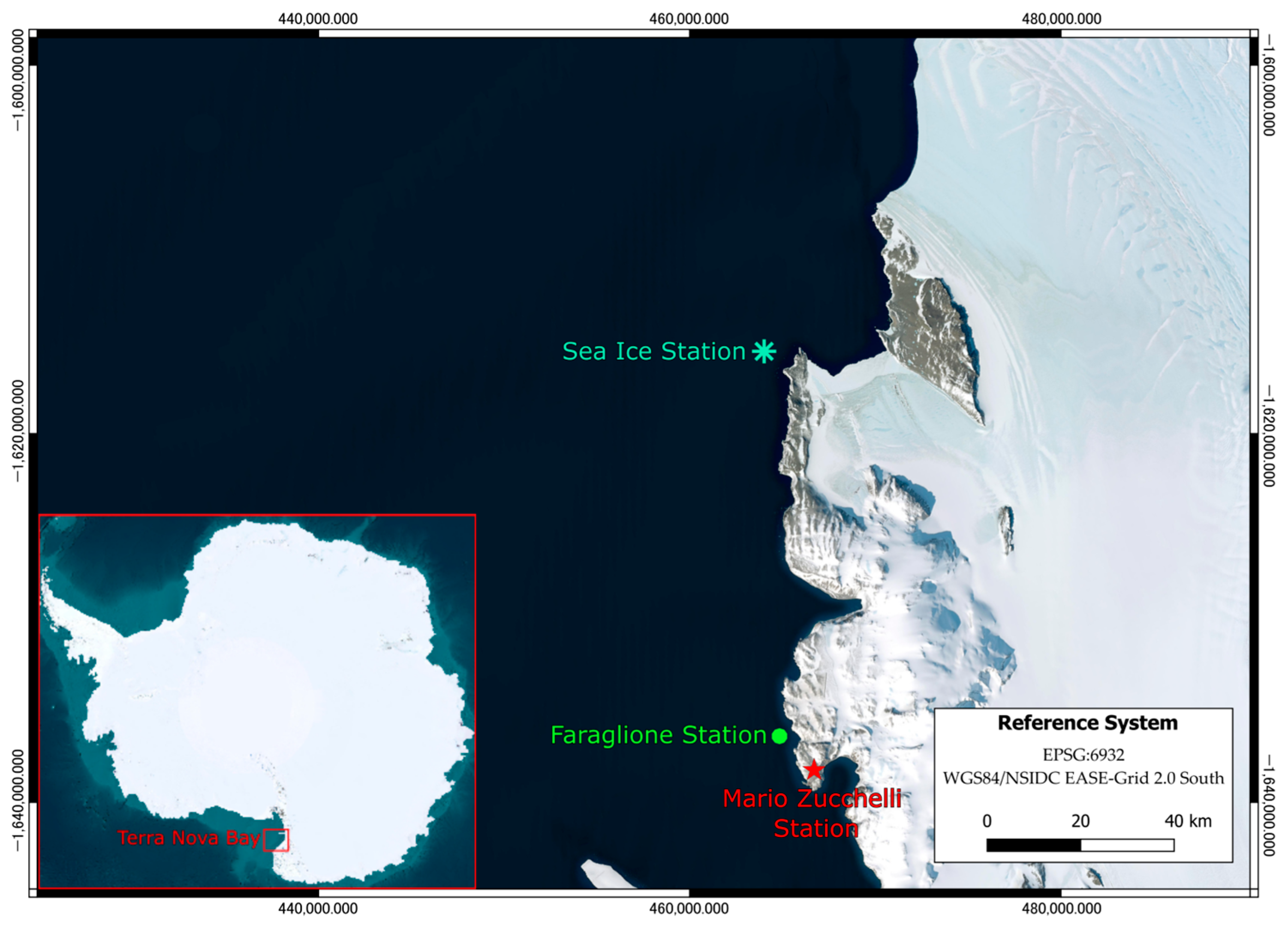
2.1. Study Area, Field and Laboratory Analysis

All the data in this study were detected at the Faraglione station (74°43′ S, 164°6′ E), close to the Mario Zucchelli research station corresponding to the 90 m depth bathymetry (Figure 1). Here, during 12 different PNRA campaigns (PNRA Expeditions 99-00, 00-01, 01-02, 02-03, 04-05, 09-10, 10-11, 11-12, 12-13, 14-15, 21-22, 22-23), 44 samplings were performed and bio-physical data were collected. Zooplankton was collected with vertical hauls from the bottom to the surface using a Bongo net or WP2 with a 200 μm mesh depending on the years.

Phytoplankton biomass was estimated by using fluorometers, validated with chlorophyll-a spectrofluorometric analyses or through HLPC methods in seawater samples (0.5-3L) drawn from the Niskin bottle at different sampling depths and filtrated on GFF filters [28,29], while environmental parameters such as salinity and temperature were obtained by CTD profiles using the Sea Bird 19 and the Idronaut 304 or 310 probes, depending on the years.

All zooplankton samples were preserved in a 4% buffered formaldehyde-seawater solution, except in the PNRA Expeditions 21-22 and 22-23, where the samples were preserved with 70% ethyl alcohol. Zooplankton taxonomic identification and counts were conducted using a stereomicroscope (Zeiss, Sydney, Australia). All samples were split with a Folsom plankton splitter into subsamples according to their abundance and were sorted into different taxa to the group level, while for copepods, an aliquot of the whole samples was considered, where at least 100 copepods could be identified at the species or genus level and life stage [30]. Zooplankton density was determined by dividing the total number of individuals by the volume of filtered water, expressed as individuals per cubic meter (m³).

For the trophic analysis of the mesozooplankton community, abundance has been converted into biomass by means of the proper weight/individual factors [31,32,33,34,35,36,37,38,39,40] reported in Table S1.

The conversion procedure has been validated by comparing the total biomass measured in the laboratory (dry weight method) [41] with the total biomass resulting from the conversion.

2.2. Data Processing

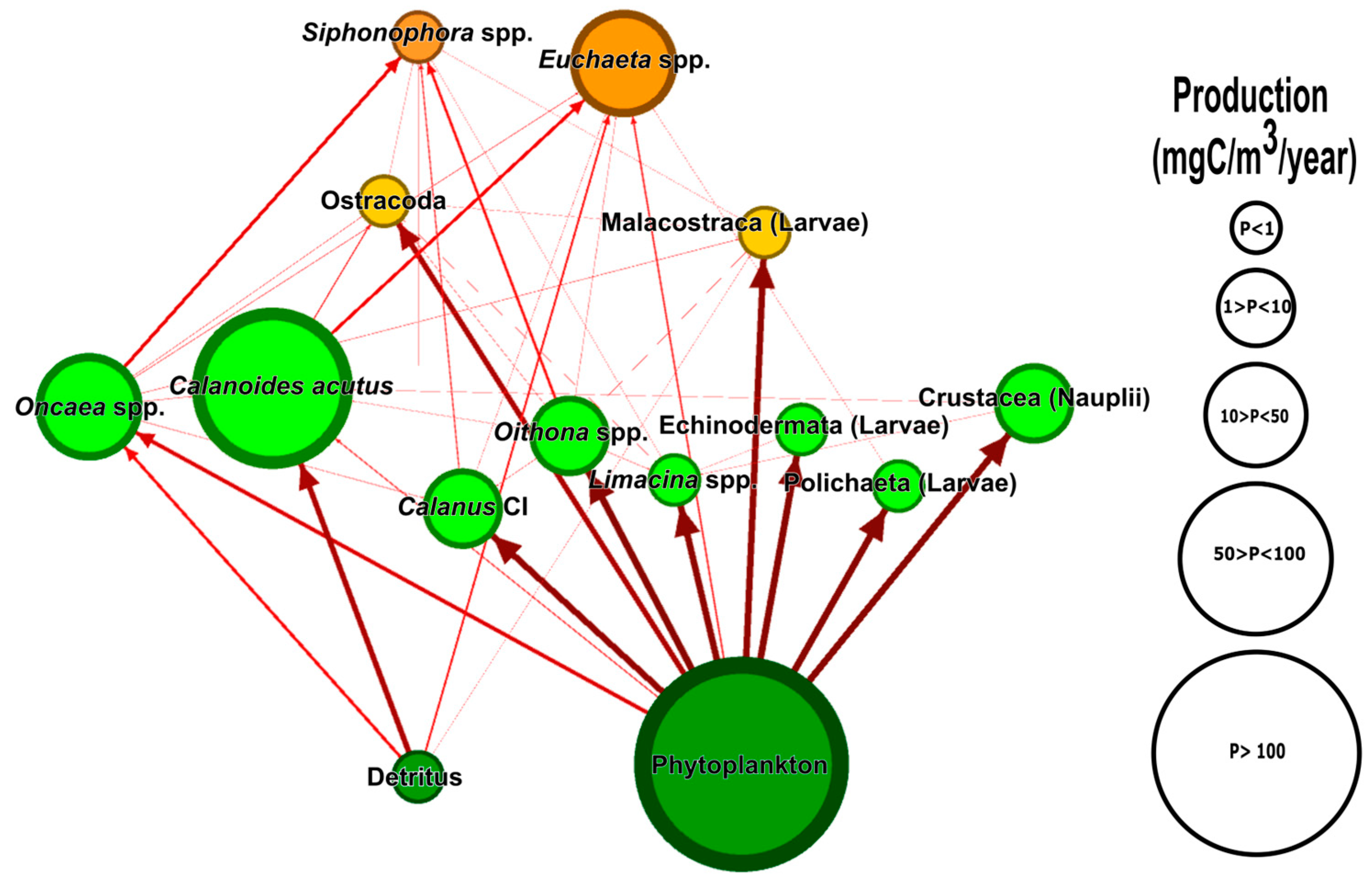
2.2.1. Mass Balanced Models

To characterize the structure and functioning of the mesozooplanktonic system, the model is based on the analysis and quantification of fluxes through different compartments [42,43,44]. The system flow analysis of the trophic network is based on the Ecopath with Ecosim (EwE) approach [27]. Ecopath is the foundational component of the EwE modeling suite, and it provides a static, mass-balanced snapshot of an ecosystem at a given point in time. Ecopath models divide the ecosystem into functional groups. These can be species, groups of species or life stages sharing similar ecological roles. The list of species considered in this study, together with their recognition as functional groups, generally based on the ecological role played by the species in the system, is reported in Table S1. This model requires several key parameters for each functional group: the biomass (B), consumption/biomass ratio (Q/B), production/biomass ratio (P/B), ecotrophic efficiency (EE) and diet matrix (DC). The parameters employed in this study are reported in Table S1. The diet matrix, balanced on the production of functional groups [45], is calculated starting from an adjacency matrix (Table S2), which represents the interactions between functional groups. In this study, the diet matrix was generated using the MATBLD method [46]. This method identifies predation pathways through the adjacency matrix, with diet fluxes allocated based on the combined proportion of predator demand and prey availability. Unlike the traditional binary adjacency matrix, this matrix uses integer values ranging from 3 (higher feeding preferences) to 0 (no interactions) to denote the varying preferences of predators for different prey groups.

The Ecopath approach grants that if one of these parameters is not entered, the missing one can be calculated, except for the diet matrix, which must always be present. Since ecotrophic efficiency is a parameter that is generally poorly known, it was always calculated in this study.

This methodology facilitated the derivation of numerous ecological indicators, which were subsequently used to assess the structure and functionality of the ecosystem.

2.2.2. Ecological Indicators

Using the Ecopath approach, different ecological indicators are obtained for the characterization of the structure and the functioning of the planktonic community [34,47,48].

Once the web of interaction in the community has been assessed, it is possible to assign to each functional group its specific trophic level, based on its role in the system.

The trophic level (TL) of each functional group was determined following the method of [49]. By convention, a TL of 1 is assigned to primary producers and detritus, while the TLs of other functional groups are calculated as follows:

$$\mathrm{T}{\mathrm{L}}_{\mathrm{j}}=1+{\displaystyle \sum _{\mathrm{i}=1}^{\mathrm{n}}}\mathrm{D}{\mathrm{C}}_{\mathrm{j}\mathrm{i}}\times \mathrm{T}{\mathrm{L}}_{\mathrm{i}}$$

where j is the predator of prey i, DC_ji is the fraction of prey i in the diet of predator j and TL_i is the trophic level of prey i. The mean trophic level of the system (MTL) is the arithmetic average of the trophic levels of all the functional groups in the system.

The Total System Throughput (TST) is defined as the summatory of all throughflows among all system compartments, using the following formula:

$$\mathrm{T}\mathrm{S}\mathrm{T}=\sum _{\mathrm{i}=1,\mathrm{j}=1}^{\mathrm{n}}{\mathrm{T}}_{\mathrm{i}\mathrm{j}}$$

where T_ij is the flux out of the i-group going in the j-group.

TST is considered a measure of system activity and is expected to grow during the development stages of the ecosystem, being related to system maturity [50].

While TST represents the quantity of energy moved in the system per unit of time, the efficiency of the energy exchanges in the system is identified by its average mutual information (AMI). A system composed of several compartments, with an equiprobability that a quantum of energy flows in several ways, has very low levels of information. But the reduction in the uncertainty (for a different, more organized distribution of the energy flows) makes the information obtained greater. The AMI is calculated as follows:

$$\mathrm{A}\mathrm{M}\mathrm{I}=\mathrm{K}\times \sum _{\mathrm{i},\mathrm{j}}\left({\displaystyle \frac{{\mathrm{T}}_{\mathrm{i}\mathrm{j}}}{\mathrm{T}\mathrm{S}\mathrm{T}}}\right)\times \mathrm{l}\mathrm{o}\mathrm{g}\left({\displaystyle \frac{{\mathrm{T}}_{\mathrm{i}\mathrm{j}}\times \mathrm{T}\mathrm{S}\mathrm{T}}{{\mathrm{T}}_{\mathrm{i}}\times {\mathrm{T}}_{\mathrm{j}}}}\right)$$

where T_ij is the flow from compartment i to compartment j, TST is the total system throughput and K is a scalar constant. Knowing the value and the direction of each output from the compartments in the system, it is possible to calculate the AMI of the system [51,52]. The result is a dimensionless value that is always greater than 0. The 0 is a value that would theoretically represent equiprobability in the direction of all flows and, consequently, the lowest value of organization and information in the system. The greater the flow, the better the organization of flows in the system [53].

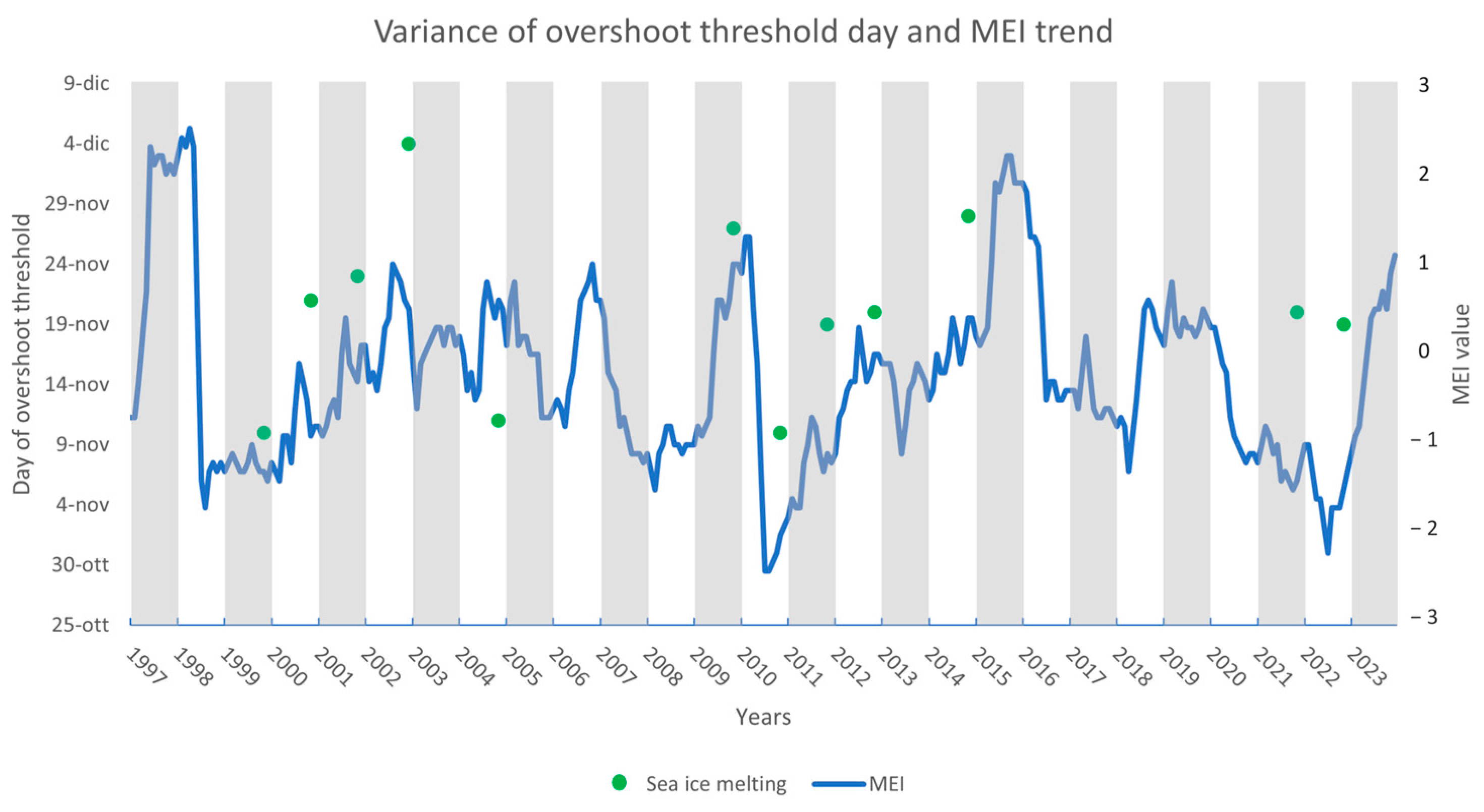
2.2.3. Days since Sea Ice Melting (DaSIM)

Aiming at the identification of the plankton community dynamics during the austral summer, it is crucial to determine when sea ice melting starts and, consequently, the trigger effect on primary producers due to sea ice algae released to the sea. Data reporting the sea ice concentration in Terra Nova Bay were obtained from the Copernicus dataset “Sea ice concentration daily gridded data from 1978 to present derived from satellite observations” (74°54′ S, 164°00′ E), referred to as Sea Ice Station in Figure 1 [54].

The moment of sea ice melting has been identified by testing several different hypotheses, specifically considering the moment when the sea ice concentration goes below 70% and maintains this condition for at least five consecutive days.

Once, per year, the moment when the sea ice coverage breaks is identified, we calculate a temporal distance from the sea ice melting to the sampling date.

For the sake of clarity, the austral summer is subdivided in four main phases as follows:

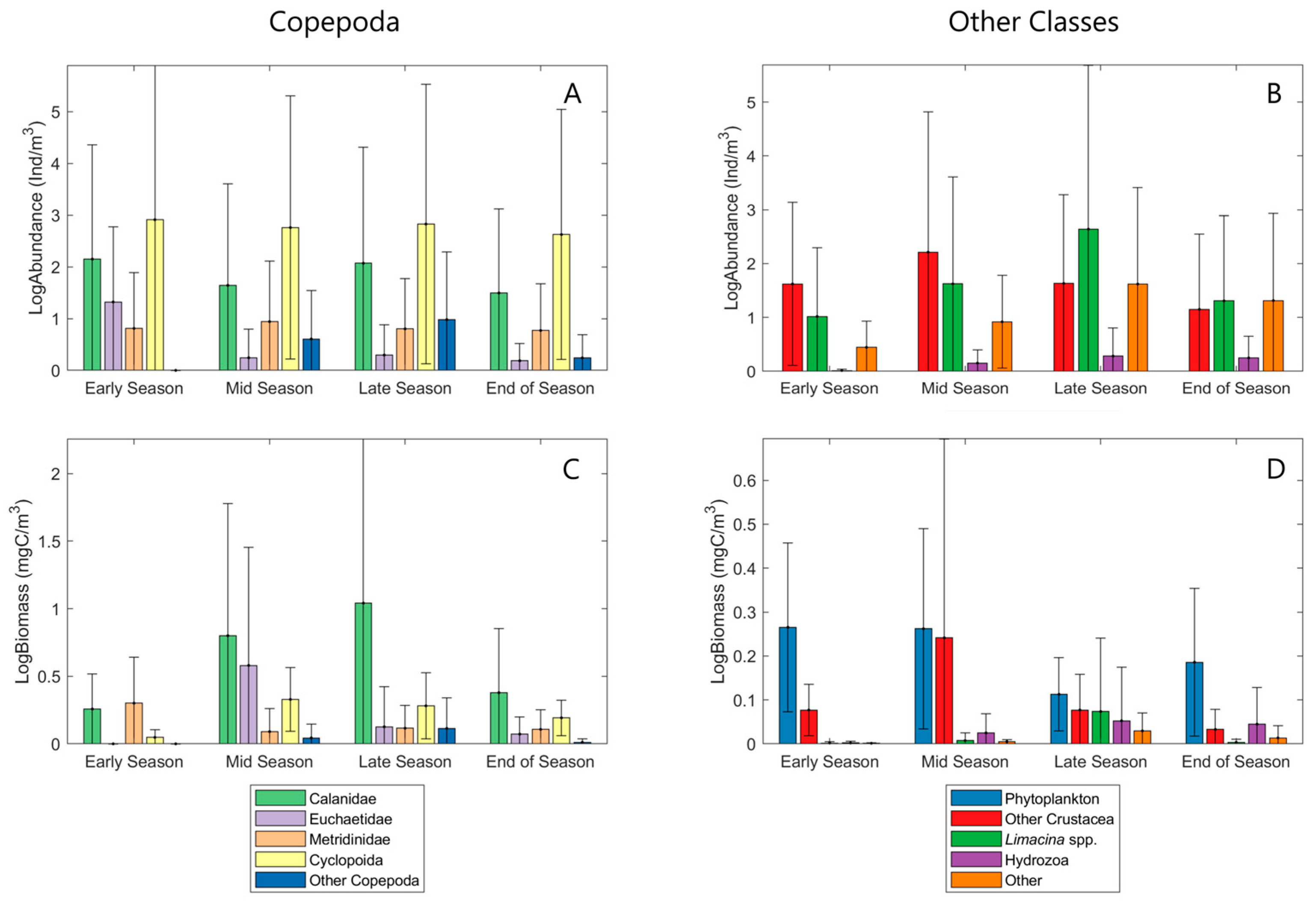
• Early Season: This is the initial phase of a season, characterized by the transition from the previous season. Weather patterns and environmental conditions begin to shift. For example, temperatures start to rise, ice coverage gets lower and the inner production is high due to solar radiation reaching the water body.
• Mid-Season: This stage marks the full development of the season’s typical characteristics. It represents the peak conditions of the season. For example, mid-summer is characterized by the hottest temperatures and longest days, and ice coverage is at a minimum.
• Late Season: This stage represents the gradual winding down of the season. The defining characteristics of the season start to weaken, and signs of the upcoming season begin to emerge. In late summer, for instance, temperatures warm up further while primary production is expected to decrease.
• End of Season: The final phase where the conditions transition into the next season. By the end of the summer, most of its distinct traits have faded. For instance, cooler temperatures signal the onset of fall.

2.2.4. Statistical Analyses

The MATrix LABoratory (MATLAB, ver 23.2) computer program’s “anova1” and “multcompare” functions were used to determine if statistically significant differences during austral summer were present between any of the four phases (Early season, Mid-season, Late season, End of season). The “anova1” function assumes all sample populations are normally distributed. One-way analysis of variance was conducted to test the null hypothesis that ecological indicators in different phases of the season have equal averages. If the null hypothesis is rejected (i.e., p < 0.01), a multiple comparison post hoc test using Tukey’s procedure was carried out to identify which phase is statistically different from the others (multcompare function) [55].

The relationship between the considered ecological indicators and several predictive variables (i.e., DaSIM, temperature, salinity) was tested by means of Generalized Additive Models (GAM) [56,57], aiming to assess what predictive variable is relevant to drive the ecology of the system.

3. Results

The list of functional groups and related biomasses of the 44 simulations analyzed are reported in Table S1.

Upon balancing the network of trophic interactions (an example given in Figure 2), the Ecopath approach was employed.

Figure 3 illustrates the day when sea ice coverage dropped below a specific threshold during the years of active sampling in Antarctica, alongside the dynamics of the Multivariate ENSO Index (MEI). Sea ice melting is generally delayed when the MEI is higher, but the two parameters are not significantly correlated (n = 12, r = 0.242, p > 0.1). The timing of sea ice melting, considered the starting point of the austral summer, exhibited a range of 24 days between the earliest and latest occurrences.

The structural and functional parameters of the mesozooplanktonic community were analyzed by means of Generalized Additive Models (GAM) in relation to several environmental parameters such as the sea temperature, salinity and DaSIM (

Table 1. Statistical significance of environmental parameters assessed through GAM (p-value).

	DaSIM	Temperature	Salinity
Total Biomass	<0.001	0.067
Primary Production	<0.001
Mean Trophic Level	0.002		0.006
Total system throughput	0.010
Average mutual information	0.003	0.049	0.033

). DaSIM resulted in the most significant parameters for explaining the dynamics of the considered community.

Ecological indicators were thus analyzed in relation to the time elapsed since the onset of sea ice melting. In Figure 4, the temporal range of the different phases of the austral summer considered in this study is shown.

The dynamics of the structure of the plankton community are reported in terms of abundance and biomass in (Figure 5–Table S3). The community is dominated both in terms of abundance and biomass by Copepods. This is why copepods are presented considering five different classifications. Specifically, Calanoida are subdivided into three families (Calanidae, Euchaetidae and Metridinidae), and Oithona spp. and Oncaea spp. are aggregated as Cyclopoida and, finally, other Copepoda. In terms of abundance, the community displays a certain stability during austral summer, with a sudden decrease in Euchaetidae mirrored by an increase in other copepods in the community and a low abundance of other groups during the end-of-season phase. The overall biomass trend shows higher values during the mid-season and late season mainly because of the dynamic of the Calanidae, which are, in terms of biomass, the most important group during the austral summer. On the contrary, Euchaeidae biomasses decrease starting from the late season, while Cyclopoida maintain their biomass at a stable level during the entire season. Considering other groups, it is worth noticing that the late season displayed the most balanced distribution of biomasses between the classes, also considering phytoplankton, which are at their seasonal minimum here.

Primary productivity (Figure 6A) decreases continuously until the late season and finally displays increasing values during the final phase of the austral summer (one-way ANOVA p < 0.01). An opposite trend is shown by MTL, resulting in a negative correlation with primary productivity (n = 44, r = −0.257, p < 0.1). MTL reaches its maximum values during the late season (Figure 6B). From a functional perspective, the overall activity of the community, represented by TST, follows the biomass trend, with slightly higher values during the intermediate phases of the season (Figure 6C). Finally, the organization level of flux exchanges within the system, represented by the Average Mutual Information (AMI), exhibits a similar trend as MTL (n = 44, r = 0.489, p < 0.01) (Figure 6D). Initially, AMI shows a sudden increase (one-way ANOVA p < 0.01), which continues until the late season, corresponding both to the peak in biomass and MTL (Figure 6B,D). Following this peak, the organization of flow exchanges decreases rapidly at the end of the season.

4. Discussion

This study aimed to investigate the evolution of the planktonic system communities in Terra Nova Bay during the austral summer. However, the Antarctic region, and especially the polynya zone, experiences significant year-to-year variability. In a system driven by sea ice cover, where organisms have very short development times, increasing the sampling effort is crucial to enhancing our understanding of this ephemeral habitat. Variations in sea ice concentration can result from global climate phenomena or natural fluctuations [58,59]. The onset of the austral summer is influenced by both local and general climatic conditions. General climatic conditions are depicted in Figure 3 through the variations in the Multivariate ENSO Index (MEI), which indicate the presence and intensity of the El Niño Southern Oscillation (ENSO) [60,61]. An MEI value above 0.5 indicates a moderate El Niño phenomenon, while a value above 1.2 indicates a strong El Niño phenomenon. Similarly, negative MEI values signify the La Niña phenomenon, with increasing intensity as the value decreases. Teleconnections’ effects on Antarctic sea ice have been studied and shown to be periodic or related to past events. Nevertheless, clear links between these phenomena and sea ice have yet to be established [62], but likely due to local specific conditions driven by factors operating on a smaller spatial scale. For example, the dynamics of mega icebergs are known to modify the Ross Sea circulation and productivity [63,64,65,66,67,68].

The Days since Sea Ice Melting (DaSIM) is a crucial result for the TNB study, as Figure 3 confirms. Over the twelve-year study period, the gap between the earliest and the latest moment of sea ice breaking is 24 days. In the short span of the austral summer, particularly during the sampling period, 24 days variation is significant, given the rapid development of the Antarctic environment. This is particularly important for studying the dynamics of organisms that develop rapidly under favorable conditions, as is the case in this study.

In TNB, the seasonal sea ice breaking proceeds from South to North [7,69], so Faraglione station should be reached by the melting later than Sea Ice Station, because this is quite distant from the sampling station. However, this delay can be assumed to remain fairly coherent throughout the years. Indeed, thanks to the DaSIM, our study’s results showed greater reliability, as it allows for observing the development of the system considering its triggering moment.

Examining the structure and functionality of ecological indicators allowed us to study the system’s evolution during the austral summer.

The entire mesozooplanktonic community is composed of 39 functional groups, but, including juvenile stages and the system subjected to a rapid evolution during summer, the community simulated was generally composed of an average number of 14 functional groups able to maintain a trophic web sustaining three trophic levels, as displayed in Figure 2. Despite the turnover of the functional groups in the web, few elements constantly characterize the composition of the system, being present in at least 90% of the samplings (namely, Calanoides acutus adult female, Oithona spp., Oncaea spp. and Polychaeta (Larvae)).

The systems start their summer activity with low biomass values rapidly increasing and reaching their peak later in the summer (late season), likely stimulated by the early phytoplankton bloom and the increased primary production activated by the higher solar radiation and nutrient availability triggered by the sea ice melting. The peak of primary production during the early season and mid-season copes well with the biomass increase later in the summer, indicating the development of the grazing system following the algal bloom.

Later in the season (End of season), a second (minor) phytoplanktonic bloom is likely to be recorded, confirming what is generally reported in literature [24,70,71,72], but this is not mirrored by any reaction in the mesozooplankton community biomass. This might be related to the late reaction already noted at the beginning of the season or to the presence of other players in the system not considered in this study, such as microzooplankton or the microbial community. Given model limitations in observing unaccounted compartments may explain the missed reaction of the observed system to the secondary peak of primary production, which is likely to be addressed to other functional groups not considered here [57,58].

The functioning of the system follows the biomass and productivity trend displaying a change in the trophic web organization well represented by the MTL dynamics. Once the primary productivity released new organic matter in the system, the available resources were exploited and moved up toward a higher trophic level, increasing the biomass and activity of secondary consumers such as Euchaetidae and other crustacea during the mid-season.

This change in the system organization is not mirrored by significant changes in the overall system activity (TST), but it is recorded by the efficiency of flow exchange in the system (AMI). The system, in fact, became more efficient during intermediate phases of the season, when production was lower but the energy balance of the system was high due to its complexity. As a reaction, the planktonic community moves towards more efficient relationships to maximize the available energy once internal production is lower [69,73,74,75,76].

5. Conclusions

It is therefore possible to summarize the dynamics of the coastal mesozooplanktonic community of Terra Nova Bay as follows. The system is capable of rapidly exploiting the possibilities given by the summer season onset displaying the first phase of intense development. The primary productivity of the system rises with a phytoplanktonic bloom well established in the mid-season, supporting a significant biomass increase. The biomass stabilizes thanks to the development of the grazing system, as highlighted by the AMI trend. During the late season, the ecological indicators suggest the development of a different stage of the system that it is likely preparing for the autumn phase composed of species capable of facing harsh environmental conditions due to a thick ice cover. Here, the system displays maximum organization together with a shift towards consumption over production (maximum MTL). However, the primary production shows a rebound effect, with a second peak in the last phases of the austral summer, referable to a second phytoplankton bloom, probably due to different primary producers that are not easily accessible by the mesozooplankton community. For this reason, neither the biomass nor the efficiency of the considered system show an increase, suggesting that this phytoplanktonic bloom is likely to be exploited by other communities.

In conclusion, the mesozooplankton network in Terra Nova Bay’s coastal area emerges as a dynamically evolving system. Throughout this study, standardizing data to a consistent austral summer starting point, by means of a DaSIM indicator, proved to be essential for the sake of developing a diachronic analysis of the mesozooplankton community in Terra Nova Bay. While modeling approaches like the one proposed here effectively capture system dynamics, enhanced sampling and organizational efforts are imperative for deeper insights into compartmental evolution during the austral summer and for developing theories that accommodate inter-annual variations, also considering Antarctica’s critical vulnerability to climate change impacts.

References

1. Deppeler, S.L.; Davidson, A.T. Southern Ocean Phytoplankton in a Changing Climate. Front. Mar. Sci. 2017, 4, 40. [Google Scholar] [CrossRef]
2. Catalano, G.; Povero, P.; Fabiano, M.; Benedetti, F.; Goffart, A. Nutrient Utilisation and Particulate Organic Matter Changes during Summer in the Upper Mixed Layer (Ross Sea, Antarctica). Deep Sea Res. Part I Oceanogr. Res. Pap. 1997, 44, 97–112. [Google Scholar] [CrossRef]
3. Smith, W.O.; Nelson, D.M. Phytoplankton Bloom Produced by a Receding Ice Edge in the Ross Sea: Spatial Coherence with the Density Field. Science 1985, 227, 163–166. [Google Scholar] [CrossRef] [PubMed]
4. Kasyan, V.V. Recent Changes in Composition and Distribution Patterns of Summer Mesozooplankton off the Western Antarctic Peninsula. Water 2023, 15, 1948. [Google Scholar] [CrossRef]
5. Johnston, N.M.; Murphy, E.J.; Atkinson, A.; Constable, A.J.; Cotté, C.; Cox, M.; Daly, K.L.; Driscoll, R.; Flores, H.; Halfter, S.; et al. Status, Change, and Futures of Zooplankton in the Southern Ocean. Front. Ecol. Evol. 2022, 9, 624692. [Google Scholar] [CrossRef]
6. Stevens, C.J.; Pakhomov, E.A.; Robinson, K.V.; Hall, J.A. Mesozooplankton Biomass, Abundance and Community Composition in the Ross Sea and the Pacific Sector of the Southern Ocean. Polar Biol. 2015, 38, 275–286. [Google Scholar] [CrossRef]
7. Lin, Y.; Yang, Q.; Mazloeff, M.; Wu, X.; Tian-Kunze, X.; Kaleschke, L.; Yu, L.; Chen, D. Transiting Consolidated Ice Strongly Influenced Polynya Area during a Shrink Event in Terra Nova Bay in 2013. Commun. Earth Environ. 2023, 4, 54. [Google Scholar] [CrossRef]
8. Jendersie, S.; Williams, M.J.M.; Langhorne, P.J.; Robertson, R. The Density-Driven Winter Intensification of the Ross Sea Circulation. J. Geophys. Res. Oceans 2018, 123, 7702–7724. [Google Scholar] [CrossRef]
9. Orsi, A.H.; Wiederwohl, C.L. A Recount of Ross Sea Waters. Deep Sea Res. II Top. Stud. Oceanogr. 2009, 56, 778–795. [Google Scholar] [CrossRef]
10. Miller, U.K.; Zappa, C.J.; Gordon, A.L.; Yoon, S.T.; Stevens, C.; Lee, W.S. High Salinity Shelf Water Production Rates in Terra Nova Bay, Ross Sea from High-Resolution Salinity Observations. Nat. Commun. 2024, 15, 373. [Google Scholar] [CrossRef]
11. Semprucci, F.; Appolloni, L.; Grassi, E.; Donnarumma, L.; Cesaroni, L.; Tirimberio, G.; Chianese, E.; Di Donato, P.; Russo, G.F.; Balsamo, M.; et al. Antarctic Special Protected Area 161 as a Reference to Assess the Effects of Anthropogenic and Natural Impacts on Meiobenthic Assemblages. Diversity 2021, 13, 626. [Google Scholar] [CrossRef]
12. Pane, L.; Feletti, M.; Francomacaro, B.; Mariottini, G.L. Summer Coastal Zooplankton Biomass and Copepod Community Structure near the Italian Terra Nova Base (Terra Nova Bay, Ross Sea, Antarctica). J. Plankton Res. 2004, 26, 1479–1488. [Google Scholar] [CrossRef]
13. Sertorio, T.Z.; Licandro, P.; Ossola, C.; Artegiani, A. Copepod Communities in the Pacific Sector of the Southern Ocean in Early Summer. In Ross Sea Ecology; Springer: Berlin/Heidelberg, Germany, 2000; pp. 291–307. [Google Scholar]
14. Povero, P.; Chiantore, M.; Misic, C.; Budillon, G.; Cattaneo-Vietti, R. Land Forcing Controls Pelagic-Benthic Coupling in Adelie Cove (Terra Nova Bay, Ross Sea). Polar Biol. 2001, 24, 875–882. [Google Scholar] [CrossRef]
15. Povero, P.; Castellano, M.; Ruggieri, N.; Monticelli, L.S.; Saggiomo, V.; Chiantore, M.; Guidetti, M.; Cattaneo-Vietti, R. Water Column Features and Their Relationship with Sediments and Benthic Communities along the Victoria Land Coast, Ross Sea, Summer 2004. Antarct. Sci. 2006, 18, 603–613. [Google Scholar] [CrossRef]
16. Minutoli, R.; Bonanno, A.; Guglielmo, L.; Bergamasco, A.; Grillo, M.; Schiaparelli, S.; Barra, M.; Bergamasco, A.; Remirens, A.; Genovese, S.; et al. Biodiversity and Functioning of Mesozooplankton in a Changing Ross Sea. Deep Sea Res. Part II Top. Stud. Oceanogr. 2024, 217, 105401. [Google Scholar] [CrossRef]
17. LTER Italy—MBT-IT17-005-M. Available online: https://deims.org/7fb8e2c6-b11f-41a7-b494-44ceeb3bed2d (accessed on 26 July 2024).
18. Arrigo, K.R.; McClain, C.R. Spring Phytoplankton Production in the Western Ross Sea. Science 1994, 266, 261–263. [Google Scholar] [CrossRef]
19. Smith, W.O.; Gordon, L.I. Hyperproductivity of the Ross Sea (Antarctica) Polynya during Austral Spring. Geophys. Res. Lett. 1997, 24, 233–236. [Google Scholar] [CrossRef]
20. Mangoni, O.; Saggiomo, M.; Bolinesi, F.; Castellano, M.; Povero, P.; Saggiomo, V.; DiTullio, G.R. Phaeocystis Antarctica Unusual Summer Bloom in Stratified Antarctic Coastal Waters (Terra Nova Bay, Ross Sea). Mar. Environ. Res. 2019, 151, 104733. [Google Scholar] [CrossRef]
21. Nuccio, C.; Innamorati, M.; Lazzara, L.; Mori, G.; Massi, L. Spatial and Temporal Distribution of Phytoplankton Assemblages in the Ross Sea. In Ross Sea Ecology, Italian Antarctic Expeditions (1987–1995); Faranda, F.M., Guglielmo, L., Ianora, A., Eds.; Springer: Berlin/Heidelberg, Germany, 2000; pp. 231–245. [Google Scholar]
22. Smith, W.O.; Ainley, D.G.; Arrigo, K.R.; Dinniman, M.S. The Oceanography and Ecology of the Ross Sea. Ann. Rev. Mar. Sci. 2014, 6, 469–487. [Google Scholar] [CrossRef]
23. Mangoni, O.; Saggiomo, V.; Bolinesi, F.; Margiotta, F.; Budillon, G.; Cotroneo, Y.; Misic, C.; Rivaro, P.; Saggiomo, M. Phytoplankton Blooms during Austral Summer in the Ross Sea, Antarctica: Driving Factors and Trophic Implications. PLoS ONE 2017, 12, e0176033. [Google Scholar] [CrossRef]
24. Knox, G.A. The Biology of the Southern Ocean; Cambridge University Press: Cambridge, UK, 1994. [Google Scholar]
25. Hopkins, T.L.; Torres, J.J. Midwater Food Web in the Vicinity of a Marginal Ice Zone in the Western Weddell Sea. Deep Sea Res. Part A Oceanogr. Res. Pap. 1989, 36, 543–560. [Google Scholar] [CrossRef]
26. Carli, A.; Pane, L.; Stocchino, C. Planktonic Copepods in Terra Nova Bay (Ross Sea): Distribution and Relationship with Environmental Factors. In Ross Sea Ecology; Springer: Berlin/Heidelberg, Germany, 2000. [Google Scholar]
27. Christensen, V. A Model of Trophic Interactions in the North Sea in 1981, the Year of the Stomach. Dana 2003, 11, 1–18. [Google Scholar]
28. Vidussi, F.; Claustre, H.; Bustillos-Guzmàn, J.; Cailliau, C.; Marty, J.C. Determination of Chlorophylls and Carotenoids of Marine Phytoplankton: Separation of Chlorophyll a from Divinylchlorophyll a and Zeaxanthin from Lutein. J. Plankton Res. 1996, 18, 2377–2382. [Google Scholar] [CrossRef]
29. Holm-Hansen, O.; Lorenzen, C.J.; Holmes, R.W.; Strickland, J.D.H. Fluorometric Determination of Chlorophyll. ICES J. Mar. Sci. 1965, 30, 3–15. [Google Scholar] [CrossRef]
30. Frontier, S. Calcul de l’erreur Sur Un Comptage de Zooplancton. J. Exp. Mar. Biol. Ecol. 1972, 8, 121–132. [Google Scholar] [CrossRef]
31. Hunt, B.P.V.; Pakhomov, E.A.; Hosie, G.W.; Siegel, V.; Ward, P.; Bernard, K. Pteropods in Southern Ocean Ecosystems. Prog. Oceanogr. 2008, 78, 193–221. [Google Scholar] [CrossRef]
32. Boysen-Ennen, E.; Hagen, W.; Hubold, G.; Piatkowski, U. Zooplankton Biomass in the Ice-Covered Weddell Sea, Antarctica. Mar. Biol. 1991, 111, 227–235. [Google Scholar] [CrossRef]
33. Schnack-Schiel, S.B.; Hagen, W.; Mizdalski, E. Seasonal Comparison of Calanoides Acutus and Calanus Propinquus (Copepoda: Calanoida) in the Southeastern Weddel Sea, Antarctica. Mar. Ecol. Prog. Ser. 1991, 70, 17–27. [Google Scholar] [CrossRef]
34. Vassallo, P.; Bellardini, D.; Castellano, M.; Dapueto, G.; Povero, P. Structure and Functionality of the Mesozooplankton Community in a Coastal Marine Environment: Portofino Marine Protected Area (Liguria). Diversity 2022, 14, 19. [Google Scholar] [CrossRef]
35. Bednaršek, N.; Mozina, J.; Vogt, M.; O’Brien, C.; Tarling, G.A. The Global Distribution of Pteropods and Their Contribution to Carbonate and Carbon Biomass in the Modern Ocean. Earth Syst. Sci. Data 2012, 4, 167–186. [Google Scholar] [CrossRef]
36. Bednaršek, N.; Tarling, G.A.; Fielding, S.; Bakker, D.C.E. Population Dynamics and Biogeochemical Significance of Limacina helicina Antarctica in the Scotia Sea (Southern Ocean). Deep Sea Res. II Top. Stud. Oceanogr. 2012, 59–60, 105–116. [Google Scholar] [CrossRef]
37. Pond, D.W.; Ward, P. Importance of Diatoms for Oithona in Antarctic Waters. J. Plankton Res. 2011, 33, 105–118. [Google Scholar] [CrossRef]
38. Garcia, M.D.; Hoffmeyer, M.S.; Abbate, M.C.L.; Barría de Cao, M.S.; Pettigrosso, R.E.; Almandoz, G.O.; Hernando, M.P.; Schloss, I.R. Micro- and Mesozooplankton Responses during Two Contrasting Summers in a Coastal Antarctic Environment. Polar Biol. 2016, 39, 123–137. [Google Scholar] [CrossRef]
39. Kerkar, A.U.; Venkataramana, V.; Tripathy, S.C. Assessing the Trophic Link between Primary and Secondary Producers in the Southern Ocean: A Carbon-Biomass Based Approach. Polar Sci. 2022, 31, 100734. [Google Scholar] [CrossRef]
40. Brey, T. Estimating Productivity of Macrobenthic Invertebrates from Biomass and Mean Individual Weight. Meeresforsch 1990, 32, 329–343. [Google Scholar]
41. Misic, C.; Bavestrello, G.; Bo, M.; Borghini, M.; Castellano, M.; Covazzi Harriague, A.; Massa, F.; Spotorno, F.; Povero, P. The “Seamount Effect” as Revealed by Organic Matter Dynamics around a Shallow Seamount in the Tyrrhenian Sea (Vercelli Seamount, Western Mediterranean). Deep Sea Res. Part I Oceanogr. Res. Pap. 2012, 67, 1–11. [Google Scholar] [CrossRef]
42. Paoli, C.; Morten, A.; Bianchi, C.N.; Morri, C.; Fabiano, M.; Vassallo, P. Capturing Ecological Complexity: OCI, a Novel Combination of Ecological Indices as Applied to Benthic Marine Habitats. Ecol. Indic. 2016, 66, 86–102. [Google Scholar] [CrossRef]
43. Vassallo, P.; Paoli, C.; Fabiano, M. Ecosystem Level Analysis of Sandy Beaches Using Thermodynamic and Network Analyses: A Study Case in the NW Mediterranean Sea. Ecol. Indic. 2012, 15, 10–17. [Google Scholar] [CrossRef]
44. Vassallo, P.; Paoli, C.; Schiavon, G.; Albertelli, G.; Fabiano, M. How Ecosystems Adapt to Face Disruptive Impact? The Case of a Commercial Harbor Benthic Community. Ecol. Indic. 2013, 24, 431–438. [Google Scholar] [CrossRef]
45. Heymans, J.J.; Coll, M.; Link, J.S.; Mackinson, S.; Steenbeek, J.; Walters, C.; Christensen, V. Best Practice in Ecopath with Ecosim Food-Web Models for Ecosystem-Based Management. Ecol. Model. 2016, 331, 173–184. [Google Scholar] [CrossRef]
46. Ulanowicz, R.E.; Scharler, U.M. Least-Inference Methods for Constructing Networks of Trophic Flows. Ecol. Model. 2008, 210, 278–286. [Google Scholar] [CrossRef]
47. Vassallo, P.; D’Onghia, G.; Fabiano, M.; Maiorano, P.; Lionetti, A.; Paoli, C.; Sion, L.; Carlucci, R. A Trophic Model of the Benthopelagic Fauna Distributed in the Santa Maria Di Leuca Cold-Water Coral Province (Mediterranean Sea). Energy Ecol. Environ. 2017, 2, 114–124. [Google Scholar] [CrossRef]
48. Christensen, V.; Walters, C.J. Ecopath with Ecosim: Methods, Capabilities and Limitations. Ecol. Model. 2004, 172, 109–139. [Google Scholar] [CrossRef]
49. Odum, W.E.; Heald, E.J. The Detritus-Based Food Web of an Estuarine Mangrove Community. Estuar. Res. 1975, 1, 265–286. [Google Scholar]
50. Odum, E.P. The Strategy of Ecosystem Development. Science 1969, 164, 262–270. [Google Scholar] [CrossRef] [PubMed]
51. Ulanowicz, R.E. Growth and Development: Ecosystem Phenomenology; Springer: New York, NY, USA, 1986. [Google Scholar]
52. Scharler, U.M. Ecological Network Analysis, Ascendency. In Ecosystem Ecology; Jorgensen, S.E., Ed.; Elsevier B.V.: Amsterdam, The Netherlands, 2009; pp. 57–64. [Google Scholar]
53. Gilbert, A.J. Connectance Indicates the Robustness of Food Webs When Subjected to Species Loss. Ecol. Indic. 2009, 9, 72–80. [Google Scholar] [CrossRef]
54. Copernicus Climate Change Service (C3S) Climate Data Store (CDS). Copernicus Climate Change Service (C3S) (2024): Sea Ice Concentration Daily Gridded Data from 1979 to Present Derived from Satellite Observations. Available online: https://cds.climate.copernicus.eu/cdsapp#!/dataset/satellite-sea-ice-concentration?tab=form (accessed on 10 September 2024).
55. The MathWorks Inc. Optimization Toolbox, Version: R2023b (23.2.0.2428915); The MathWorks Inc.: Natick, MA, USA, 2022. [Google Scholar]
56. Hastie, T.; Tibshirani, R. Generalized Additive Models: Some Applications. J. Am. Stat. Assoc. 1987, 82, 371–386. [Google Scholar] [CrossRef]
57. Wood, S.N. Fast Stable Restricted Maximum Likelihood and Marginal Likelihood Estimation of Semiparametric Generalized Linear Models. J. R. Stat. Soc. Ser. B Stat. Methodol. 2011, 73, 3–36. [Google Scholar] [CrossRef]
58. Lecomte, O.; Goosse, H.; Fichefet, T.; De Lavergne, C.; Barthélemy, A.; Zunz, V. Vertical Ocean Heat Redistribution Sustaining Sea-Ice Concentration Trends in the Ross Sea. Nat. Commun. 2017, 8, 258. [Google Scholar] [CrossRef]
59. Arrigo, K.R.; Van Dijken, G.L. Annual Changes in Sea-Ice, Chlorophyll a, and Primary Production in the Ross Sea, Antarctica. Deep Sea Res. Part II Top. Stud. Oceanogr. 2004, 51, 117–138. [Google Scholar] [CrossRef]
60. Wolter, K.; Timlin, M.S. El Niño/Southern Oscillation Behaviour since 1871 as Diagnosed in an Extended Multivariate ENSO Index (MEI.Ext). Int. J. Climatol. 2011, 31, 1074–1087. [Google Scholar] [CrossRef]
61. NOAA Physical Sciences Laboratory. Available online: https://psl.noaa.gov/enso/mei/ (accessed on 25 July 2024).
62. Turner, J. The El Niño-Southern Oscillation and Antarctica. Int. J. Climatol. 2004, 24, 1–31. [Google Scholar] [CrossRef]
63. Robinson, N.J.; Williams, M.J.M. Iceberg-Induced Changes to Polynya Operation and Regional Oceanography in the Southern Ross Sea, Antarctica, from in Situ Observations. Antarct. Sci. 2012, 24, 514–526. [Google Scholar] [CrossRef]
64. Martin, S.; Drucker, R.S.; Kwok, R. The Areas and Ice Production of the Western and Central Ross Sea Polynyas, 1992–2002, and Their Relation to the B-15 and C-19 Iceberg Events of 2000 and 2002. J. Mar. Syst. 2007, 68, 201–214. [Google Scholar] [CrossRef]
65. Harangozo, S.A.; Connolley, W.M. The Role of the Atmospheric Circulation in the Record Minimum Extent of Open Water in the Ross Sea in the 2003 Austral Summer. Atmosphere-Ocean 2006, 44, 83–97. [Google Scholar] [CrossRef]
66. Brunt, K.M.; Sergienko, O.; MacAyeal, D.R. Observations of Unusual Fast-Ice Conditions in the Southwest Ross Sea, Antarctica: Preliminary Analysis of Iceberg and Storminess Effects. Ann. Glaciol. 2006, 44, 183–187. [Google Scholar] [CrossRef]
67. Arrigo, K.R.; van Dijken, G.L. Impact of Iceberg C-19 on Ross Sea Primary Production. Geophys. Res. Lett. 2003, 30, 1836. [Google Scholar] [CrossRef]
68. Smith, K.L. Free-Drifting Icebergs in the Southern Ocean: An Overview. Deep Sea Res. Part II Top. Stud. Oceanogr. 2011, 58, 1277–1284. [Google Scholar] [CrossRef]
69. Rossi, L.; Sporta Caputi, S.; Calizza, E.; Careddu, G.; Oliverio, M.; Schiaparelli, S.; Costantini, M.L. Antarctic Food Web Architecture under Varying Dynamics of Sea Ice Cover. Sci. Rep. 2019, 9, 12454. [Google Scholar] [CrossRef]
70. Saggiomo, V.; Carrada, G.C.; Mangoni, O.; D’alcalà, M.R.; Russo, A. Spatial and Temporal Variability of Size-Fractionated Biomass and Primary Production in the Ross Sea (Antarctica) during Austral Spring and Summer. J. Mar. Syst. 1998, 17, 115–127. [Google Scholar] [CrossRef]
71. Arrigo, K.R.; Weiss, A.M.; Smith, W.O. Physical Forcing of Phytoplankton Dynamics in the Southwestern Ross Sea. J. Geophys. Res. Oceans 1998, 103, 1007–1021. [Google Scholar] [CrossRef]
72. Saggiomo, M.; Escalera, L.; Bolinesi, F.; Rivaro, P.; Saggiomo, V.; Mangoni, O. Diatom Diversity during Two Austral Summers in the Ross Sea (Antarctica). Mar. Micropaleontol. 2021, 165, 101993. [Google Scholar] [CrossRef]
73. Cau, A.; Ennas, C.; Moccia, D.; Mangoni, O.; Bolinesi, F.; Saggiomo, M.; Granata, A.; Guglielmo, L.; Swadling, K.M.; Pusceddu, A. Particulate Organic Matter Release below Melting Sea Ice (Terra Nova Bay, Ross Sea, Antarctica): Possible Relationships with Zooplankton. J. Mar. Syst. 2021, 217, 103510. [Google Scholar] [CrossRef]
74. Granata, A.; Weldrick, C.K.; Bergamasco, A.; Saggiomo, M.; Grillo, M.; Bergamasco, A.; Swadling, K.M.; Guglielmo, L. Diversity in Zooplankton and Sympagic Biota during a Period of Rapid Sea Ice Change in Terra Nova Bay, Ross Sea, Antarctica. Diversity 2022, 14, 425. [Google Scholar] [CrossRef]
75. Monti-Birkenmeier, M.; Diociaiuti, T.; Bolinesi, F.; Saggiomo, M.; Mangoni, O. Microzooplankton and Phytoplankton of Ross Sea Polynya Areas and Potential Linkage among Functional Traits. Deep Sea Res. II Top. Stud. Oceanogr. 2024, 216, 105393. [Google Scholar] [CrossRef]
76. Monti, M.; Zoccarato, L.; Fonda Umani, S. Microzooplankton Composition under the Sea Ice and in the Open Waters in Terra Nova Bay (Antarctica). Polar Biol. 2017, 40, 891–901. [Google Scholar] [CrossRef]
Figure 1. In the lower left corner, there is an overview of Antarctica. In the image, Terra Nova Bay is shown. Red star: Mario Zucchelli Station, Green circle: Faraglione Station (sampling point), Blue Asterisk: Sea Ice Station (data from satellite).
Diversity 16 00600 g001
Figure 2. Example of a trophic network structure resulting from modelling approach. The dimension of nodes represents the production of functional group (mgC/m3/year) divided into five classes. The dimension and the color of arrows (from dark red to light red) represent the intensity of the flows.
Diversity 16 00600 g002
Figure 3. MEI values from 1997 to 2023 and, for the years covered in this study, the day when the ice coverage threshold was reached. The blue line represents the MEI trend, and the green marks the day when the ice coverage threshold was reached.
Diversity 16 00600 g003
Figure 4. Temporal range of summer season phases.
Diversity 16 00600 g004
Figure 5. Trend of abundances (individual/m3) and biomasses (mgC/m3) during the austral summer. Subplot (A): copepods’ abundances; Subplot (B): other classes’ abundances; Subplot (C): copepods’ biomasses; Subplot (D): other classes’ abundances.
Diversity 16 00600 g005
Figure 6. Ecological indicators trend during austral summer ((A): Net Primary production; (B): Mean trophic level; (C): Total system throughput; (D): Average mutual information). The line inside of each box is the sample median. The top and bottom edges of each box are the upper and lower quartiles, respectively. Vertical lines represent the distribution of data within 1.5 times the interquartile range, while circles are data out of this range (outliers).
Diversity 16 00600 g006