Elucidating the Disrupted Seasonal Cycle of Eodiaptomus japonicus (Calanoida, Copepoda) in Lake Biwa: Insights from an Individual-Based Model

Abstract

The seasonal fluctuations of the copepod Eodiaptomus japonicus, which dominates the zooplankton community of Lake Biwa, have been disrupted several times over the past 45 years. The aim of this study was to clarify the primary environmental factor that caused the disrupted seasonal cycle in population density of E. japonicus. Here, we tested the hypothesis that the disruption in their seasonal cycle was due to the impacts of water temperature, food conditions, and predator pressure, using an individual-based model (IBM). Based on the experimental data from the literature, we described the growth and reproduction of E. japonicus using temperature- and food-dependent functions. Previously, the developmental time of this species was expressed using Bělehrádek’s equation. In this study, we applied the Kontodimas equation, which successfully reproduced the effects of food scarcity at higher temperatures. Additionally, the influence of predators was incorporated into the survival rate of adult individuals. The long-term data set of Lake Biwa was input into the developed model to simulate the population fluctuations during the disruption period (1975–1979) and stable period (1995–1999) of their seasonal cycle. The combination of environmental data to be input was (1) water temperature, food availability, and predators; (2) water temperature and food availability; and (3) water temperature and predators. Disruptions in the seasonal cycle of the population were only observed in scenario (1) during the disruption period simulation, suggesting that the disrupted seasonal cycle of this species in Lake Biwa may have been caused by the effects of both food condition and predators. The results of simulation scenarios (2) and (3) indicated that predators have a stronger impact on the population than food availability. This time, we used common and simple indicators to describe food conditions and predators, but the model can be improved to be more complex and accurate as more data become available. Such models are important tools for understanding the relationship between environmental factors and the dynamics of diaptomid copepod populations.

1. Introduction

Lake ecosystems, being sensitive entities, undergo significant transformations that extend beyond natural factors. Among the inhabitants of these ecosystems, zooplankton populations stand out as particularly vulnerable to the multifaceted impacts of environmental changes due to their limited ability to migrate over extensive distances in search of optimal conditions. The primary response of lacustrine zooplankton to climate-induced change is a shift in seasonality, a response that resonates throughout the entire community and holds the potential to alter the intricate structure of the food web [1,2].

Lake Biwa, the largest and oldest lake in Japan, stands as a testament to its extensive history and diverse ecological landscape. Renowned for its rich biodiversity, the lake is home to over 60 endemic species. Beyond its ecological significance, Lake Biwa plays a pivotal role in supporting the livelihoods of approximately 15 million people in the surrounding prefectures, serving as a vital water source and contributing significantly to the development of fisheries and agriculture [3]. However, over the past six decades, Lake Biwa has faced the repercussions of anthropogenic activities. The rapid economic growth of the 1950s triggered an upsurge in water pollution and eutrophication, with synthetic detergents and phosphates identified as key contributors to these environmental challenges [4,5,6]. A plan to reduce nitrogen and phosphorus input from effluent into the lake was implemented after 1980. Subsequently, both nitrogen and phosphorus loadings from the watershed of Lake Biwa gradually decreased after the 1980s [7]. However, since the late 1980s, the surface temperature of the lake has increased by 1 °C, likely due to global warming [8]. Additionally, fisheries catch data have revealed a decrease in planktivorous fishes since 1990 [9]. Against this backdrop, understanding the dynamics of dominant copepod populations in Lake Biwa becomes imperative, as these organisms play a pivotal role in navigating the delicate equilibrium of this ecosystem amidst both natural and anthropogenic challenges.

The calanoid copepod Eodiaptomus japonicus emerges as a central figure within the intricate dynamics of Lake Biwa’s zooplankton community. Over the course of more than five decades, E. japonicus has steadfastly dominated, constituting 70% of the total biomass [10]. Beyond its sheer abundance, this copepod assumes a critical role as an important food resource for planktivorous fish [11], thereby exerting a profound influence on the lake’s food web. In light of its ecological significance, numerous studies have delved into the various facets of E. japonicus [11,12,13,14,15,16,17,18,19,20,21,22,23,24,25,26]. These studies collectively contribute to our understanding of this copepod’s ecological role and behavior. Through their analysis of a long-term dataset, Dur et al. [27] aptly revealed that the seemingly unchanging dominance of E. japonicus has not been without disruption. Over a period of 45 years, the seasonal cycles in the life history traits of this copepod species have been disrupted several times. Dur et al. [27] specifically examined the intricate relationship between environmental variations and E. japonicus’ life history traits and suggest that water temperature and predation influence the mode of the seasonal cycle of this keystone species in Lake Biwa.

Under sufficient food supply, water temperature assumes a pivotal role in governing the seasonal dynamics of copepod populations [28], exerting influence over individual growth time, egg production, and survival rate [29,30,31]. Concurrently, food availability stands as another influencing factors shaping the life history of zooplankton [32], correlating with growth time, egg production, and body size [30,33,34,35]. Notably, in the specific case of E. japonicus, experiments by Liu et al. [24] underscore that the impact of insufficient food becomes more pronounced at elevated temperatures. Additionally, studies have highlighted a correlation between the proportion of female copepods and the annual intensity of fish predation [36]. The presence of predators, Ayu (Plecoglossus altivelis) and Isaza (Gymnogobius isaza) in the case of E. japonicus, may potentially influence copepod biomass, body length, and population structure [37,38,39,40,41,42]. The dominance of environmental factors varies across ecosystems, and disentangling the dominance of these environmental factors remains challenging due to their simultaneous occurrence.

In addressing these complex dynamics, modelling emerges as a valuable tool, facilitating a comprehensive exploration of the intricate relationships between zooplankton and their environment [43,44,45]. Individual-based models (IBMs) offer a particularly advantageous approach, allowing for the explicit inclusion of individual variability in the model population, and the study of emerging processes [46,47]. In this study, we developed and calibrated an IBM of E. japonicus, based on the extensive information available from laboratory experiments [23,24]. The objective was to identify the primary environmental parameter driving the disruption of the seasonal cycle in the population dynamics of this species. The model integrated the effects of temperature, food concentration, and predators, seeking to elucidate the intricate relationship between environmental fluctuations in Lake Biwa and the population dynamics of E. japonicus. The utilization of extensive laboratory data and long-term environmental data from Lake Biwa, collected by the Shiga Prefectural Fisheries Experiment Station (SPFES), provided a robust foundation for simulating the population fluctuations and conducting a nuanced analysis of their seasonal cycle.

2. Materials and Methods

The model description follows the Overview, Design and Details protocol suggested by Grimm et al. [48,49,50]. We used MATLAB 2017b (Mathworks Inc., Natick, MA, USA) for calibration, R (R Core Team 2020, version 4.3.2) for output analysis, and Re:Mobidyc (https://github.com/ReMobidyc/ReMobidyc/ (accessed on 15 April 2022)) for model development and simulations.

2.1. Purpose and Patterns

The individual-based model in this study serves the overarching goal of simulating the population dynamics of E. japonicus, with a keen focus on capturing the interplay among water temperature, food availability, and predation pressure. Specifically, the model aims to elucidate the primary environmental factor responsible for the disruption observed in the of E. japonicus’ seasonal cycle. To ensure the reliability and accuracy of the model calibration, a critical step involved verification through meticulous comparison of the model output concerning the growth stage duration and reproductive parameters of E. japonicus individuals with empirical data. The expected patterns from the model are as follows: (1) at the individual level, higher water temperatures and food concentrations lead to shorter developmental times and more efficient female reproductive cycles; (2) at the population level, the number of individuals decreases when there are many predators.

2.2. Entities, State Variables, and Scales

The model consists of two entities, environment and the E. japonicus individuals.

The environment has three state variables, water temperature (°C), food concentration (log pgC/mL), and predation pressure (t). E. japonicus individuals in the model consist of 10 growth stages (N1N3, N4N6, C1, C2, C3, C4, C5m, C5f, AdultM and AdultF, as shown in Figure 1), and the attributes of each stage are summarized in

Table 1. Attributes possessed by the agents.

Attribute	Unit	Meaning	Holder	Initial Value
age	°Cday	Cumulative time step counted immediately after molting	All	0
duration	°Cday	Stage duration defined under temperature and food conditions	All	Equations (1) and (2)
survival	%/day	Survival probability of individuals	All	100% or Equations (10) and (11)
sexratio	-	The ratio of male to female	C4	0.5
EDT	°Cday	Time from spawning to hatching	AdultF	0
LT	°Cday	Time from hatching to spawning	AdultF	Equation (4)
CS	eggs	Clutch size (number of eggs/female)	AdultF	0
HS	%	Hatching success of a clutch	AdultF	98.17
PL	µm	Length of the body on the front side of the female	AdultF	Equation (6)
ovigerous	-	Ovigerous state of females	AdultF	0

. The attributes that all stages have in common are age (°Cday), duration (°Cday), and survival rate (%/day). The model uses the degree days (°Cday) approach [51], in which the individual requires a certain amount of energy expressed in °Cdays to molt, spawn and hatch. The time (day) required for an organism to grow or reproduce is multiplied by the water temperature (°C) of its environment, considering the influence of water temperature that changes at each time step. The C4 stage has an additional attribute called sexratio because the sexes are separated after molting.

Adult females perform their reproductive cycle in their life span and, therefore, have the following six additional attributes: embryonic development time (EDT, °Cday); latency time (LT, °Cday); clutch size (CS, eggs/clutch); hatching success (HS, %); prosome length (PL, µm); and ovigerous (0 or 1, indicating whether the female is carrying eggs or not). EDT is the number of days from spawning to the hatching of a clutch, and LT is the number of days from the hatching to the spawning of the next clutch. CS is the total number of eggs in a particular clutch, and HS is the percentage of successfully hatched nauplii from each clutch.

The model simulates five years of fluctuations in the number of E. japonicus population with a time step of 1 day. Each simulation was replicated 15 times to converge the variation in results. The model has no spatial component.

2.3. Process Overview and Scheduling

Update environmental conditions: water temperature, food concentration, and predation pressure are updated for the respective day.

Define durations: the durations of each growth stage under the current water temperature and food conditions are defined immediately after molting. For adult females, the LT is set immediately after molting and hatching, and the EDT is defined immediately after egg spawning.

Growth: once the age counted at each time step reaches the stage duration $\left(\mathrm{a}\mathrm{g}\mathrm{e}\ge \mathrm{d}\mathrm{u}\mathrm{r}\mathrm{a}\mathrm{t}\mathrm{i}\mathrm{o}\mathrm{n}\right)$, the individual molts to the next stage. For adults, it indicates reaching the end of their lifespan, resulting in death.

Reproduction: once the time step count reaches the defined EDT (LT), the eggs hatch (are spawned). The number of nauplii hatchings is represented by the product of CS and HS (rounded down to the nearest decimal), and they enter the N1N3 stage to begin their growth. The time step count is reset after hatching and spawning.

Survival rate: nauplii have a background survival rate, while adults have a survival rate dependent on predators.

See Section 2.7 for more details.

2.4. Design Concepts

2.4.1. Basic Principles

We used the standard IBM framework, which describes individual growth and reproduction based on experimental data, and introduces individual variability, bridging the connection between individual and population dynamics.

2.4.2. Emergence

The model produces seasonal fluctuations in the E. japonicus population as a result of the effect of variable environment factors, including water temperature, food availability, and predation pressure, on the life cycle traits of E. japonicus.

2.4.3. Adaptation

The agents are not capable of adaptation.

2.4.4. Sensing

Individuals are aware of ambient water temperature, food concentration, and the number of predators to determine their life history traits.

2.4.5. Interactions

Interactions between individuals are not introduced in the present model. Although there are females and males in the model, the mating period is included in the female’s LT period, and failure of fertilization is not considered.

2.4.6. Stochasticity

Stage durations and reproductive traits (EDT, LT, PL, and CS) are stochastically assigned to express individual variability and inter-clutch variability. Stochasticity in normalized adult density (NormAd) is also taken into account to represent differences in the ability to avoid predators. Stage durations, EDT, and LT are randomly drawn from a gamma distribution, while PL, CS and NormAd are drawn from a normal distribution. The attribute “sexratio” of the C4 stage was set to 0.5 so that the sexes diverge with a 50% probability. See Section 2.7 for further details.

2.4.7. Observation

At each time step, Re:Mobidyc records the value of time, age, stage duration, and reproductive traits (EDT, LT, PL, and CS) and stores it in the Attribute table. Simultaneously, it records the total number of E. japonicus at each time step, which is stored into the Population table. The attribute data are employed for a comprehensive model evaluation, comparing it with experimental data. On the other hand, the population data constituted the primary output analyzed in this study, shedding light on the dynamics of E. japonicus.

2.5. Initialization

The simulations begin on 1 January and end on 31 December of the fifth year. We chose the following two periods for the simulation based on the work of Dur et al. ([27], Figure 2A):

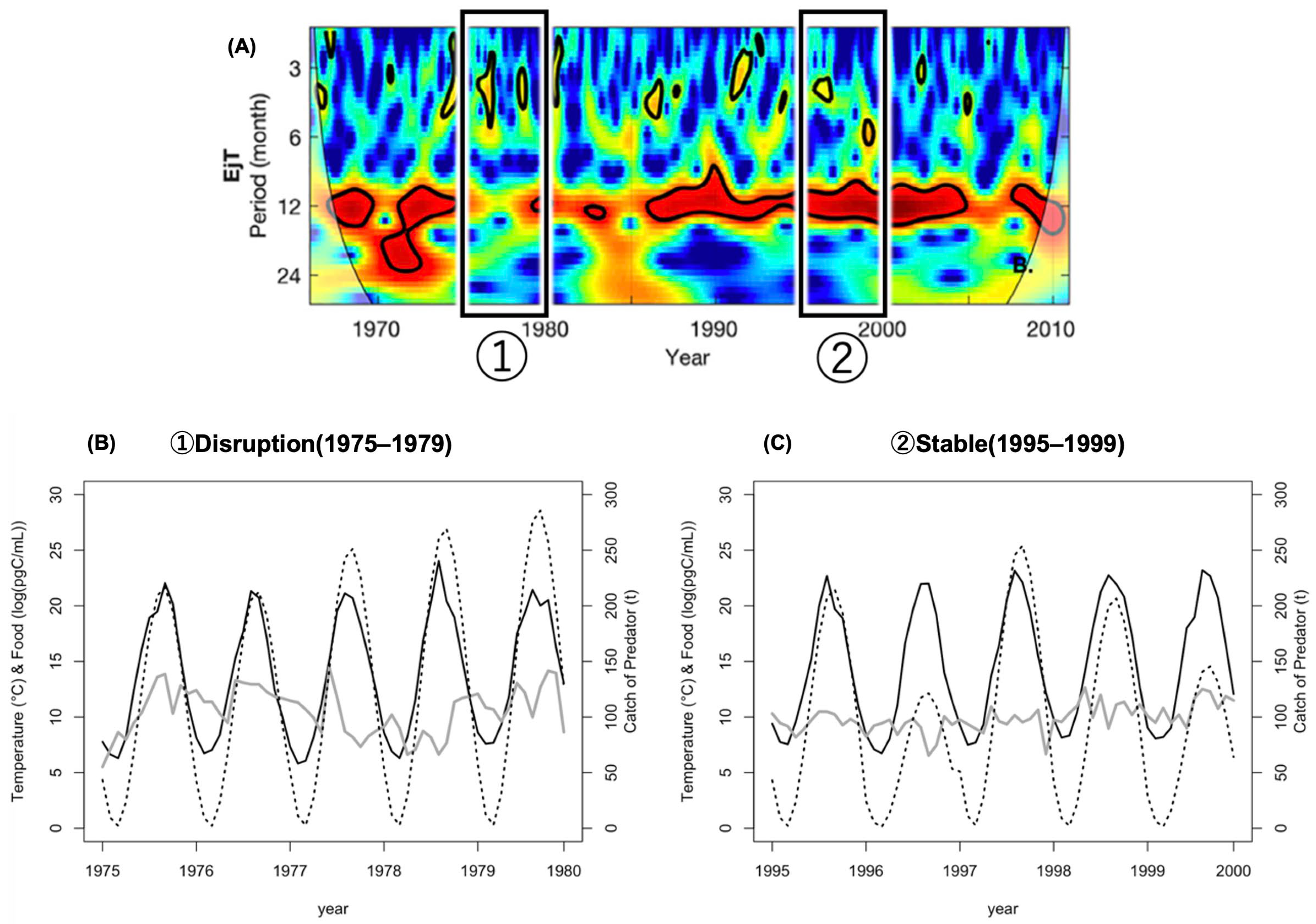
• Disruption period (1975–1979)—when the disruption of the seasonal cycle of this species was observed;
• Stable period (1995–1999)—when its seasonal cycle was stable.

The initial population was set at 1002 individuals (nauplii = 786, copepodite = 12, adults = 204) for the disruption period and 1000 individuals (nauplii = 804, copepodite = 114, adults = 82) for the stable period, based on stage-specific density data for this species in Lake Biwa provided by Dur et al. [27].

After the environment is generated, each individual determines their stage duration under the current water temperature and food concentration, and adults also determine their survival rate under predation pressure. Additionally, females determine their body length (PL) and the number of days required for the first spawning (LT) period under the current conditions.

The initial values of all attributes that agents have are summarized in Table 1.

2.6. Input Data

To identify the main driver of the disruption of the seasonal cycle in the E. japonicus population, we tested the following three scenarios for both periods:

(a)

Set water temperature, food concentration, and predators;

(b)

Set water temperature and food concentration;

(c)

Set water temperature and predators.

The environmental data in Lake Biwa were obtained from the Shiga Prefectural Fisheries Experiment Station (SPFES). The dataset contains monthly surface water temperature (°C), phytoplankton concentration (log pgC/mL), and annual catch of Ayu (Plecoglossus altivelis) and Isaza (Gymnogobius isaza) (t).

The monthly water temperature and food concentration data were linearly interpolated using Re:Mobidyc to convert them into daily data. The annual catch data for Ayu (Plecoglossus altivelis; [19]) and Isaza (Gymnogobius isaza; [54]), the main predators of E. japonicus in Lake Biwa, were used as an indicator of predation pressure. Due to the tendency for higher ayu catch during July and August (https://www.pref.shiga.lg.jp/file/attachment/5238750.pdf (accessed on 14 April 2022)), annual data were transformed into monthly data using a cosine function to align with this seasonal pattern. The monthly catch data were then converted to daily data using the same method as before.

This way, we created two environmental datasets spanning over 5 years (Figure 2B,C). In simulation (b), which excluded the influence of predators, we initially planned not to input any predators. However, without predators, the population of E. japonicus increased infinitely, causing the simulation to crash midway. Therefore, the number of predators was set to a constant value of 50 (t). In simulation (c), the maximum phytoplankton concentrations for each 5-year period (14.5 log pgC/mL and 12.6 log pgC/mL for the disruption and stable period, respectively) were input to exclude the influence of food concentration.

2.7. Submodels

2.7.1. Environmental Conditions

In each timestep, the model extracts water temperature, food concentration and predation pressure from the environmental dataset for the current day. These data are used as variables for the life history traits and reproductive traits defined in the following submodels.

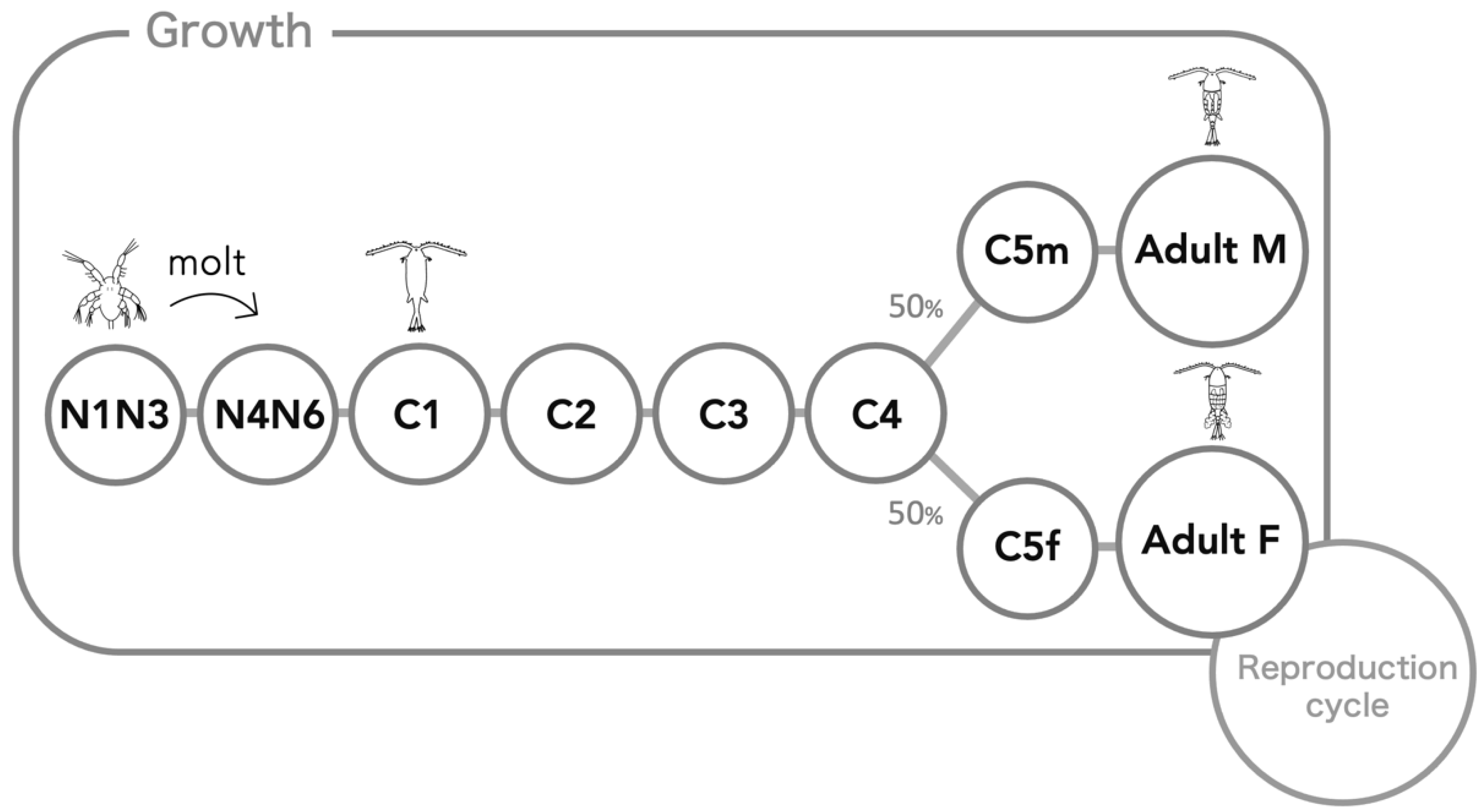
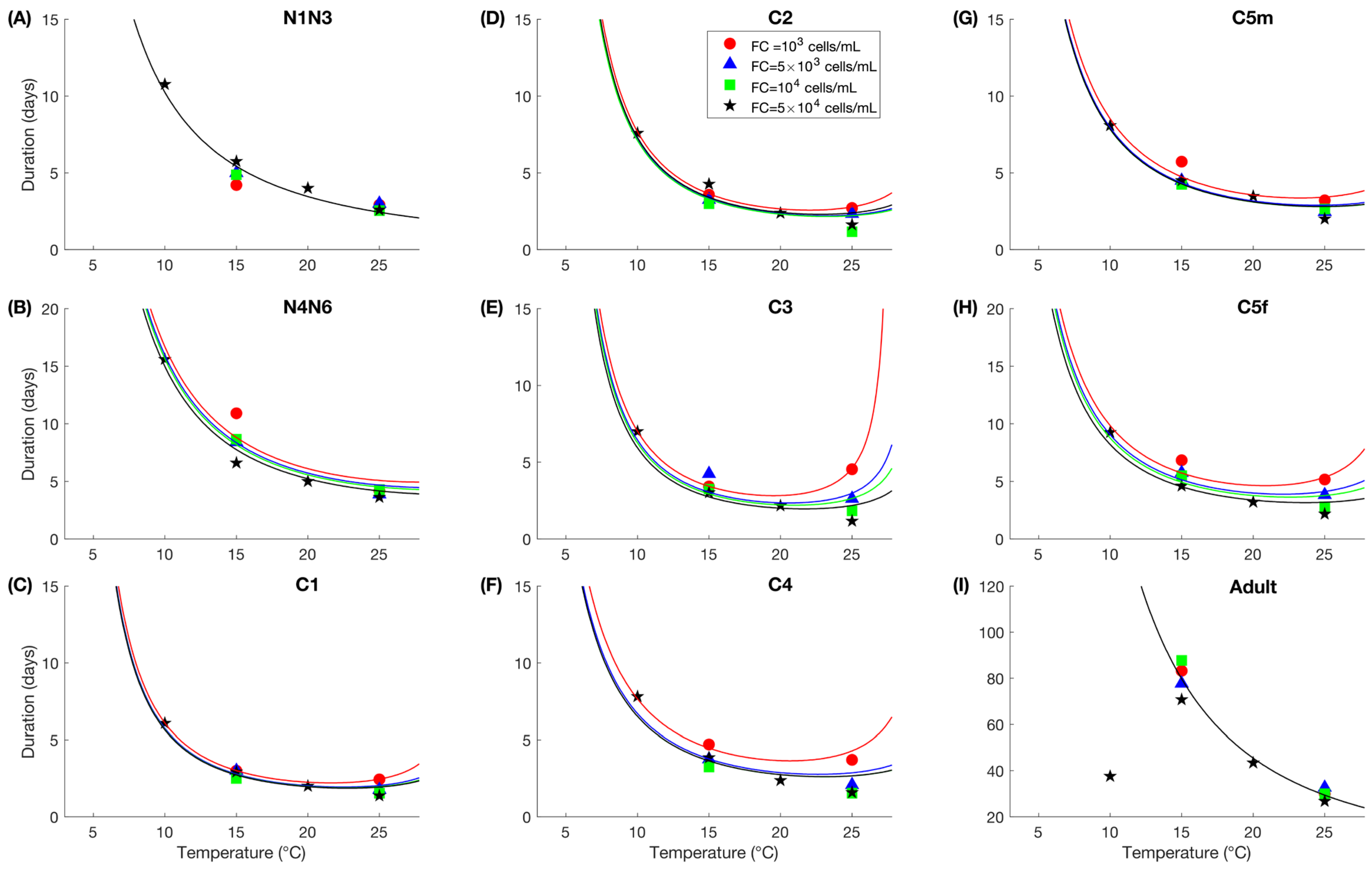
2.7.2. Growth

We used the data from Liu et al. [23,24] to parameterize the growth stages. Liu et al. [23] described the stage duration (D, days) of E. japonicus using the Bĕlehrádek temperature-dependent equation (Equation (1)), which is valid under conditions of sufficient food availability.

$$D=\lambda {(T-a)}^b$$

(1)

where

$\lambda , a$, and $b$ are fitted constants.

$T$ is the water temperature (°C).

However, this species exhibits a characteristic where the negative impact of food shortage becomes more pronounced at higher temperatures [22], which cannot be addressed by the Bĕlehrádek’s equation. Therefore, we applied Kontodimas’ equation (Equation (2)) to better describe and account for this aspect, and fit the equation to the data obtained at each food condition.

$$D=\frac{1}{a{\left(T-T_{min}\right)}^2(T_{max}-T)}$$

(2)

where

$T_{min}$ is the biological minimum temperature (°C).

$T_{max}$ is the biological maximum temperature (°C).

The $T_{max}$ in Kontodimas’ equation was then described using a Gaussian function with food concentration (F, log pgC/mL) as a variable (Equation (3)).

$$T_{max}=a\times exp\left\{-{\left(\frac{F-b}{c}\right)}^2\right\}$$

(3)

where $a, b \mathrm{a}\mathrm{n}\mathrm{d} c$ are fitted constants (Figure S1).

In this way, the adverse effects of low food concentrations at higher temperatures were expressed in a single equation.

Of the 10 growth stages, the adult stage showed no significant difference among food concentrations (KW test, p > 0.01), and the N1N3 stage showed a significant difference but no correlation. Both of these stages were described using the conventional version of Bĕlehrádek’s equation, while the other 8 stages were described using Kontodimas’ equation (Figure 3). We utilized the MATLAB Curve Fitting Toolbox, employing the non-linear least squares method, to achieve the optimal fit for the data. The obtained coefficients in respective equations are summarized in Tables S1 and S2.

Note that in the studies by Liu et al. [23,24], the unit of food concentration was [cells/mL]. We converted it to [log pgC/mL] to align with the unit of field data input into the model. One can refer to Table S1 for details on the conversion method.

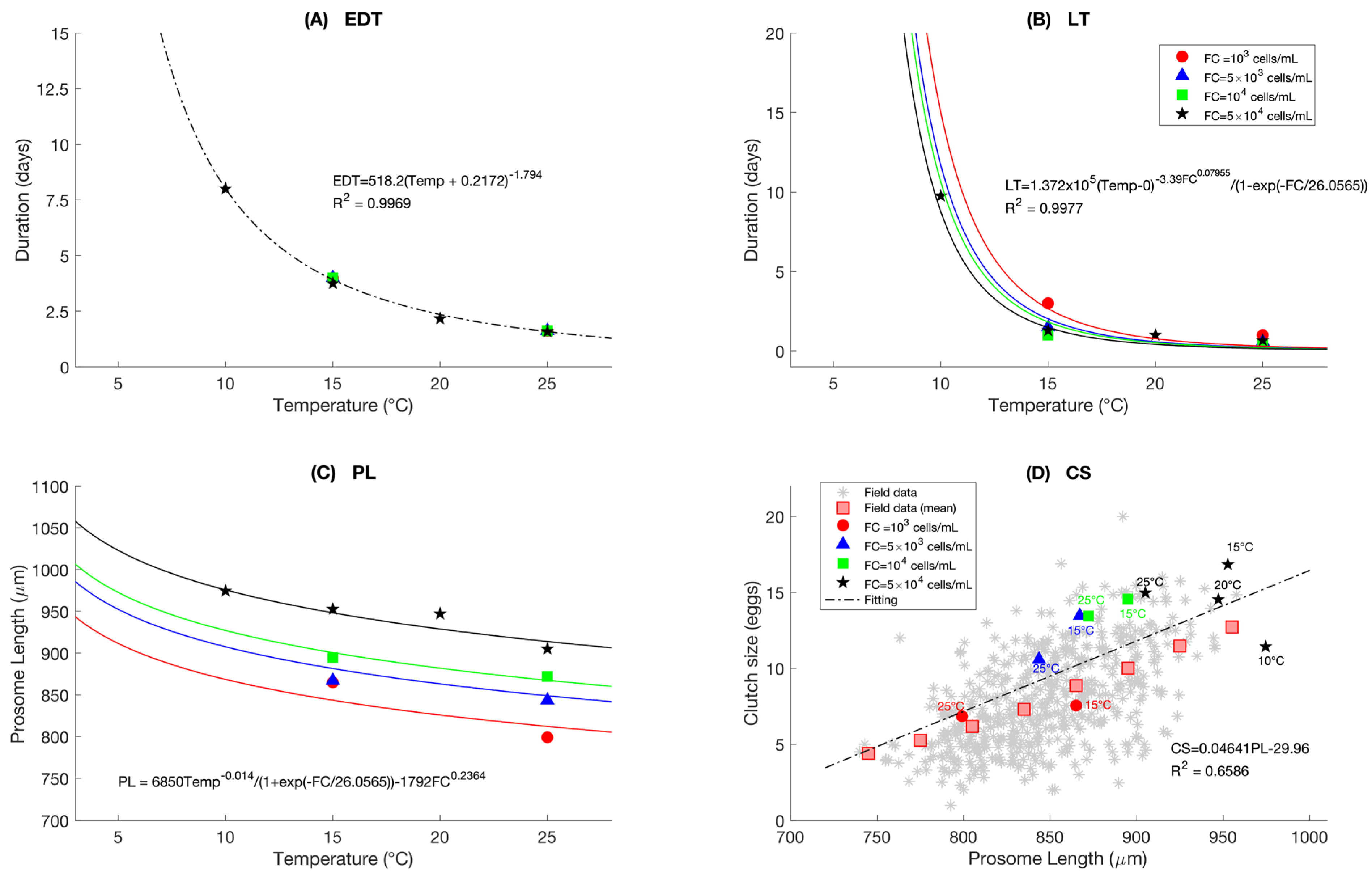
2.7.3. Reproduction

Data from Liu et al. [23,24] and SPFES were used to parameterize the reproductive traits of this species.

Embryonic development time (EDT, days) represents the duration for eggs to hatch. During this period, the nauplii inside the eggs do not consume external food; therefore, EDT is solely influenced by water temperature [22]. Consequently, we described EDT using Bĕlehrádek’s temperature-dependent equation (Equation (1), Figure 4B). On the other hand, latency time (LT, days) is influenced by both water temperature and food availability [22]. Therefore, we expressed LT using the following equation (Equation (4), Figure 4A), which incorporated the food concentration variable into Bělehrádek’s equation, as proposed in Speirs et al. (2005).

$$LT=\lambda {\left(T-a\right)}^b/\left[1-\mathrm{e}\mathrm{x}\mathrm{p}\left(-\frac{F}{F_{max}}\right)\right]$$

(4)

where

$F_{max}$ is the maximum food concentration (26.0565 log pgC/mL).

We utilized the MATLAB Curve Fitting Toolbox, employing the non-linear least squares method, to achieve the optimal fit for the data. The coefficients in the EDL and LT equations are summarized in Table S1.

The effects of water temperature and food concentration on clutch size (CS, eggs/clutch) were implemented indirectly through female body length (PL, µm). We plotted the relationship between CS and female body length and observed that females with larger body lengths tended to produce more eggs. Therefore, CS was described as a linear function dependent on female body length (Equation (5), Figure 4D).

$$\mathrm{CS}=0.04641\mathrm{PL}-29.96$$

(5)

Liu et al. [23] described female body length as a temperature-dependent equation. In this study, we incorporated the data on the relationship between body length and food concentration from Liu et al. [24] into the equation, representing body length as a temperature-food-dependent equation (Equation (6), Figure 4C).

$$\mathrm{PL}=6850T^{-0.014}/\left\{1+exp\left(\frac{-\mathrm{F}}{26.0565}\right)\right\}-1792F^{0.2364}$$

(6)

This equation captures the characteristic of the female body length decreasing with higher water temperatures and lower food concentrations. The values of the parameters in Equation (6) were obtained via the non-linear least squares method of the MATLAB curve fitting toolbox.

Senescence has been observed in egg carrying copepods, with CS decreasing as females grow older [55]. To confirm whether this tendency also exists in this species, we plotted the relationship between female age and CS and observed a gradual decrease in CS as females aged (Figure 5). Therefore, we decided to incorporate the effect of age into CS. The normalized CS data (NormCS) under each temperature–food condition were integrated, and the relationship with age was expressed using Equation (7) (Figure 6).

$$\mathrm{NormCS}=-0.001017{\mathrm{Age}}^{1.36}+1$$

(7)

$$\mathrm{CS}=\mathrm{NormCS} (0.04641\mathrm{PL}-29.96)$$

(8)

Age is the stage duration of E. japonicus adult females (days). By multiplying Equation (7) as a coefficient with Equation (5), the impact of age is considered in CS (Equation (8)).

Hatching success (HS, %) in this species is not influenced by either temperature or food conditions [24]. Therefore, it was fixed at 98.17%, which is the average value obtained in the experimental data [24].

2.7.4. Survival Rate

In Lake Biwa, the main predators of E. japonicus are Ayu and Isaza. A study conducted by Kawabata et al. [11], which examined the stomach contents of Ayu, revealed that 91% of consumed E. japonicus were in the adult stage. Therefore, the impact of predation was exclusively implemented for the adult stage.

When examining the relationship between the total catch of Ayu and Isaza (Predators, t) and the normalized E. japonicus adult individual density (Norm Ad), an observed trend indicated a gradual decrease in density with an increase in predator catch (data obtained from SPFES). As a result, the normalized adult density was expressed as a linear function with the predators catch as a variable (Equation (9), Figure 7).

$$Norm Ad=-2.267\times {10}^{-4}Predators+1$$

(9)

The survival rate of adults (SurvAdult, %/day) was described by multiplying Equation (9) by the mean value of the adult survival rate in Lake Biwa obtained from Kawabata [14] (Equation (10)).

$$SurvAdult=Norm Ad\times 94.3$$

(10)

According to a study examining the stage-specific mortality rates of E. japonicus in Lake Biwa [15], the mortality rate is high for naupliar stages, while it is relatively lower for copepodite stages. In the model, the survival rate for copepodite stages was fixed at 100% and for nauplii (SurvN, %/day), it was derived from seasonal data in Kawabata [14] and expressed by the following equation.

$$SurvN=94-\frac{12}{2}cos\left(\frac{2\pi }{365}(Time-180)\right)$$

(11)

In the above equation, $Time$ is the cumulative simulation time step. The values of the parameters in Equation (11) were obtained via the non-linear least squares method of the MATLAB curve fitting toolbox.

2.7.5. Individual Variability

We implemented individual variabilities in all stage durations, reproductive traits (EDT, LT, PL, CS, and Age), and adult density. For this purpose, we first separated the contribution of extrinsic factors from the intrinsic individual variability. For that, the data from different experimental conditions were combined and normalized from the condition effects.

$$z_{ij}=x_{ij}/{\overline{x}}_j$$

(12)

x_ij is the observed value of the parameter for individual i during the experiment j, z_ij is the corresponding value of the data normalized and ${\overline{x}}_j$ is the mean value of the parameter during the experiment j.

Stage durations, EDT, and LT were represented by a gamma distribution according to Liu et al. [24]. To estimate the shape parameter (α) and scale parameter (β) values, we fitted the normalized duration data with the ‘gamcdf’ function [x/α, β] in MATLAB (MathWorks Inc. 2017) using the lowest non-linear least squares method (Figure 8 and Figure 9). Meanwhile, the variability in PL, CS, age, and adult density was expressed using normal distributions (Figure 9), determined based on the results of the Kolmogorov–Smirnov test (p < 0.05).

2.8. Model Verification

The proper implementation of the model was assessed through a comparison of its outputs with the experimental results of Liu et al. [24]. Simulations were conducted under identical water temperature and food concentrations as in the referenced study, enabling a throughout evaluation of stage durations and reproductive parameters against the empirical data. Due to the limited number of observations for some conditions, the statistical power of the analysis would be compromised, making robust statistical analysis challenging. Instead, we confirmed the proper functioning of the model by ensuring that the variability range of the experimental data aligned with our model output. The model exhibits commendable agreement with the experimental results at all food concentrations when the temperature was 15 °C (Figure 10). However, at 25 °C, discrepancies emerged in some stage durations between the model outputs and experimental results, particularly under higher food conditions. These discrepancies arise from the utilization of the lowest food concentration as the baseline during the parameterizing of food effects (Figure 3). Given that the maximum phytoplankton concentration in Lake Biwa may or may not reach the minimum food concentration during the experiment, it was concluded that these observed discrepancies under higher food conditions do not significantly impact the main simulations.

3. Results

3.1. Simulation (a)—Effects of Water Temperature, Food Concentration, and Predators

The simulation incorporating water temperature, food concentration, and predator data during the period of disruption (1975–1979) revealed a lack of regular seasonal fluctuations in the E. japonicus population, manifesting a steady decline in density over the years (Figure 11A). Conversely, the simulation for the stable period (1995–1999) exhibits regular seasonal peaks in population fluctuations, indicating a more stable dynamic (Figure 11B). Wavelet analysis of these outputs reveals that the seasonal cycle of the population was interrupted in the middle of 1977 in the simulation for the disruption period (Figure 11C). In contrast, the simulation for the stability period demonstrated a consistent and stable seasonal cycle throughout the five years (Figure 11D).

3.2. Simulation (b)—Effects of Water Temperature and Food Concentration

Excluding the influence of predators in the simulations for both the disruption period and stable period resulted in the emergence of regular seasonal peaks in population fluctuations, with nearly identical waveforms for both periods (Figure 12A,B). Wavelet analysis, employed to scrutinize the periodicity of population fluctuations in each simulation, unveiled a robust and sustained seasonal cycle persisting over the course of five-year duration for both periods (Figure 12C,D).

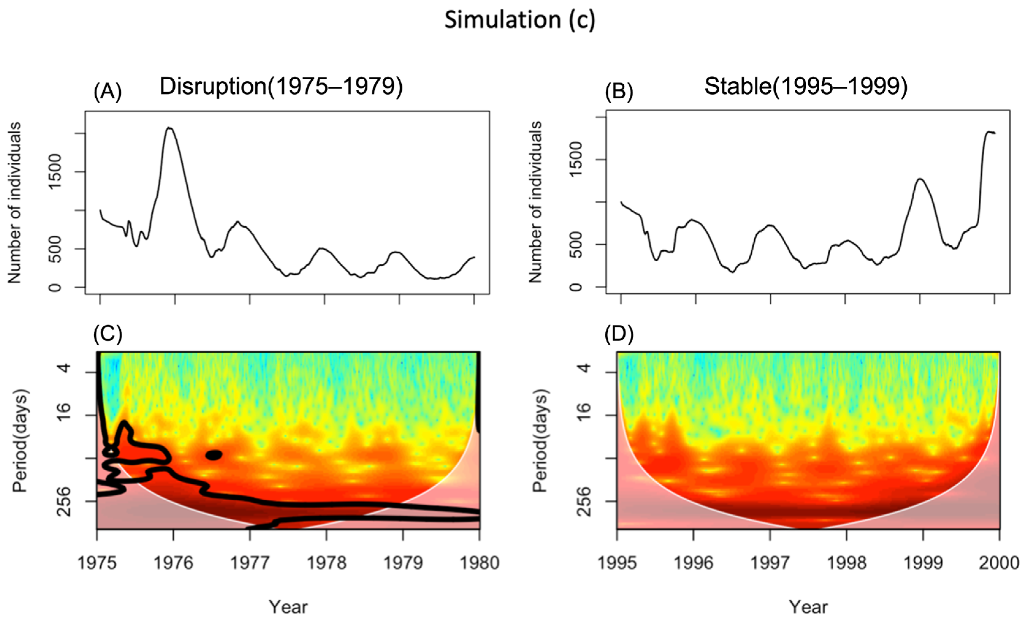
3.3. Simulation (c)—Effects of Water Temperature and Predation

In the simulation that excluded the influence of food, regular peaks were observed in the population fluctuations of both the disruption and stable periods (Figure 13A,B). Wavelet analysis revealed a strong seasonal cycle throughout the five-year period in the simulation of the disruption period (Figure 13C,D). Although no significant differences were observed in the stable period, a distinct red line was noted in the one-year cycle.

4. Discussion

In this study, we investigated the hypothesis that the disruption in the seasonal cycle of E. japonicus’ population density observed over the past 45 years is due to the effects of water temperature, predators’ pressure, and food conditions, using simulations with IBM. To identify the main environmental parameter causing their disruption, three scenarios were conducted by varying combinations of input environmental data.

4.1. The Simulation Results

Disruptions in population fluctuations in the simulation (1975–1979) were observed only when inputting three environmental factors, water temperature, food, and predators. Removing the effects of either predators or food resulted in stable seasonal cycles throughout the 5-year period, suggesting that the disruption in the seasonal cycle of E. japonicus in Lake Biwa was likely caused by both food conditions and predators. The results from simulations (b) and (c) also suggest that the impact on population size is more pronounced from predators rather than food conditions. This finding is consistent with the analysis of Liu et al. [10] who investigated zooplankton samples from Lake Biwa. In their results, the long-term trend of zooplankton biomass in the lake was mostly influenced by fish predation rather than nutritional conditions and global warming. According to Gerten and Adrian [56] who examined the impact of warming on the annual peak abundance of three copepod species in Müggelsee (Germany), temperate species do not respond noticeably to the warming trend. On the other hand, Winder et al. [57] investigated the population dynamics of the cold-adapted calanoid copepod Leptodiaptomus ashlandi in Lake Washington (USA) and suggested that the seasonal cycle of this species was revealed to be influenced by the warming of water temperature and fluctuations in phytoplankton availability. Our results and these previous studies indicate that food conditions and predators, rather than water temperature, could drive seasonal fluctuations in temperate copepod species.

4.2. Comparison of Simulation Output and Field Population Density

When comparing the simulated population numbers with the observed individual density in the field, the timing of the peaks did not match (Figure S2). Since the positions of the peaks remained consistent even when altering the combinations of input environmental factors, water temperature could be the dominant factor. In the field data, the peak of water temperature and the peak of the population density of this species generally occur around the same time (Figure S3). However, in the simulation, the peak in population numbers occurs after the peak in water temperature. This is likely because the current model does not consider temperature-dependent survival rates. According to the experiments conducted by Liu et al. [23], which investigated the relationship between water temperature and life history traits of this species, there was a tendency for survival rates to decrease when the water temperature was lowered from 25 °C to 10 °C under conditions of abundant food. As the current model has not incorporated this aspect, the decrease in population numbers is represented as a reduction in productivity due to the prolonged duration of growth stages, EDT and LT under low temperatures. For this reason, there is a time lag before the effects of changes in water temperature become apparent. In the future, it would be desirable to implement temperature-dependent survival rates.

The discrepancy in peaks could also be attributed to the possibility that the data used as an indicator of food condition were not appropriate. In this study, the data of phytoplankton concentration in Lake Biwa (excluding cyanobacteria and sizes larger than 100 µm, which cannot be consumed by this species) were input into the model. However, E. japonicus is an omnivorous copepod that could also consume bacteria [58], microzooplankton and detritus [59,60]. Hence, the influence of food concentration could be underestimated in the current simulation. Liu et al. [25] developed a size-dependent food index (f) as an indicator of food for omnivorous copepods. This index (f) can be incorporated into the IBM by implementing the Dynamic Energy Budget (DEB) theory, which focuses on the energy flow from food intake.

4.3. The Predators’ Effect in the Model

In this study, we adopted simple mortality rates, which are most commonly used in NPZ models (nutrient–phytoplankton–zooplankton models) and are typically described as $\mu =\gamma \left(d,Z\right)$, dependent on a constant mortality rate (d) and the biomass of zooplankton (Z) [61]. Here, we replaced Z with a function of predator catch and adult population density to describe the predation pressure, but this approach is quite simplistic. In the European Regional Sea Ecosystem Model (ERSEM) proposed by Bryant et al. [62], zooplankton mortality rates due to predation are estimated using consumption rates and biomasses of potential predators. This approach requires a lot of data and knowledge of predator consumption rates, leading to mortality rates strongly influenced by available observations. Therefore, it is not advisable to apply it in long-term simulations where ecosystem dynamics and zooplankton characteristics may have changed [61]. In size-structured models such as those proposed by Maury et al. [63] and Baird and Suthers [64], zooplankton mortality including predation is implicitly parameterized when size classes larger than zooplankton are incorporated. However, the mechanistic formulation of the predation term needs several parameters such as assimilation efficiency, preferred size range and swimming speed of the predator. To avoid the parameterization problems, Zhou et al. [65] introduced the size spectrum zooplankton closure model, which is driven by phytoplankton biomass, temperature, and the mean slope of the biomass spectrum. While the model tended to overestimate, it has a high potential to adequately simulate seasonal changes in zooplankton dynamics. Regardless of the approach taken, improving the accuracy of predation mortality rates requires additional data on predators.

Due to the availability of only annual data for predator catch, we used monthly data adjusted to align with the typical peak period of Ayu, which usually occurs after June or July each year. However, the observed increase in Ayu catch around these periods may be related to concentrated fishing activities during this time (https://www.pref.shiga.lg.jp/file/attachment/5439316.pdf (accessed on 14 April 2022)). Additionally, Ayu in Lake Biwa are subject to a fishing ban from 21 August to 20 November. During this period, from early September to late October, it is the spawning season. It remains uncertain during which specific seasons Ayu are more abundant. According to the SPFES report that estimated the current stock of Ayu in Lake Biwa using a growth-survival model (https://www.pref.shiga.lg.jp/file/attachment/2022840.pdf (accessed on 14 April 2022)), there is a positive correlation between the estimated stock and the catch for each year, but it is not very strong (r = 0.613). In particular, there is significant divergence in years with high stock levels, indicating that catch is influenced by demand. Although some previous studies have used catch data as an indicator of predation pressure [10,27], this indicator may not be appropriate. As mentioned above, detailed data on predators will be necessary in future development, or alternatively, using predator abundance estimated by the growth-survival model might be considered.

4.4. Future Development and Model Potential

Cyclopoida spp. inhabiting Lake Biwa are known to prey on the nauplii of E. japonicus [16]. Although this study represents the survival rate of the nauplii stage as seasonal, future modeling efforts should aim to incorporate the effects of predation by Cyclopoida spp. Additionally, research by Gao et al. [26] demonstrated that among the three major zooplankton species in Lake Biwa, E. japonicus is the most vulnerable to acidic stress, indicating that acute acidic stress from acid rain may impact zooplankton community structures. Therefore, future model improvements could include incorporating the effects of pH on survival rates and metabolism.

Future studies utilizing our individual-based model (IBM) should prioritize rigorous model validation and scenario testing by simulating realistic ecological scenarios and comparing model outputs with empirical data. This approach will facilitate a deeper understanding of system dynamics and enhance predictive capabilities regarding responses to environmental changes or management interventions. Lake Biwa monitoring programs present opportunities for further model refinement by comparing model outputs with in situ data collected through year-long monitoring experiments. Integrating fish predator abundance data into monitoring efforts will further enhance model validation and provide insights into real-world applicability.

In comparison to multivariate analyses, our IBM offers several advantages. While Canonical Correspondence Analysis (CCA) or Principal Component Analysis (PCA) are useful for exploring relationships between variables and communities, IBMs provide a unique framework for studying ecological dynamics by incorporating individual-based processes, biological realism, nonlinear relationships, and spatial–temporal complexity. The choice of modeling approach ultimately depends on specific research questions, system complexity, and desired levels of detail in understanding population dynamics and ecosystem responses.

Furthermore, the structure of our model can be adapted to other diaptomid copepods that exhibit comparable reproductive and life cycle characteristics to E. japonicus. This adaptation primarily involves parameter calibration and the inclusion of relevant environmental data specific to the target species.

Our model’s findings underscore the key role of fish in the trophic dynamics of lakes [66] and highlight the importance of considering multiple trophic levels to develop effective predictive and management tools. With an improved version of our model, we can forecast the stage composition of dominant calanoid copepods and assess the health of the zooplankton community. Given the role of copepods as indicators of the health status of continental aquatic ecosystems [67], this information is crucial for the conservation and preservation of Lake Biwa.

5. Conclusions

In conclusion, this study demonstrated the impacts of food concentration and predators on the seasonal cycle of population fluctuations in the copepod E. japonicus in Lake Biwa. This advancement is important for investigating the impacts of environmental changes on Lake Biwa’s food web, given that this species has dominated the zooplankton community in the lake for over 50 years. As demonstrated in this study, the seasonal cycle of this species is influenced by both food availability and predators. The presence of predators strongly changes the model predictions. Since this model is relatively simple, it would be desirable to implement factors such as temperature-dependent survival rates, relevant data on food sources and predators, and interaction between individuals to enhance the accuracy of the model. The application of such refined models will advance the understanding of the relationship between environmental factors and copepods.

References

- Adrian, R.; Wilhelm, S.; Gerten, D. Life-history traits of lake plankton species may govern their phenological response to climate warming. Glob. Change Biol. 2006, 12, 652–661. [Google Scholar] [CrossRef]
- Nakazawa, T.; Doi, H. A perspective on match/mismatch of phenology in community contexts. Oikos 2012, 121, 489–495. [Google Scholar] [CrossRef]
- Kawanabe, H.; Nishino, M.; Maehata, M. Lake Biwa: Interactions between Nature and People, 1st ed.; Springer: Berlin/Heidelberg, Germany, 2012. [Google Scholar] [CrossRef]
- Tsugeki, N.; Oda, H.; Urabe, J. Fluctuation of the zooplankton community in Lake Biwa during the 20th century: A paleolimnological analysis. Limnology 2003, 4, 101–107. [Google Scholar] [CrossRef]
- Hyodo, F.; Tsugeki, N.; Azuma, J.; Urabe, J.; Nakanishi, M.; Wada, E. Changes in stable isotopes, lignin-derived phenols, and fossil pigments in sediments of Lake Biwa, Japan: Implications for anthropogenic effects over the last 100 years. Sci. Total Environ. 2008, 403, 139–147. [Google Scholar] [CrossRef]
- Hsieh, C.H.; Sakai, Y.; Ban, S.; Ishikawa, K.; Ishikawa, T.; Ichise, S.; Yamamura, N.; Kumagai, M. Eutrophication and warming effects on long-term variation of zoo- plankton in Lake Biwa. Biogeosciences 2011, 8, 1383–1399. [Google Scholar] [CrossRef]
- Okubo, T.; Azuma, Y. Last 35 years variation for water quality and watershed environments in Lake Biwa. Trans. Res. Inst. Oceanochem. 2016, 29, 2–16. (In Japanese) [Google Scholar]
- Hsieh, C.H.; Ishikawa, K.; Sakai, Y.; Ishikawa, T.; Ichise, S.; Yamamoto, Y.; Kuo, T.C.; Park, H.D.; Yamamura, N.; Kumagai, M. Phytoplankton community reorganization driven by eutrophication and warming in Lake Biwa. Aquat. Sci. 2010, 72, 467–483. [Google Scholar] [CrossRef]
- Maehata, M. Environmental conservation of Lake Biwa. In Lake Biwa: Interactions between Nature and People; Kawanabe, H., Nishino, M., Maehata, M., Eds.; Springer: Dordrecht, The Netherlands, 2012; pp. 419–513. [Google Scholar] [CrossRef]
- Liu, X.; Dur, G.; Ban, S.; Sakai, Y.; Ohmae, S.; Morita, T. Planktivorous fish predation masks anthropogenic disturbances on decadal trends in zooplankton biomass and body size structure in Lake Biwa, Japan. Limnol. Oceanogr. 2020, 65, 667–682. [Google Scholar] [CrossRef]
- Kawabata, K.; Narita, T.; Nagoshi, M.; Nishino, M.; Kawabata, K.; Nagoshi, M.; Nishino, M. Stomach contents of the landlocked dwarf ayu in Lake Biwa, Japan. Limnology 2002, 3, 135–142. [Google Scholar] [CrossRef]
- Kawabata, K. Abundance and distribution of Eodiaptomus japonicus (Copepoda: Calanoida) in Lake Biwa. Bull. Plankton Soc. Jpn. 1987, 34, 173–183. [Google Scholar]
- Kawabata, K. Seasonal changes in abundance and vertical distribution of Mesocyclops thermocyclopoides, Cyclops vicinus and Daphnia longispina in Lake Biwa. Jpn. J. Limnol. 1989, 50, 9–13. [Google Scholar] [CrossRef]
- Kawabata, K. Mortality Rate of Eodiaptomus japonicus (Copepoda: Calanoida) in Lake Biwa. Jpn. J. Limnology 1993, 54, 131–136. [Google Scholar] [CrossRef]
- Kawabata, K. Ontogenetic niches of a planktonic copepod in Lake Biwa studied on a fine temporal scale. Ecol. Res. 1995, 10, 207–215. [Google Scholar] [CrossRef]
- Kawabata, K. Clearance rate of the cyclopoid copepod Mesocyclops dissimilis on the calanoid copepod Eodiaptomus japonicus. Plankton Benthos Res. 2006, 1, 68–70. [Google Scholar] [CrossRef]
- Kawabata, K.; Urabe, J. Population dynamics of planktonic crustacea studied during BITEX’93. Jpn. J. Limnol. 1996, 57, 545–552. [Google Scholar] [CrossRef]
- Kawabata, K.; Narita, T. Feeding rate of naupliar Eodiaptomus japonicus. Plankton Biol. Ecol. 2003, 50, 27–29. [Google Scholar]
- Kawabata, K.; Narita, T.; Nishino, M. Predator–prey relationship between the landlocked dwarf ayu and planktonic crustacea in Lake Biwa, Japan. Limnology 2006, 7, 199–203. [Google Scholar] [CrossRef]
- Nagata, T.; Okamoto, K. Filtering rates on natural bacteria by Daphnia longispina and Eodiaptomus japonicus in Lake Biwa. J. Plankton Res. 1988, 10, 835–850. [Google Scholar] [CrossRef]
- Liu, X.; Ban, S. Effects of acclimatization on metabolic plasticity of Eodiaptomus japonicus (Copepoda: Calanoida) determined using an optical oxygen meter. J. Plankton Res. 2017, 39, 111–121. [Google Scholar] [CrossRef]
- Liu, X.; Ban, S. Effects of temperature and nutritional conditions on physiological responses of the freshwater copepod Eodiaptomus japonicus in Lake Biwa, (Japan). Limnol. Study 2018, 5, 13–24. [Google Scholar]
- Liu, X.; Beyrend-Dur, D.; Dur, G.; Ban, S. Effects of temperature on life history traits of Eodiaptomus japonicus (Copepoda: Calanoida) from Lake Biwa (Japan). Limnology 2014, 15, 85–97. [Google Scholar] [CrossRef]
- Liu, X.; Beyrend, D.; Dur, G.; Ban, S. Combined effects of temperature and food concentration on growth and reproduction of Eodiaptomus japonicus (Copepoda: Calanoida) from Lake Biwa (Japan). Freshw. Biol. 2015, 60, 2003–2018. [Google Scholar] [CrossRef]
- Liu, X.; Dur, G.; Ban, S.; Sakai, Y.; Ohmae, S.; Morita, T. Quasi-decadal periodicities in growth and production of the copepod Eodiaptomus japonicus in Lake Biwa, Japan, related to the Arctic Oscillation. Limnol. Oceanogr. 2021, 66, 3783–3795. [Google Scholar] [CrossRef]
- Gao, H.; Liu, X.; Ban, S. Effect of acute acidic stress on survival and metabolic activity of zooplankton from Lake Biwa, Japan. Inland Waters 2022, 12, 488–498. [Google Scholar] [CrossRef]
- Dur, G.; Liu, X.; Sakai, Y.; Hsieh, C.H.; Ban, S.; Souissi, S. Disrupted seasonal cycle of the warm-adapted and main zooplankter of Lake Biwa, Japan. J. Great Lakes Res. 2022, 48, 1206–1218. [Google Scholar] [CrossRef]
- Halsband-Lenk, C.; Carlotti, F.; Greve, W. Life-history strategies of calanoid congeners under two different climate regimes: A comparison. ICES J. Mar. Sci. 2004, 61, 709–720. [Google Scholar] [CrossRef]
- Herzig, A. The ecological significance of the relationship between temperature and duration of embryonic development in planktonic freshwater copepods. Hydrobiologia 1983, 100, 65–91. [Google Scholar] [CrossRef]
- Ban, S. Effect of temperature and food concentration on post-embryonic development, egg production and adult body size of calanoid copepod Eurytemora affinis. J. Plankton Res. 1994, 16, 721–735. [Google Scholar] [CrossRef]
- Jiménez-Melero, R.; Santer, B.; Guerrero, F. Embryonic and naupliar development of Eudiaptomus gracilis and Eudiaptomus graciloides at different temperatures: Comments on individual variability. J. Plankton Res. 2005, 27, 1175–1187. [Google Scholar] [CrossRef]
- Kiørboe, T.; Møhlenberg, F.; Hamburger, K. Bioenergetics of the planktonic copepod Acartia tonsa: Relation between feeding, egg production and respiration, and composition of specific dynamic action. Mar. Ecol. Prog. Ser. 1985, 26, 85–97. [Google Scholar] [CrossRef]
- Klein Breteler, W.C.M.; Gonzalez, S.R.; Schogt, N. Development of Pseudocalanus elongatus (Copepoda, Calanoida) cultured at different temperature and food conditions. Mar. Ecol. Prog. Ser. 1995, 119, 99–110. [Google Scholar] [CrossRef]
- Jiménez-Melero, R.; Parra, G.; Guerrero, F. Effect of temperature, food and individual variability on the embryonic development time and fecundity of Arctodiaptomus salinus (Copepoda: Calanoida) from a shallow saline pond. Hydrobiologia 2012, 686, 241–256. [Google Scholar] [CrossRef]
- Lee, H.; Ban, S.; Ikeda, T.; Matsuishi, T. Effect of temperature on development growth and reproduction in the marine copepod Pseudocalanus newmani at satiating food condition. J. Plankton Res. 2003, 25, 261–271. [Google Scholar] [CrossRef]
- Svensson, J.E. Fish predation on Eudiaptomus gracilis in relation to clutch size, body size, and sex: A field experiment. Hydrobiologia 1997, 344, 155–161. [Google Scholar] [CrossRef]
- Jeppesen, E.; Jensen, J.P.; Søndergaard, M.; Lauridsen, T.; Pedersen, L.J.; Jensen, L. Top-down control in fresh-water lakes: The role of nutrient state, submerged macrophytes and water depth. Hydrobiologia 1997, 342, 151–164. [Google Scholar] [CrossRef] [PubMed]
- Verheye, H.M.; Richardson, A.J.; Hutchings, L.; Marska, G.; Gianakouras, D. Long-term trends in the abundance and community structure of coastal zooplankton in the southern Benguela system, 1951–1996. Afr. J. Mar. Sci. 1998, 19, 317–332. [Google Scholar] [CrossRef]
- Daskalov, G.M. Overfishing drives a trophic cascade in the Black Sea. Mar. Ecol. Prog. Ser. 2002, 225, 53–63. [Google Scholar] [CrossRef]
- Brooks, J.L.; Dodson, S.I. Predation, body size, and composition of plankton. Science 1965, 150, 28–35. [Google Scholar] [CrossRef]
- Rettig, J.E. Zooplankton responses to predation by larval bluegill: An enclosure experiment. Freshw. Biol. 2003, 48, 636–648. [Google Scholar] [CrossRef]
- Hambright, K.D. Long-term zooplankton body size and species changes in a subtropical lake: Implications for lake management. Fundam. Appl. Limnol. Arch. Hydrobiol. 2008, 173, 1–13. [Google Scholar] [CrossRef]
- Dorman, J.G.; Sydeman, W.J.; Bograd, S.J.; Powell, T.M. An individual-based model of the krill Euphausia pacifica in the California current. Prog. Oceanogr. 2015, 138, 504–520. [Google Scholar] [CrossRef]
- Xu, Y.; Rose, K.A.; Chai, F.; Chavez, F.P.; Ayon, P. Does spatial variation in environmental conditions affect recruitment? A study using a 3-D model of Peruvian anchovy. Prog. Oceanogr. 2015, 138, 417–430. [Google Scholar] [CrossRef]
- Stillman, R.A.; Railsback, S.F.; Giske, J.; Berger, U.; Grimm, V. Making predictions in a changing world: The benefits of individual-based ecology. BioScience 2015, 65, 140–150. [Google Scholar] [CrossRef]
- DeAngelis, D.L.; Mooij, W.M. Individual-based modeling of ecological and evolutionary processes. Annu. Rev. Ecol. Evol. Syst. 2005, 36, 147–168. [Google Scholar] [CrossRef]
- Grimm, V.; Railsback, S. Individual-Based Modeling and Ecology; Princeton University Press: Princeton, NJ, USA, 2005. [Google Scholar] [CrossRef]
- Grimm, V.; Berger, U.; Bastiansen, F.; Eliassen, S.; Ginot, V.; Giske, J.; Goss-Custard, J.; Grand, T.; Heinz, S.K.; Huse, G.; et al. A standard protocol for describing individual-based and agent-based models. Ecol. Model. 2006, 198, 115–126. [Google Scholar] [CrossRef]
- Grimm, V.; Berger, U.; DeAngelis, D.L.; Polhill, J.G.; Giske, J.; Railsback, S.F. The ODD protocol: A review and first update. Ecol. Model. 2010, 221, 2760–2768. [Google Scholar] [CrossRef]
- Grimm, V.; Railsback, S.F.; Vincenot, C.E.; Berger, U.; Gallagher, C.; Deangelis, D.L.; Edmonds, B.; Ge, J.; Giske, J.; Groeneveld, J.; et al. The ODD protocol for describing agent-based and other simulation models: A second update to improve clarity, replication, and structural realism. JASSS 2020, 23, 7. [Google Scholar] [CrossRef]
- El Messoussi, S.; Hafid, H.; Lahrouni, A.; Afif, M. Simulation of Temperature Effect on the Population Dynamic of the Mediterranean Fruit Fly Ceratitis capitata (Diptera; Tephritidae). J. Agron. 2007, 6, 374–377. [Google Scholar] [CrossRef]
- Souissi, S.; Ban, S. The consequence of individual variability in moulting probability and the aggregation of stages for modelling copepod population dynamics models. J. Plankton Res. 2001, 23, 1279–1296. [Google Scholar] [CrossRef]
- Dur, G.; Souissi, S.; Devreker, D.; Ginot, V.; Schmitt, F.G.; Hwang, J.S. An individual-based model to study the reproduction of egg bearing copepods: Application to Eurytemora affinis (Copepoda Calanoida) from the Seine estuary, France. Ecol. Model. 2009, 220, 1073–1089. [Google Scholar] [CrossRef]
- Briones, J.C.; Tsai, C.-H.; Nakazawa, T.; Sakai, Y.; Papa, R.D.S.; Hsieh, C.; Okuda, N. Long-term changes in the diet of Gymnogobius isaza from Lake Biwa, Japan: Effects of body size and environmental prey availability. PLoS ONE 2012, 7, e53167. [Google Scholar] [CrossRef] [PubMed]
- Devreker, D.; Pierson, J.J.; Souissi, S.; Kimmel, D.G.; Roman, M.R. An experimental approach to estimate egg production and development rate of the calanoid copepod Eurytemora affinis in Chesapeake Bay, USA. J. Exp. Mar. Biol. Ecol. 2012, 416–417, 72–83. [Google Scholar] [CrossRef]
- Gerten, D.; Adrian, R. Species-specific changes in the phenology and peak abundance of freshwater copepods in response to warm summers. Freshw. Biol. 2002, 47, 2163–2173. [Google Scholar] [CrossRef]
- Winder, M.; Schindler, D.E.; Essington, T.E.; Litt, A.H. Disrupted seasonal clockwork in the population dynamics of a freshwater copepod by climate warming. Limnol. Oceanogr. 2009, 54 6Pt 2, 2493–2505. [Google Scholar] [CrossRef]
- Burnsd, C.W.; Hegarty, B. Diet selection by copepods in the presence of cyanobacteria. J. Plankton Res. 1994, 16, 1671–1690. [Google Scholar] [CrossRef]
- Poulet, S.A. Factors controlling utilization of non-a1ga1 diets by particle-grazing copepods. Oceanol. Acta 1983, 6, 221–234. [Google Scholar]
- Kiørboe, T. Fluid dynamic constraints on resource acquisition in small pelagic organisms. Eur. Phys. J. Spec. Top. 2016, 225, 669–683. [Google Scholar] [CrossRef]
- Daewel, U.; Hjøllo, S.S.; Huret, M.; Ji, R.; Maar, M.; Niiranen, S.; Travers-Trolet, M.; Peck, M.A.; van de Wolfshaar, K.E. Predation control of zooplankton dynamics: A review of observations and models. ICES J. Mar. Sci. 2014, 71, 254–271. [Google Scholar] [CrossRef]
- Bryant, A.D.; Heath, M.R.; Broekhuizen, N.; Ollason, J.G.; Gurney, W.S.C.; Greenstreet, S.P.R. Modeling the predation, growth and population dynamics of fish within a spatially-resolved shelf-sea ecosystem model. Neth. J. Sea Res. 1995, 33, 407–421. [Google Scholar] [CrossRef]
- Maury, O.; Faugeras, B.; Shin, Y.-J.; Poggiale, J.-C.; Ari, T.B.; Marsac, F. Modeling environmental effects on the size-structured energy flow through marine ecosystems. Part 1: The model. Prog. Oceanogr. 2007, 74, 479–499. [Google Scholar] [CrossRef]
- Baird, M.E.; Suthers, I.M. A size-resolved pelagic ecosystem model. Ecol. Model. 2007, 203, 185–203. [Google Scholar] [CrossRef]
- Zhou, M.; Carlotti, F.; Zhu, Y. A size-spectrum zooplankton closure model for ecosystem modelling. J. Plankton Res. 2010, 32, 1147–1165. [Google Scholar] [CrossRef]
- Jeppesen, E.; Meerhoff, M.; Holmgren, K.; González-Bergonzoni, I.; Teixeira de Mello, F.; Declerck, S.; De Meester, L.; Søndergaard, M.; Lauridsen, T.L.; Bjerring, R.; et al. Impacts of climate warming on lake fish community structure and potential effects on ecosystem function. Hydrobiologia 2010, 646, 73–90. [Google Scholar] [CrossRef]
- Jaime, S.; Cervantes-Martínez, A.; Gutiérrez-Aguirre, M.A.; Jùares-Morales, J.R.; Reyes-Solares, E.M.; Delgado-Blas, V.H. Historical zooplankton composition indicates eutrophication stages in a Neotropical aquatic system: The case of Lake Amatitlàn, Central America. Diversity 2021, 13, 432. [Google Scholar] [CrossRef]