Abstract
Because of their wide distribution, short life cycle, rapid reproduction, and sensitivity to the environment, rodents can indicate changes in habitat quality and climate variables. Long-term studies are needed to verify these changes and assumptions about their causes. We analyzed small mammal trapping data in Lithuania, covering the period 1975–2023, with 1821 trapping sites and 57,426 small mammal individuals, with a focus on the bank vole (Clethrionomys glareolus). The aim of this study was to assess temporal changes in the relative abundance and proportion of this species in small mammal communities in relation to their habitats. With 21,736 captured individuals, C. glareolus was a dominant species in the country; its proportion in general was 37.9%, with 60.0% in forests. Open habitats, meadows and agricultural land were characterized by the lowest species proportions. Our main findings were the confirmation of decreasing abundances and proportions of C. glareolus since the 1990s, the absence of cyclical fluctuations in the relative abundances of the species in general and in forest habitats, and the introduction of a south–north cline in species proportions. The status of this temperate and boreal forest species is subject to change, with implications for the diversity of the mid-latitude small mammal community.
1. Introduction
Global climate change has been shown to alter species ranges and phenology, with increases and expansions better documented than contractions [1]. The wide distribution, short life cycle, rapid reproduction, and environmental sensitivity make small mammals well suited to detect changes in habitat quality and climate variables [2]. However, for small mammals, long-term studies are required to understand species responses [3], but long-term population trends are not readily available, so this group is not often used as an indicator of biodiversity response [4].
Greater species richness ensures ecosystem resilience [5], and this fact is considered very important in the context of the constant turnover of natural ecosystems and their replacement by human-altered ones. While in plants, a higher number of species stabilizes the grassland ecosystem [6], research on small mammals usually examines the inverse relationship, i.e., how habitat quality affects small mammal community richness [7]. Some of these studies conclude that the main drivers of changes in small mammal communities are not climate change or broad land use but differences in agricultural practices [4].
In this paper, we focus on the bank vole (Clethrionomys glareolus), a small rodent that inhabits most of Europe and parts of Asia [8]. The species is mainly found in forests, riparian areas, bushes, parks, and other densely vegetated areas. It requires dense cover [9,10]. Due to the species’ sensitivity to habitat variation and climate change, it is used as an indicator of environmental change [8]. The species is known to feed on various seeds and plant parts, as well as insects and other invertebrates [11]. In some habitats altered by humans, C. glareolus becomes omnivorous [12].
In Lithuania, C. glareolus is characterized as a widespread and numerous species, inhabiting not only forests but also a wide range of other habitats [13]; later, the presence of species in agricultural and commensal habitats was confirmed [12]. Despite being omnivorous, C. glareolus could be a pest of orchards, causing damage by gnawing young bark [14].
Some authors wrote that, as with other small mammals in the Northern Hemisphere, pronounced population fluctuations are a key feature of C. glareolus [15]. Similarly, the red-backed vole (Clethrionomys rutilus) from the boreal zone of North America has been shown to have consistent 3–4 year cycles over the last 50 years, but none of the factors examined, except climate change, were shown to be important [16]. The climate factor is reported to be stronger than landscape change in regulating the density of field vole (Microtus agrestis), but for gray-sided vole (Craseomys rufocanus), habitat loss dominated over climate in forest landscapes of Sweden [17].
In the current study, we focus on different aspects of the temporal dynamics of C. glareolus, including long-term and seasonal fluctuations, so we also tested whether there were and still are cyclical changes in the relative abundance of the species. Although it is known that the cycles of the European voles have been disappearing for four decades [18], it is still not clear whether this is dependent on climate change. It has been proposed that trophic interactions disrupt the cyclicity of the larger species of herbivorous rodents, such as Microtus, while the cyclic fluctuations of C. glareolus are related to their natural enemies [19].
Data on the dynamics of C. glareolus abundance are not homogeneous in different latitudes. A three-year vole cycle has been reported for most of Finland [15,20]. In C. glareolus, 3-year cycles disappeared for a short time in the mid-1990s in Southern Finland, at about 60° N, and then reappeared despite climate change [21]. In the Ilmeny Reserve, Russia, at about 55° N, 2–3 year cycles of C. glareolus have been observed since 2006 [22]. In the Pechora-Ilych Nature Reserve, 62° N, periodic 3–4 year-long periodic changes in C. glareolus were found [23]. In Kostomuksha, Karelia, 64° N, “Sharply pronounced multi-year changes in abundance were revealed, characterized by significant amplitude of fluctuations and non-rhythmic replacement of short-term relatively high rises by very long and deep depressions” were observed over a period of 1958–2017 [24]. Further north, in the Finnish taiga at about 68° N, at the northern edge of the species’ range, cyclic changes in C. glareolus were observed until the mid-1980s but later changed to a stable pattern [25]. At the same time, a long-term decline in C. glareolus since the 1970s has been reported in Northern Scandinavia and has been linked to forest management practices [26].
Thus, the long-term decline and loss of population cycles of small rodents is a widespread recent phenomenon. The population cycles of keystone herbivores are declining across Europe [19,27]. In boreal landscapes, long-term habitat changes have been shown to contribute to declines in biodiversity and changes in the structure of small mammal communities, and changes at the population level may have cascading effects at the ecosystem level. The reduced abundance of voles could affect their predator populations, alternative prey species [28], and pathogen distribution [29].
In northern populations, voles’ cycles are most likely dependent on their trophic interactions [30,31], especially those of rodent with vegetation [32,33]. In Central Europe, where C. glareolus is mainly found in deciduous forests, outbreaks in these habitats are less regular [15]. Forestry activities are thought to have contributed to the dampening of small mammal population cycles in Latvia during the last two decades, although the authors would like to see more research on this topic [34]. Based on the monitoring data, these authors did not find regular fluctuations in the abundance of C. glareolus in the country during the period of 1991–2016. In the shorter period of 2013–2019, no abundance cycles were recorded in Estonia either [35].
South of Lithuania, in Poland, cyclic abundance dynamics with a 3-year lag were found for the common shrew (Sorex araneus) and the root vole (Alexandromys oeconomus), while the striped field mouse (Apodemus agrarius) was not cyclic. The bank vole was not a dominant species in this study [36]. Further south, in Central and Southern Germany, an alternation of high and low abundance of C. glareolus was observed every other year in 2010–2013 [37]. However, in Central and Western Germany, 43 years of trapping data show considerable annual variation in species abundance, which is more pronounced in 1993–2010 than in 1952–1976 [38].
Publications from studies of C. glareolus in Lithuania are not numerous. In the study of meadow–forest succession, the proportions of the species changed in three habitats—meadow, re-growing meadow, and forest, but the period (2007–2013) was too short to assess whether there are any regularities [39]. Changes in the abundance and community structure of small mammals analyzed in flooded meadows in 2008–2020, in the western part of Lithuania, showed a decrease in the relative abundance of small mammals every fourth year (2009, 2013, and 2017). However, this was not observed for C. glareolus, as this species was only captured sporadically in this habitat [40].
In our previous analyses [41,42], which were the only long-term studies of small mammals in the country, we indicated that C. glareolus was the dominant species in small mammal communities and that their proportions decreased during the last 5 decades in Lithuania. However, the relative abundance of small mammals and the habitats of the species were not shown. In recent years, we have added not only new (2022–2023) data of small mammals but also recovered unpublished retrospective data of trappings from the earlier period, mostly 1990–2000.
Land use change in Lithuania is undoubtedly dependent on radical political, economic, and social developments that have taken place in the country over the last half-century [43]. Currently, 45.6% of the country’s territory is covered by arable land, 33.5% by forests, 6.21% by meadows and natural pastures, 5.2% by wetlands, 5.4% by built-up areas, and 4.09% by other types of land [44]. Although there have been attempts to model the effects of climate change on the country’s forests [45], different elements of forest activities, such as temporal and spatial characteristics and intensity of forest harvesting, the conversion of other land types to forest, etc., cannot be automatically analyzed with respect to small mammal communities and their changes. In addition, land use and climate change may have synergistic or disjunctive effects on these animals [46,47].
The aim of this study was to assess all aspects of temporal changes in relative abundance and proportions of C. glareolus in small mammal communities in Lithuania (Northern Europe, Baltic Sea region) in relation to their habitats, but not habitat dynamics or land use changes. We tested if this species decreased in general and in forests, their main habitat.
2. Materials and Methods
2.1. Study Site and Habitats
Small mammals were studied in Lithuania from 1975 to 2023, with 177 trapping sites distributed throughout the country (Figure 1). Equal trapping effort across sites and habitats could not be ensured in the long term [41,42]: the number of trapping sessions ranged from 1 to 88 per site, 1822 in total. Most of the trapping data were collected from published sources (see [41]). The database was supplemented with unpublished data from small mammal monitoring and 2022–2023 trapping data. The trapping sites were georeferenced, except in a few cases where data were related to multiple trapping sites, and sampling by site was not possible.
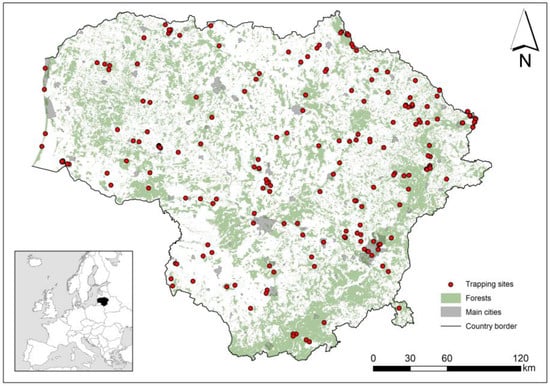
Figure 1.
Location of small mammal trapping sites in Lithuania, 1975–2023, with indication of forests, the main habitat of bank vole.
Habitat descriptions in the capture sites varied in categories and details, as there was no standard habitat classification used in small mammal studies in Lithuania. To be as compatible as possible with other small mammal studies, we categorized habitats into nine groups: agricultural, commensal, disturbed, forest, meadow, mixed, riparian, shrub, and wetland. This classification includes some of the CORINE level 3 habitats [48].
Arable land, fallow land, crops, complex cropping patterns, orchards, and berry plantations were included in the agricultural habitat group. Individual houses and yards, farmsteads, farms and their outbuildings, and industrial and commercial areas were considered commensal habitats for small mammals. Trappings in closed landfills and under-breeding colonies of Great Cormorants (Phalacrocorax carbo) were assigned to disturbed habitats and characterized by natural or anthropogenic disturbance. Forests included all types and ages of forest; this habitat group was the most variable. Grasslands included all grassland types (dry, wet and flooded, natural, seeded, and irrigated). All studied habitats, such as forests, shrubs, meadows, or wetlands within 50 m of the shoreline (island, lake, or river), were characterized as riparian. In the CORINE database, we characterized transitional forest–shrub as shrub habitats but also included shrubby meadows in this group. All wetland types, such as peat bogs, marshes, swamps, bogs, transitional wetlands, and reedbeds, were included in the wetland group. We further distinguished the case where a trap line covered several different habitats. These fragmented habitats, regardless of their composition, were characterized as mixed habitats.
2.2. Small Mammal Trapping and Sample Size
We analyzed material from small mammal trapping between 1975 and 2023. We used 7 × 14 cm wooden snap traps arranged in lines of 25 traps 5 m apart, with 1–12 lines per habitat. In a few trapping sessions, plastic or metal 7 × 14 cm snap traps or 5 × 10 cm metal traps were used. Traps were baited with brown bread and crude sunflower oil, set for three days, and checked once or twice a day, either in the morning or in the morning and evening. There were also cases where the traps stayed in place for 1–2 days, depending on the weather. The bait was replaced after rain or when it was absent for any reason. As indices based on line trapping have a tradition of more than 50 years in Lithuania, the results are directly comparable.
The total trapping effort was more than 500 thousand trap nights (Table 1). Equal trapping effort across decades was not ensured in the long term. However, the trapping effort and the number of individuals captured in each decade were sufficient to ensure the representation of all species and their diversity. Individual rarefaction shows that the threshold of about 500 trapped individuals ensures 13–14 small mammal species in the sample, and for characterization of diversity, it is sufficient to trap about 300 individuals (Figure S1). Even in the 2020s, with three years of trapping, this threshold was exceeded at least 6 times.

Table 1.
Trapping effort (TE, trap-days) and number of trapped specimens (N) according to decade.
Equal trapping effort across habitats was also not ensured (Table 2), but the minimum sample size of 352 trapped individuals in shrub habitats was sufficient to record at least 10 small mammal species (Figure S2). Therefore, the trappability of the dominant C. glareolus did not suffer.
Table 2.
Trapping effort (TE, trap-days) and number of trapped specimens (N) according to habitat: Agr—agricultural, Com—commensal, Dis—disturbed, For—forest, Mea—meadow, Mix—mixed, Rip—riparian, Shr—shrub, Wet—wetland habitats.
2.3. Data Analyses
Relative abundance (RA) of C. glareolus and all small mammal species as a whole was expressed per trap-day by dividing the number of individuals captured by the number of trap days. Proportions of C. glareolus in the small mammal community were expressed as percentages.
We tested these two variables, the relative abundance of C. glareolus and the species proportion in the small mammal community, for normality. Both variables were not normally distributed. The distribution of the relative abundance of C. glareolus was best approximated by a gamma function (Kolmogorov–Smirnov d = 0.0265, df = 5, NS).
Based on this function, two GLM analyses were conducted with decade, season, and habitat as categorical factors and trapping effort (number of trap days) and relative abundance of all small mammals as continuous predictors. The first model used the relative abundance of C. glareolus, and the second used the proportion of C. glareolus in the small mammal community as a dependent variable. Significance of factors was assessed using F and p, and effect size was assessed using partial eta-squared (η2). Graphical presentation was performed using mean and 95% confidence intervals (CI). The differences in dependent variables between categories of categorical factors were determined using post hoc analysis (Tukey HSD with unequal N). The minimum significance level was set at p < 0.05.
The consistency of the observed numbers of C. glareolus in different habitats with the expected numbers was tested using the χ2 statistic. We formulated the hypothesis H0 that the distribution of the number of individuals is independent of the habitat type and depends only on the trapping effort, while H1 was that the distribution of the number of individuals of C. glareolus is dependent on the habitat type, i.e., in some habitats, the observed number of trapped individuals exceeded that expected from the trapping effort. The null hypothesis is rejected at p < 0.05. Individual rarefaction was also used to test whether differences in C. glareolus numbers were influenced by sample size in different habitats.
The cyclicity of C. glareolus’s relative abundance was assessed visually from the plot of annual averages and confirmed by autocorrelation analysis.
Chi-square, test for normality of BCI distribution, and autocorrelation were calculated using PAST version 4.13 (Museum of Paleontology, Oslo College, Oslo, Norway) [49]. All other calculations were performed using Statistica for Windows, version 6.0 (StatSoft, Inc., Tulsa, OK, USA) [50].
3. Results
The first model explained 57% of C. glareolus RA and was significant (F = 111.7, df = 22, p < 0.0001). All factors except for trapping effort were significant. The strongest was the RA of all small mammals (F = 1359.6, p < 0.0001, η2 = 0.43), followed by the habitat (F = 31.2, p < 0.0001, η2 = 0.12). Temporal factors were much weaker, although both significant: decade (F = 9.2, p < 0.0001, η2 = 0.025) and season (F = 4.6, p < 0.0001, η2 = 0.018).
The second model explained 35% of the proportion of C. glareolus in small mammal communities. The most important factor was the habitat (F = 85.9, p < 0.0001, η2 = 0.28). The influence of the decade (F = 11.1, p < 0.0001, η2 = 0.03) and RA of all small mammals (F = 23.6, p < 0.0001, η2 = 0.013) was both highly significant but weak. The influence of the trapping effort (F = 0.0001, NS) and season (F = 1.2, NS) was not significant.
In both models, partial eta-squared showed the relative importance of different factors in a multivariate context by measuring the effect size for a particular factor after controlling for other variables in the model.
3.1. Main Habitats of Bank Vole in Lithuania
To remove the influence of trapping effort on the number of C. glareolus individuals retained, we calculated the expected catches from the data in Table 2 and compared them with the observed ones.
The number of C. glareolus captured in each habitat was significantly different from the predicted number (χ2 = 18,046, df = 8, p < 0.0001). The number of C. glareolus captured was 1.54 times higher than expected in forest habitats, 1.52 times higher in riparian habitats, and 1.47 times higher in mixed habitats. These habitats are the most important for C. glareolus in Lithuania. In disturbed, commensal, and shrub habitats, the number of captured C. glareolus differed from the expected number by 0.96–1.20 times, i.e., these habitats are neutral. Finally, the least important habitats for C. glareolus were meadows (the number of captured individuals was 4.17 times less than expected), agricultural areas (3.71 times less), and wetlands (the number of captured voles was 1.34 times less than expected). It should be noted that the best habitats are forested, while the worst are open. The presence of C. glareolus in commensal habitats requires further investigation.
3.2. Habitat Influence on C. glareolus Relative Abundance and Proportion
The average relative abundance of C. glareolus in Lithuania, regardless of season and habitat, was 0.036 ± 0.001 individuals per trap-day (Table 3).
Table 3.
Relative abundances (individuals per trap-day) and proportions (% of total number of individuals) of C. glareolus in the small mammal community according to habitats. TS—number of trapping sessions.
Based on the post hoc tests, we identified three habitat complexes with different relative abundances of C. glareolus. The highest RA, 0.042–0.061 ind./trap-day, was found in mixed, forest, riparian, disturbed, shrub, and commensal habitats. The mean RA was characteristic of wetlands. The lowest RA of C. glareolus, 0.012–0.014 ind./trap-day, was found in meadows and agricultural habitats. Thus, all the habitats with the highest RA except for commensal and shrubs are forested, and those with the lowest RA are open (Table 3).
As shown by the GLM, habitat had a significant influence on the relative abundance of C. glareolus (Figure S3A) and on the proportion of this species in the small mammal community (Figure S3B) when all other covariates were evaluated. Taking into account the long-term and seasonal dynamics, the highest RA of the species was in the wooded habitats, with the maximum in forests, and the lowest RA was in open agricultural habitats and meadows.
The average proportion of C. glareolus in small mammal communities, regardless of habitat, was 34 ± 0.9%, with the highest proportion in forests and the lowest in agricultural habitats (Table 3). Taking into account covariates (Figure S3B), the group of habitats with the highest proportion of the species includes forests, shrubs, and disturbed habitats (46.7–60.0%); the medium proportion is characteristic of commensal habitats, wetlands, mixed habitats, and riparian habitats; and the smallest proportion of the species was found in open agricultural habitats and meadows.
Local variability was very high because, in each habitat, there were trapping sessions where C. glareolus was absent and others where only bank voles were trapped.
3.3. Seasonal and Monthly Changes in C. glareolus Relative Abundance and Proportion
Seasonal changes indicate an upward trend in C. glareolus RA from a minimum in spring to winter, with abundance doubling by summer and being five times higher in fall and winter (Table 4). Long-term and habitat covariates did not alter this trend (Figure S4A). According to the post hoc, RA in fall and winter are similar, but other differences between seasons are significant. The proportion of C. glareolus remained constant in all seasons (Table 4, Figure S4B).
Table 4.
Relative abundances (individuals per trap-day) and proportions (% of total number of individuals) of C. glareolus in the small mammal community by season. TS—number of trapping sessions.
The monthly trend in RA of C. glareolus shows maximum values in November and December, then a steady ninefold decrease until April (Table 5). This minimum RA was found to last until June, doubled in July, and remained similar until November. The same dynamics were found when accounting for the influence of season and habitat covariates (Figure S5). Monthly changes in C. glareolus abundance did not show a regular pattern and were characterized by high variability between trapping sessions (Table 5).
Table 5.
Monthly relative abundances (individuals per trap-day) and proportions (% of total number of individuals) of C. glareolus in the small mammal community. TS—number of trapping sessions.
3.4. Long-Term Changes in C. glareolus Relative Abundance and Proportion
Long-term trends in RA of C. glareolus and species proportions in the small mammal community both decreased (Table 6). Post hoc analysis shows that the decrease in RA of C. glareolus in the 1980s (p < 0.02), 2010s (p < 0.05), and 2020s (p < 0.02) is significant compared to the 1970s, as well as the decrease in RA in the 2010s and 2020s compared to the 1990s and 2000s (all p < 0.01). Compared to the 1990s, the RA of C. glareolus was two times lower in the 2020s. The same trend was observed when controlling for season and habitat covariates (Figure S6A).
Table 6.
Relative abundances (individuals per trap-day) and proportions (% of total number of individuals) of C. glareolus in the small mammal community, independent of habitat, and in the forest habitat by decade. TS—number of trapping sessions.
Three periods of two decades were identified by analyzing the proportion of C. glareolus in small mammal communities. The highest proportion of the species, over 40%, was observed in the 1970s–1980s; the middle proportion, about 35%, was characteristic of the 1990s–2000s and decreased to about 20% in the 2010s–2020s (Table 6). According to the post hoc, the difference in proportion between the 1980s and 1990s is significant at p < 0.02, and all others at p < 0.001, while within the three periods, there were no significant differences. The decrease in C. glareolus proportions was significant after accounting for habitat and seasonal covariates (Figure S6B). We also compared C. glareolus proportions in forest habitats only and obtained the same significant trend; proportions decreased from approximately 70% to 46.4% in the 2010s and further to 36.4% in the 2020s (Figure S6C).
To test whether there were cyclic changes in the abundance of C. glareolus and all small mammal species, we analyzed trends in relative abundance in the fall, regardless of habitat, and in the forest habitat. Visual inspection showed no regular cycles in both the RA of C. glareolus (Figure 2A) and the small mammal community (Figure 2B) in all habitats, as well as no regular cycles in forests (Figure 3A,B). In forest habitats, variations in RA of C. glareolus were not pronounced, and CI overlapped. The absence of cycles was confirmed by autocorrelation analysis (Figure S7).
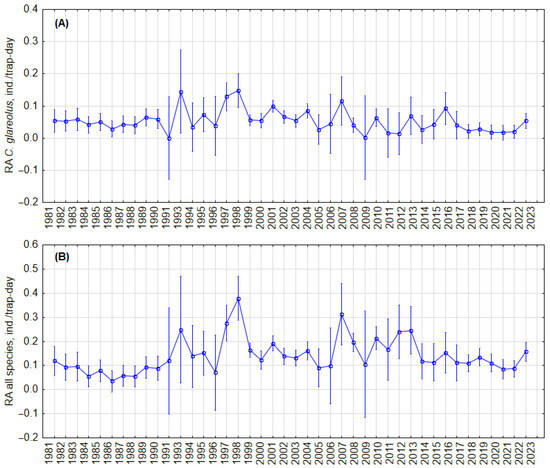
Figure 2.
Dynamics of the annual relative abundance of C. glareolus (A) and total relative abundance of all small mammal species (B) in autumn, independent of habitat. Vertical bars denote 95% CIs.
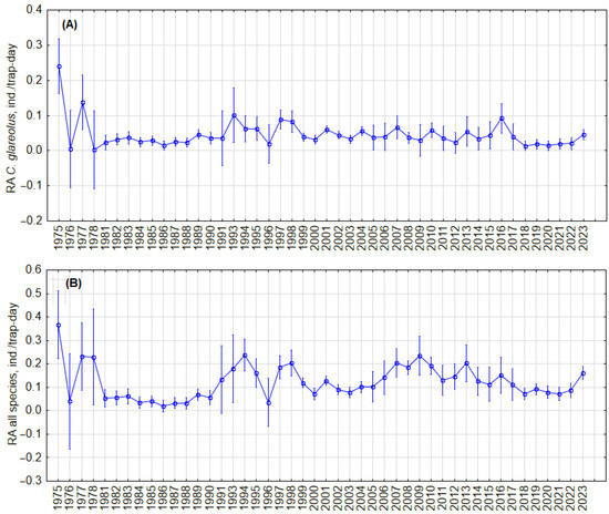
Figure 3.
Dynamics of the annual relative abundance of C. glareolus (A) and total relative abundance of all small mammal species (B) in autumn in forest habitat. Vertical bars denote 95% CIs.
4. Discussion
Our main findings relate to (1) the distribution of C. glareolus numbers in multiple habitats, identifying the most attractive for this species; (2) habitat-based differences in relative abundances and species proportions of C. glareolus in small mammal communities; and (3) temporal changes in these two parameters. These results are further discussed in the context of the species’ distribution in Europe.
4.1. Bank Vole Habitat Preferences
We found that habitat was the main factor explaining C. glareolus numbers in Lithuania, with the most preferred being wooded habitats—forests, riparian, and mixed habitats, the last two including forest fragments. The numbers of C. glareolus in open habitats, such as meadows, agricultural areas, and wetlands, were lower than expected according to the trapping effort. Our previous study documented an increase in C. glareolus numbers in succession from meadow to forest [39], in accordance with the general picture.
The above is fully consistent with the general characterization of C. glareolus as a woodland species [8,10]. In agricultural landscapes in the southern range of the species, this vole is associated with woodland patches [51]. The species was not found in grasslands, alfalfa, and maize crops when forest patches were present [52]. Further north, a multi-habitat study also characterized C. glareolus as absent in crops, avoiding grasslands and preferring mature and middle-aged forests [35]. Therefore, the number of C. glareolus in agricultural areas of Lithuania [12], and especially the number of this species in commensal habitats, coupled with their diet [53] and good body condition [42], requires further attention. Additional data should include a south–north gradient.
It should be noted that the absolute majority of the cited studies did not focus on microhabitat details. It is known that C. glareolus prefers dense forest cover [5]. However, although the thickness of fine litter was very important for C. glareolus, “the choice of microhabitat parameters is subordinate to that of macro-habitat characteristics, mainly tree and shrub cover” [51]. In general, fine-grained habitat inventory is not carried out in small mammal trapping, so very few studies really consider litter parameters or understorey complexity [54]. As a positive factor, the presence and density of undergrowth are mentioned [55,56], or, finally, the roughness of the undergrowth as a derived measure was shown to have a positive influence on the capture probability of C. glareolus [54].
4.2. South–North Cline in Bank Vole Proportion in Forests
We found that C. glareolus was generally the most abundant small mammal species in Lithuania, with an average proportion of 34.0% in small mammal communities. In the forest and other wooded habitats, these proportions ranged from 46.7% to the highest of 60.0% in forests.
The proportion of C. glareolus in forest habitats fits into a broader picture covering different European countries (Table 7). Although the presented dataset covers a long period of time and is not designed to compare long-term trends, it is clear that the representation of C. glareolus in forest small mammal communities follows a geographical gradient, increasing from south to north. In the northernmost area, the species is absolutely dominant in late successional forests [26]. It should be noted that such comparisons have drawbacks and uncertainties, as the habitat is not adequately described (see the footnotes of Table 7). Thus, while the decline in C. glareolus in small mammal communities can be predicted from the articles of different authors, the concept of the cline itself has not been applied so far. We consider this to be one of the most important results of this study.
Table 7.
Proportion of C. glareolus in forests from countries of different latitudes. A. fla—A. flavicollis, % Dom.—dominant species and its proportion in small mammal community, % C. gla.—proportion of C. glareolus in small mammal community.
Similar to the relative abundance, the proportions of C. glareolus found in open habitats (8.6% in agricultural areas and 11.9% in meadows) are consistent with the neighboring region. In Latvia, the species was not recorded in grasslands [63], 0 to 6–15% in grasslands of Poland [61], and 4% in meadows [36], while in grasslands of Estonia, this proportion was 26.9% [35]. The last two figures are not based on a long time period.
4.3. Relative Abundance of Bank Vole Is Typical to the Region
Comparisons of relative abundances require more in-depth analysis because (1) it is not clear in which phase of population change the survey was conducted over a short period of time, (2) it is not always clear whether trapping methods had an influence (e.g., type of trap, trap placement, bait, frequency of control, etc.), and (3) the habitats are not all described in the same way, and according to our results, the differences between RAs between the two habitats are apparent.
In Lithuania, the mean relative abundance of C. glareolus, independent of season and habitat, was 0.036 individuals per trap-day, 0.059 individuals per trap-day in the forest, with a maximum of 0.533 individuals per trap-day. These numbers are in line with many other countries. In neighboring Latvia, the average RA was 0.056, and 0.064 ind./trap-day in mixed forests [63].
South of Lithuania, in Poland, the mean RA of C. glareolus in seven large forests ranged from 0.037 to 0.085 ind./trap-day. It was positively related to the proportion of deciduous stands, which was 29.7% and 82.4%, respectively [62]. Further south, in deciduous stands of Germany, RA is reported to be between 0.02 and 0.20 ind./trap-day [37]. These values correspond to the long-term variation of C. glareolus in Germany, which was in the range of 0.01–0.18 during 1950–2010 [38]. In the oak forest of Bulgaria, the RA of C. glareolus was 0.069 ind./trap-day [52].
North of Lithuania, in Sweden, the relative abundance of the species in 1970–2015 ranged from 0 to 0.013 ind./trap-day and fluctuated markedly, with 12 distinct cycles in the mentioned period [29], but with no general average data from the authors. Further north, the average RA was 0.067, with a maximum of 0.20 ind./trap-day [66]. In the northernmost study, in Finnish Lapland, the annual relative abundance of C. glareolus varied from zero to 0.30 ind./trap-day in 1970–2000 [25].
4.4. Short- and Long-Term Changes in Population Indices of C. glareolus
We observed monthly and seasonal differences of RA in C. glareolus (see Table 4 and Table 5), which remain valid, taking into account the influence of long-term and habitat covariates. Maximum RA was observed in November and December, then decreased until April and remained at a minimum until July. An increase in RA from May to mid-July was reported by M. Mazurkiewicz [67] or from April to October by A. Bajer et al. [68], both in similar latitudes; however, these authors, as most of the others, do not catch small mammals in the non-vegetation period. References confirming this statement can be found in [66,69]. Therefore, our data on monthly changes in C. glareolus RA are sufficiently original not only for the country but also regionally. Seasonal changes of RA, with an upward trend from minimum in spring to winter, only confirm the monthly dynamics on a coarser scale.
Our results did not show a regular pattern of monthly changes in C. glareolus proportions (see Table 5), but they were constant in all seasons (Table 4, Figure S4B). Again, most of the cited authors compare only two seasons, spring and fall [66,70], sometimes three, including summer [55,61,67], but rarely in winter [69].
We did not find cyclic changes in the relative abundance of C. glareolus in general, regardless of habitat, nor in the forest habitat. Visually, two periods can be observed: 1981–1990 and 2017–2023, both marked by relatively low and stable densities of C. glareolus, and 1991–2016, characterized by higher but fluctuating densities independent of habitat, as illustrated in Figure 2. Similar patterns are noted in forest habitats (Figure 3). Despite these fluctuations, the long-term trend for C. glareolus is decreasing and non-cyclic, as shown in Figures S6 and S7. The absence of abundance cycles of this species fits into a more general picture—cyclic fluctuations in the northern part of the range [15,23,24,31,71], absence or dampening of RA fluctuations in Latvia and Estonia [34,35,63], and irregular outbreaks in the south [36,37,61]. The alternation of low and high abundance, as well as outbreaks, are related to summer temperatures and masting [38]. In the current study, we do not analyze weather parameters and food of voles, focusing only on the picture of population changes.
The other strong finding of this study is the decreasing long-term trend in both RA of C. glareolus and species proportions in the small mammal community (see Table 6). Compared to the 1990s, RA was two times lower in the 2020s, and accounting for the covariates of season and habitat did not change the trend (see Figure S6A). In terms of proportion, there were three periods of decreasing C. glareolus proportion in the small mammal community: the species comprised over 40% in the 1970s–1980s, about 35% in the 1990s–2000s, about 20% in the 2010s–2020s, and these differences were significant after accounting for covariates of habitat and season (see Figure S6B). In the forest habitat, the proportion of C. glareolus almost halved during the whole period (see Figure S6C).
A decreasing proportion of C. glareolus was observed in Latvia after the 1990s [63]. According to the data presented in [61], the proportions of the species in two different habitats in Poland remained stable. Long-term trends of C. glareolus proportions in Fennoscandian studies are not clear, but based on abundance data, proportions are highest in remnant semi-natural old-growth forests compared to not only middle-aged stands but also older cultivated stands [65].
There are also marker differences in the temporal synchrony of RA changes in different small mammal species, with interspecific synchrony not observed in Latvia [34,63] and Lithuania [40]. However, this is characteristic of small mammal communities in the north [72]. These differences may be related to differences in the postglacial history of the species. Based on dispersal from different glacial refugia, C. glareolus populations in Lithuania, Latvia, and Poland are a mix of Carpathian and Eastern lineages [73]. These lineages differ not only in their ecological niche requirements but also phenotypically [74]. However, there is no way to genetically test processed individuals, as our data are all retrospective.
The reciprocal relationship between dominance and diversity in communities is a well-known phenomenon [75,76], and it is not only for small mammals [77]. As shown in the example of a flooded meadow in Lithuania, the absence of small mammals in the post-flood area allows non-dominant species to reach high relative abundances [40]. A decrease in the diversity of the small mammal community in Sweden was related to an increase in the proportion of C. glareolus [29]. And vice versa, we related the increase in small mammal diversity in Lithuania to a decrease in dominance in their community, which in turn was related to a decrease in the proportion of C. glareolus [41].
5. Conclusions
According to the proportion of this species in forest small mammal communities, C. glareolus in Lithuania is in the middle of a south–north increasing cline. On the basis of long-term trapping data, we found that C. glareolus is not cyclic and is decreasing in proportion and in relative abundance. The increasing diversity of small mammals in the country in recent decades can be attributed to these changes.
Supplementary Materials
The following supporting information can be downloaded at: https://www.mdpi.com/article/10.3390/d16090546/s1, Figure S1: Accumulation curves of species (A) and diversity (B) of the small mammal community in relation to the number of specimens trapped in different decades; Figure S2: Accumulation curves of species (A) and diversity (B) of the small mammal community in relation to the number of specimens trapped in different habitats; Figure S3: Habitat effect of relative abundance (A) and proportion of C. glareolus in the small mammal community (B), calculated by evaluating covariates at their means. Vertical bars denote 95% CI; Figure S4: Seasonal changes in relative abundance (A) and proportion of C. glareolus in the small mammal community (B), calculated by evaluating covariates at their means. Vertical bars denote 95% CI; Figure S5: Monthly changes of the relative abundance of C. glareolus, calculated by evaluating co-variates at their means. Vertical bars denote 95% CI; Figure S6: Long-term changes in relative abundance (A), the proportion of C. glareolus in the small mammal community in all habitats (B) and in the forest habitat (C), calculated by evaluating the covariates at their means. Vertical bars denote 95% CI; Figure S7: Autocorrelation of annual relative abundances of C. glareolus in autumn in forest habitats with different lag periods.
Author Contributions
Conceptualization, L.B. (Linas Balčiauskas); investigation, all authors; formal analysis, L.B. (Linas Balčiauskas); writing—original draft preparation, all authors; writing—review and editing, all authors. All authors have read and agreed to the published version of the manuscript.
Funding
The work of the authors was funded by the Nature Research Centre budget.
Institutional Review Board Statement
This study uses historical material on small mammal trapping and material collected for other projects. It was conducted in accordance with Lithuanian legislation (the Republic of Lithuania Law on the Welfare and Protection of Animals No. XI-2271, “Requirements for the Housing, Care and Use of Animals for Scientific and Educational Purposes”, approved by Order No B1-866, 31 October 2012 of the Director of the State Food and Veterinary Service (Paragraph 4 of Article 16) and European legislation (Directive 2010/63/EU) on the protection of animals and was approved by the Animal Welfare Committee of the Nature Research Centre, protocol No. GGT-7 and GGT-8).
Data Availability Statement
This is ongoing research; therefore, data are available from the corresponding author upon reasonable request.
Acknowledgments
We acknowledge A. Kučas for providing a map of the trapping sites. The authors are grateful to all former colleagues and staff members of the Regional Parks who participated in the monitoring of small mammals.
Conflicts of Interest
The authors declare no conflicts of interest.
References
- Moritz, C.; Patton, J.L.; Conroy, C.J.; Parra, J.L.; White, G.C.; Beissinger, S.R. Impact of a century of climate change on small-mammal communities in Yosemite National Park, USA. Science 2008, 322, 261–264. [Google Scholar] [CrossRef]
- Auffray, J.C.; Renaud, S.; Claude, J. Rodent biodiversity in changing environments. Kasetsart J. Nat. Sci. 2009, 43, 83–93. [Google Scholar]
- Santoro, S.; Sanchez-Suarez, C.; Rouco, C.; Palomo, L.J.; Fernández, M.C.; Kufner, M.B.; Moreno, S. Long-term data from a small mammal community reveal loss of diversity and potential effects of local climate change. Curr. Zool. 2017, 63, 515–523. [Google Scholar] [CrossRef] [PubMed][Green Version]
- Balestrieri, A.; Gazzola, A.; Formenton, G.; Canova, L. Long-term impact of agricultural practices on the diversity of small mammal communities: A case study based on owl pellets. Environ. Monit. Assess. 2019, 191, 725. [Google Scholar] [CrossRef]
- Naeem, S.; Li, S. Biodiversity enhances ecosystem reliability. Nature 1997, 390, 507–509. [Google Scholar] [CrossRef]
- Tilman, D.; Reich, P.; Knops, J. Biodiversity and ecosystem stability in a decade-long grassland experiment. Nature 2006, 441, 629–632. [Google Scholar] [CrossRef] [PubMed]
- Avenant, N. The potential utility of rodents and other small mammals as indicators of ecosystem ‘integrity’of South African grasslands. Wildl. Res. 2011, 38, 626–639. [Google Scholar] [CrossRef]
- Hutterer, R.; Kryštufek, B.; Yigit, N.; Mitsainas, G.; Palomo, L.; Henttonen, H.; Vohralík, V.; Zagorodnyuk, I.; Juškaitis, R.; Meinig, H.; et al. Myodes glareolus. In The IUCN Red List of Threatened Species 2021: E.T4973A197520967; IUCN: Gland, Switzerland, 2021. [Google Scholar] [CrossRef]
- Viro, P.; Niethammer, J. Clethrionomys glareolus (Schreber, 1780)—Rötelmaus. In Handbuch der Säugetiere Europas, Band 2/I: Nagetiere II; Niethammer, J., Krapp, F., Eds.; Akademische Verlagsgesellschaft: Wiesbaden, Germany, 1982; pp. 109–140. [Google Scholar]
- Spitzenberger, F. Clethrionomys glareolus. In The Atlas of European Mammals; Mitchell-Jones, A.J., Amori, G., Bogdanowicz, W., Kryštufek, B., Reijnders, P.J.H., Spitzenberger, F., Stubbe, M., Thissen, J.B.M., Vohralík, V., et al., Eds.; Academic Press: London, UK, 1999; pp. 201–211. [Google Scholar]
- Butet, A.; Delettre, Y.R. Diet differentiation between European arvicoline and murine rodents. Acta Theriol. 2011, 56, 297–304. [Google Scholar] [CrossRef]
- Balčiauskas, L.; Stirkė, V.; Garbaras, A.; Skipitytė, R.; Balčiauskienė, L. Stable Isotope Analysis Supports Omnivory in Bank Voles in Apple Orchards. Agriculture 2022, 12, 1308. [Google Scholar] [CrossRef]
- Prūsaitė, J. Fauna of Lithuania. Mammals; Mokslas: Vilnius, Lithuania, 1988; p. 295. [Google Scholar]
- Suchomel, J.; Šipoš, J.; Ouředníčková, J.; Skalský, M.; Heroldová, M. Bark Gnawing by Rodents in Orchards during the Growing Season—Can We Detect Relation with Forest Damages? Agronomy 2022, 12, 251. [Google Scholar] [CrossRef]
- Andreassen, H.P.; Sundell, J.; Ecke, F.; Halle, S.; Haapakoski, M.; Henttonen, H.; Huitu, O.; Jacob, J.; Johnsen, K.; Koskela, E.; et al. Population cycles and outbreaks of small rodents: Ten essential questions we still need to solve. Oecologia 2021, 195, 601–622. [Google Scholar] [CrossRef] [PubMed]
- Krebs, C.J.; Kenney, A.J.; Gilbert, B.S.; Boonstra, R. Long-term monitoring of cycles in Clethrionomys rutilus in the Yukon boreal forest. Integr. Zool. 2024, 19, 27–36. [Google Scholar] [CrossRef]
- Magnusson, M.; Hörnfeldt, B.; Ecke, F. Evidence for different drivers behind long-term decline and depression of density in cyclic voles. Popul. Ecol. 2015, 57, 569–580. [Google Scholar] [CrossRef]
- Ims, R.A.; Henden, J.A.; Killengreen, S.T. Collapsing Population Cycles. Trends Ecol. Evol. 2008, 23, 79–86. [Google Scholar] [CrossRef]
- Cornulier, T.; Yoccoz, N.G.; Bretagnolle, V.; Brommer, J.E.; Butet, A.; Ecke, F.; Elston, D.A.; Framstad, E.; Henttonen, H.; Hörnfeldt, B.; et al. Europe-Wide Dampening of Population Cycles in Keystone Herbivores. Science 2013, 340, 63–66. [Google Scholar] [CrossRef] [PubMed]
- Sundell, J.; Huitu, O.; Henttonen, H.; Kaikusalo, A.; Korpimäki, E.; Pietiäinen, H.; Saurola, P.; Hanski, I. Large-scale spatial dynamics of vole populations in Finland revealed by the breeding success of vole-eating predators. J. Anim. Ecol. 2004, 73, 167–178. [Google Scholar] [CrossRef]
- Brommer, J.E.; Pietiäinen, H.; Ahola, K.; Karell, P.; Karstinenz, T.; Kolunen, H. The Return of the Vole Cycle in Southern Finland Refutes the Generality of the Loss of Cycles through “Climatic Forcing”. Glob. Chang. Biol. 2010, 16, 577–586. [Google Scholar] [CrossRef]
- Kiseleva, N.V. Long-Term Monitoring of the Numbers of Forest Rodents in Ilmeny Reserve. Biol. Bull. Russ. Acad. Sci. 2021, 48, 1839–1842. [Google Scholar] [CrossRef]
- Bobretsov, A.V.; Lukyanova, L.E.; Bykhovets, N.M.; Petrov, A.N. Impact of climate change on population dynamics of forest voles (Myodes) in northern Pre-Urals: The role of landscape effects. Contemp. Probl. Ecol. 2017, 10, 215–223. [Google Scholar] [CrossRef]
- Ivanter, E.V. Toward the study of population dynamics of the bank vole (Myodes glareolus Schr.) at the northern periphery of its range [К изучению динамики численнoсти рыжей пoлевки (Myodes glareolus Schr.) на севернoй периферии ареала]. Proc. Karelian Sci. Cent. Russ. Acad. Sci. 2019, 11, 74–88. [Google Scholar]
- Henttonen, H. Long-term dynamics of the bank vole Clethrionomys glareolus at Pallasjärvi, Northern Finnish taiga. Pol. J. Ecol. 2000, 48, 87–96. [Google Scholar]
- Ecke, F.; Löfgren, O.; Sörlin, D. Population dynamics of small mammals in relation to forest age and structural habitat factors in northern Sweden. J. Appl. Ecol. 2002, 39, 781–792. [Google Scholar] [CrossRef]
- Andrén, H.; Liberg, O. Numerical response of predator to prey: Dynamic interactions and population cycles in Eurasian lynx and roe deer. Ecol. Monogr. 2024, 94, e1594. [Google Scholar] [CrossRef]
- Hörnfeldt, B. Long-Term Decline in Numbers of Cyclic Voles in Boreal Sweden: Analysis and Presentation of Hypotheses. Oikos 2004, 107, 376–392. [Google Scholar] [CrossRef]
- Ecke, F.; Angeler, D.G.; Magnusson, M.; Khalil, H.; Hörnfeldt, B. Dampening of population cycles in voles affects small mammal community structure, decreases diversity, and increases prevalence of a zoonotic disease. Ecol. Evol. 2017, 7, 5331–5342. [Google Scholar] [CrossRef] [PubMed]
- Oli, M.K. Population cycles in voles and lemmings: State of the science and future directions. Mammal Rev. 2019, 49, 226–239. [Google Scholar] [CrossRef]
- Soininen, E.M.; Neby, M. Small rodent population cycles and plants–after 70 years, where do we go? Biol. Rev. 2024, 99, 265–294. [Google Scholar] [CrossRef] [PubMed]
- Rammul, Ü.; Oksanen, T.; Oksanen, L.; Lehtelä, J.; Virtanen, R.; Olofsson, J.; Strengbom, J.; Rammul, I.; Ericson, L. Vole–vegetation interactions in an experimental, enemy free taiga floor system. Oikos 2007, 116, 1501–1513. [Google Scholar] [CrossRef]
- Massey, F.P.; Smith, M.J.; Lambin, X.; Hartley, S.E. Are silica defences in grasses driving vole population cycles? Biol. Lett. 2008, 4, 419–422. [Google Scholar] [CrossRef]
- Avotins, A.; Avotins, A., Sr.; Ķerus, V.; Aunins, A. Numerical Response of Owls to the Dampening of Small Mammal Population Cycles in Latvia. Life 2023, 13, 572. [Google Scholar] [CrossRef]
- Väli, Ü.; Tõnisalu, G. Community- and Species-Level Habitat Associations of Small Mammals in a Hemiboreal Forest-Farmland Landscape. Ann. Zool. Fenn. 2020, 58, 1–11. [Google Scholar] [CrossRef]
- Zub, K.; Jędrzejewska, B.; Jędrzejewski, W.; Barton, K.A. Cyclic voles and shrews and non-cyclic mice in a marginal grassland within European temperate forest. Acta Theriol. 2012, 57, 205–216. [Google Scholar] [CrossRef] [PubMed]
- Bujnoch, F.M.; Reil, D.; Drewes, S.; Rosenfeld, U.M.; Ulrich, R.G.; Jacob, J.; Imholt, C. Small mammal community composition impacts bank vole (Clethrionomys glareolus) population dynamics and associated seroprevalence of Puumala orthohantavirus. Integr. Zool. 2024, 19, 52–65. [Google Scholar] [CrossRef]
- Imholt, C.; Reil, D.; Eccard, J.A.; Jacob, D.; Hempelmann, N.; Jacob, J. Quantifying the past and future impact of climate on outbreak patterns of bank voles (Myodes glareolus). Pest Manag. Sci. 2015, 71, 166–172. [Google Scholar] [CrossRef] [PubMed]
- Balčiauskas, L.; Čepukienė, A.; Balčiauskienė, L. Small mammal community response to early meadow–forest succession. For. Ecosyst. 2017, 4, 11. [Google Scholar] [CrossRef]
- Balčiauskas, L.; Balčiauskienė, L. Long-term changes in a small mammal community in a temperate zone meadow subject to seasonal floods and habitat transformation. Integr. Zool. 2022, 17, 443–455. [Google Scholar] [CrossRef]
- Balčiauskas, L.; Balčiauskienė, L. Small Mammal Diversity Changes in a Baltic Country, 1975–2021: A Review. Life 2022, 12, 1887. [Google Scholar] [CrossRef]
- Balčiauskas, L.; Balčiauskienė, L. Insight into Body Condition Variability in Small Mammals. Animals 2024, 14, 1686. [Google Scholar] [CrossRef]
- Juknelienė, D.; Kazanavičiūtė, V.; Valčiukienė, J.; Atkocevičienė, V.; Mozgeris, G. Spatiotemporal Patterns of Land-Use Changes in Lithuania. Land 2021, 10, 619. [Google Scholar] [CrossRef]
- Lithuanian Statistical Yearbook. National Land Service under the Ministry of Agriculture of the Republic of Lithuania. Available online: http://www.nzt.lt/go.php/lit/Lietuvos-respublikos-zemes-fondas (accessed on 1 August 2024).
- Mozgeris, G.; Brukas, V.; Pivoriūnas, N.; Činga, G.; Makrickienė, E.; Byčenkienė, S.; Marozas, V.; Mikalajūnas, M.; Dudoitis, V.; Ulevičius, V.; et al. Spatial Pattern of Climate Change Effects on Lithuanian Forestry. Forests 2019, 10, 809. [Google Scholar] [CrossRef]
- Rowe, R.J.; Terry, R.C. Small mammal responses to environmental change: Integrating past and present dynamics. J. Mammal. 2014, 95, 1157–1174. [Google Scholar] [CrossRef]
- Brodie, J.F. Synergistic effects of climate change and agricultural land use on mammals. Front. Ecol. Environ. 2016, 14, 20–26. [Google Scholar] [CrossRef]
- CORINE Land Cover. Available online: https://land.copernicus.eu/pan-european/corine-land-cover (accessed on 12 May 2024).
- Past 4—The Past of the Future. Available online: https://www.nhm.uio.no/english/research/resources/past/ (accessed on 1 January 2024).
- TIBCO Software Inc. Data Science Textbook. Available online: https://docs.tibco.com/data-science/textbook (accessed on 15 January 2024).
- Balestrieri, A.; Remonti, L.; Morotti, L.; Saino, N.; Prigioni, C.; Guidali, F. Multilevel habitat preferences of Apodemus sylvaticus and Clethrionomys glareolus in an intensively cultivated agricultural landscape. Ethol. Ecol. Evol. 2015, 29, 38–53. [Google Scholar] [CrossRef]
- Metcheva, R.; Beltcheva, M.; Aleksieva, I.; Heredia-Rojas, J.A.; Ostoich, P. Species Composition and Population Structure of Rodent Communities in Different Habitats in the Lozenska Mountain, Bulgaria. Acta Zool. Bulgar. 2020, (Suppl. S15), 205–209. [Google Scholar]
- Balčiauskas, L.; Balčiauskienė, L.; Garbaras, A.; Stirkė, V. Diversity and Diet Differences of Small Mammals in Commensal Habitats. Diversity 2021, 13, 346. [Google Scholar] [CrossRef]
- Appleby, S.M.; Bebre, I.; Riebl, H.; Balkenhol, N.; Seidel, D. Linking small mammal capture probability with understory structural complexity using a mobile laser scanning-derived metric: A case study. Ecol. Res. 2024, 39, 360–367. [Google Scholar] [CrossRef]
- Lešo, P.; Lešová, A.; Kropil, R.; Kaňuch, P. Response of the dominant rodent species to close-to-nature logging practices in a temperate mixed forest. Ann. For. Res. 2016, 59, 259–268. [Google Scholar] [CrossRef]
- Čepelka, L.; Purchart, L.; Suchomel, J. Small Mammal Community of Forest Stands in Drahanská vrchovina Upland (Czech Republic). Beskydy 2016, 8, 91–100. [Google Scholar] [CrossRef]
- Torre, I.; Arrizabalaga, A. Habitat preferences of the bank vole Myodes glareolus in a Mediterranean mountain range. Acta Theriol. 2008, 53, 241–250. [Google Scholar] [CrossRef]
- Benedek, A.M.; Sîrbu, I.; Lazăr, A. Responses of small mammals to habitat characteristics in Southern Carpathian forests. Sci. Rep. 2021, 11, 12031. [Google Scholar] [CrossRef]
- Lazăr, A.; Benedek, A.M.; Sîrbu, I. Small Mammals in Forests of Romania: Habitat Type Use and Additive Diversity Partitioning. Forests 2021, 12, 1107. [Google Scholar] [CrossRef]
- Suchomel, J.; Šipoš, J.; Košulič, O. Management Intensity and Forest Successional Stages as Significant Determinants of Small Mammal Communities in a Lowland Floodplain Forest. Forests 2020, 11, 1320. [Google Scholar] [CrossRef]
- Kozakiewicz, M.; Kozakiewicz, A. Long-term dynamics and biodiversity changes in small mammal communities in a mosaic of agricultural and forest habitats. Ann. Zool. Fenn. 2008, 45, 263–269. [Google Scholar] [CrossRef]
- Niedziałkowska, M.; Kończak, J.; Czarnomska, S.; Jędrzejewska, B. Species diversity and abundance of small mammals in relation to forest productivity in northeast Poland. Écoscience 2010, 17, 109–119. [Google Scholar] [CrossRef]
- Pupila, A.; Bergmanis, U. Species diversity, abundance and dynamics of small mammals in the Eastern Latvia. Acta Univ. Latv. 2006, 710, 93–101. [Google Scholar]
- Schlinkert, H.; Ludwig, M.; Batáry, P.; Holzschuh, A.; Kovács-Hostyánszki, A.; Tscharntke, T.; Fischer, C. Forest specialist and generalist small mammals in forest edges and Hedges. Wildl. Biol. 2016, 22, 86–94. [Google Scholar] [CrossRef]
- Wegge, P.; Rolstad, J. Cyclic small rodents in boreal forests and the effects of even-aged forest management: Patterns and predictions from a long-term study in southeastern Norway. For. Ecol. Manag. 2018, 422, 79–86. [Google Scholar] [CrossRef]
- Savola, S.; Henttonen, H.; Lindén, H. Vole population dynamics during the succession of a commercial forest in northern Finland. Ann. Zool. Fenn. 2013, 50, 79–88. [Google Scholar] [CrossRef]
- Mazurkiewicz, M. Population dynamics and demography of the bank vole in different tree stands. Acta Theriol. 1991, 36, 207–227. [Google Scholar] [CrossRef]
- Bajer, A.; Behnke, J.M.; Pawełczyk, A.; Kuliś, K.; Sereda, M.J.; Siński, E. Medium-term temporal stability of the helminth component community structure in bank voles (Clethrionomys glareolus) from the Mazury Lake District region of Poland. Parasitology 2005, 130, 213–228. [Google Scholar] [CrossRef]
- Crespin, L.; Verhagen, R.; Stenseth, N.C.; Yoccoz, N.G.; Prévot-Julliard, A.C.; Lebreton, J.D. Survival in fluctuating bank vole populations: Seasonal and yearly variations. Oikos 2002, 98, 467–479. [Google Scholar] [CrossRef]
- Steen, H.; Ims, R.A.; Sonerud, G.A.; Ecology, S.; Dec, N. Spatial and Temporal Patterns of Small-Rodent Population Dynamics at a Regional Scale. Ecology 1996, 77, 2365–2372. [Google Scholar] [CrossRef]
- Sørensen, O.J.; Moa, P.F.; Hagen, B.R.; Selås, V. Possible impact of winter conditions and summer temperature on bank vole (Myodes glareolus) population fluctuations in Central Norway. Ethol. Ecol. Evol. 2023, 35, 471–487. [Google Scholar] [CrossRef]
- Korpimaki, E.; Norrdahl, K.; Huitu, O.; Klemola, T. Predator-induced synchrony in population oscillation s of coexisting small mammal species. Proc. R. Soc. Sect. B 2005, 272, 193–202. [Google Scholar] [CrossRef]
- Escalante, M.A.; Horníková, M.; Marková, S.; Kotlík, P. Niche differentiation in a postglacial colonizer, the bank vole Clethrionomys glareolus. Ecol. Evol. 2021, 11, 8054–8070. [Google Scholar] [CrossRef]
- Ledevin, R.; Michaux, J.R.; Deffontaine, V.; Henttonen, H.; Renaud, S. Evolutionary history of the bank vole Myodes glareolus: A morphometric perspective. Biol. J. Linn. Soc. 2010, 100, 681–694. [Google Scholar] [CrossRef]
- Thukral, A.K.; Bhardwaj, R.; Kumar, V.; Sharma, A. New indices regarding the dominance and diversity of communities, derived from sample variance and standard deviation. Heliyon 2019, 5, E02606. [Google Scholar] [CrossRef] [PubMed]
- Martin, C.A.; Watson, C.J.; de Grandpré, A.; Desrochers, L.; Deschamps, L.; Giacomazzo, M.; Loiselle, A.; Paquette, C.; Pépino, M.; Rainville, V.; et al. The dominance–diversity dilemma in animal conservation biology. PLoS ONE 2023, 18, e0283439. [Google Scholar] [CrossRef]
- de la Peña, N.M.; Butet, A.; Delettre, Y.; Paillat, G.; Morant, P.; Le Du, L.; Burel, F. Response of the small mammal community to changes in western French agricultural landscapes. Landsc. Ecol. 2003, 18, 265–278. [Google Scholar] [CrossRef]


Disclaimer/Publisher’s Note: The statements, opinions and data contained in all publications are solely those of the individual author(s) and contributor(s) and not of MDPI and/or the editor(s). MDPI and/or the editor(s) disclaim responsibility for any injury to people or property resulting from any ideas, methods, instructions or products referred to in the content. |
© 2024 by the authors. Licensee MDPI, Basel, Switzerland. This article is an open access article distributed under the terms and conditions of the Creative Commons Attribution (CC BY) license (https://creativecommons.org/licenses/by/4.0/).