Spatiotemporal Variations in Phytoplankton Community Structure and Diversity: A Case Study for a Macroalgae–Oyster Reef Ecosystem

Abstract

The estuarine area of Luanhe River is an important fisheries ground in China’s Bohai Sea. In 2016, Tangshan Marine Ranching Co., Ltd. constructed a 2 km² artificial oyster–macroalgae reef area by placing artificial reefs on the seabed adjacent to the Luanhe River Estuary. This action resulted in sustainable annual economic outputs through the fishing and sea cucumber put-and-take fishery. Although Luanhe River runoff and reef construction are important to the local phytoplankton community and fisheries’ production, little is known about how these factors affect phytoplankton community structure in the local coastal ecosystem. In this study, we conducted field surveys to investigate the spatiotemporal variations in species composition, abundance, dominant species, diversity indexes, niche width and overlap, and interspecific connection of the phytoplankton community in the ecosystem of oyster–macroalgal reefs. From July 2016 to August 2017, we collected data before and after reef construction in areas inside and outside of the benthic reefs in both the flood and dry seasons of Luanhe River runoff. We found a total of 79 species, with the majority represented by diatoms and dinoflagellates. The dominant species were Paralia sulcata and Coscinodiscus sp. The total species number and abundance increased from May to September. The species number in the reef area was greater than that outside the reef. Species abundance from August to September was greater in the reef area than in the control area, which was opposite the situation from May to June. We found more phytoplankton abundance in the flood season compared with that in the dry season. Our results suggest that reef construction can benefit the local phytoplankton community and that further studies of the relationship among oysters, macroalgae, and phytoplankton in the system are warranted. Moreover, we provide baseline data about variations in the phytoplankton community in a sea ranch area.

1. Introduction

Marine phytoplankton are distributed widely across continental shelves, including the coastal temperate productive areas of oyster and macroalgal reefs [1]. They are a diverse set of critical primary producers that form the base of the marine ecosystem, and they are an important food source for a diverse array of predators, including benthic suspension feeders such as Pacific oysters (Crassostrea gigas) [2]. Phytoplankton play a fundamental role in improving the productivity of the entire coastal ecosystem and likely benefit fisheries’ production and ecosystem function coastal sea ranch areas [3]. Many reports of coastal phytoplankton production and distribution at shelf-wide and broader oceanographic scales exist [4,5,6], but fewer studies have focused on variations in the species composition, diversity, and abundance of phytoplankton in coastal rocky reefs of shallow subtidal zones. The estuarine area of Luanhe River is a historically important fisheries ground within Bohai Bay in China’s Bohai Sea [7,8,9]. In 2016, the local fisheries community in this area constructed a 2 km² artificial reef area by placing concrete on the seabed. These artificial reefs developed into oyster–macroalgae reefs because the native macroalgae (Sargassum muticum, Sargassum thunbergii, and Ulva lactuca) and oysters (C. gigas) naturally colonized the hard substrate [8].

In a previous study, we found that phytoplankton and macroalgae were the primary producers in the system, and phytoplankton biomass values were lowest in summer [7]. The greater concentration of phytoplankton biomass at the sea bottom might be related to the existence of the artificial reefs compared with the sea surface [10]. Oysters such as C. gigas can assert both top-down and bottom-up control via active filter feeding and biodeposition [11,12]. Macroalgae can decrease the amount of marine phytoplankton by creating unfavorable light conditions, thereby decreasing the net primary productivity of the local system [1]. In this system, benthic macroalgae and marine pelagic phytoplankton are the autotrophs and net primary producers, and the suspended-filter feeding oyster C. gigas is a secondary producer. Thus, this is an optimal habitat pattern for exploring the variations in marine phytoplankton community structure and abundance in a coastal reef ecosystem, with the further goal of understanding the variation in the structure and function of the ecosystem. Moreover, China’s Bohai Bay is a semi-closed basin that receives inflow from the Luanhe River. The Luanhe River runs off the mountain area at Qianʹan and brings abundant nutrients for estuarine organisms [13,14]. Thus, we explored the spatiotemporal variations in the phytoplankton community in a case of reef construction and Luanhe River runoff in a small sea ranch area.

In the marine phytoplankton community of the Bohai Sea, the proportion of dinoflagellates to diatoms has been increasing and the size of individuals has been decreasing since the 2000s [15]. The dominant species of diatoms has changed from the larger-celled Chaetoceros spp. and Coscinodiscus spp. to nano-celled Paralia sulcata and Thalassionema spp. [16,17]. The species Ceratium fusus, Heterocapsa sp., and Noctiluca scientillans became the dominant dinoflagellates [16,17,18]. In addition, the central part of the Bohai Sea has a low concentration of dissolved oxygen (DO), with a minimum value of 77.14 μmol L^–1 (hypoxia occurs at DO < 94 μmol L^–1) [19] in summer. The new dominant species of dinoflagellate and the pico- and nano-celled macroalgae have a slow sinking rate and long residence time, which favor efficient oxygen consumption and lead to oxygen depletion [20]. Thus, coastal waters of sea ranch areas adjacent to the Bohai Sea, such as Yantai Muping and Weihai Rushan, are hypoxic environments [21,22]. Thus, it is necessary to identify the situation of the phytoplankton community in the sea ranch areas.

The goals of this study were to (1) investigate the variations in marine pelagic phytoplankton community structure, abundance, and diversity after (including inside and outside) the construction of artificial benthic reefs during the flood seasons (July and September 2016, August 2017) and dry seasons (May and June 2017) of Luanhe River runoff via field surveys; (2) understand the temporal variations in environmental factors, including water temperature, salinity, turbidity, DO content, chlorophyll a (Chl-a) content, and total dissolved solids content, in the reef area. Our results provide baseline data on marine phytoplankton species composition, abundance, and diversity in an oyster–macroalgal reef system. Our study results also provide insights that can be applied to understanding the variations in the coastal reef ecosystem in the future and to assessing the influences of ecosystem structure variations on the reef fisheries and local fishery resources. They also contribute to our understanding of the potential restorative effects of artificial reefs on fish community structure and ecosystem function in the reef area, which can be used for sustainable fisheries management of sea ranch areas in China.

2. Methods

2.1. Ethical Approval

Marine organism collections in the study area were permitted by the State Oceanic Administration People’s Republic of China and Tangshan Sea Ranching Industry Co., Ltd. The study was approved by the ethics committee of the East China Sea Fisheries Research Institute, Chinese Academy of Fishery Sciences. It did not involve endangered or protected species listed in the China Red Data Book of Endangered Animals.

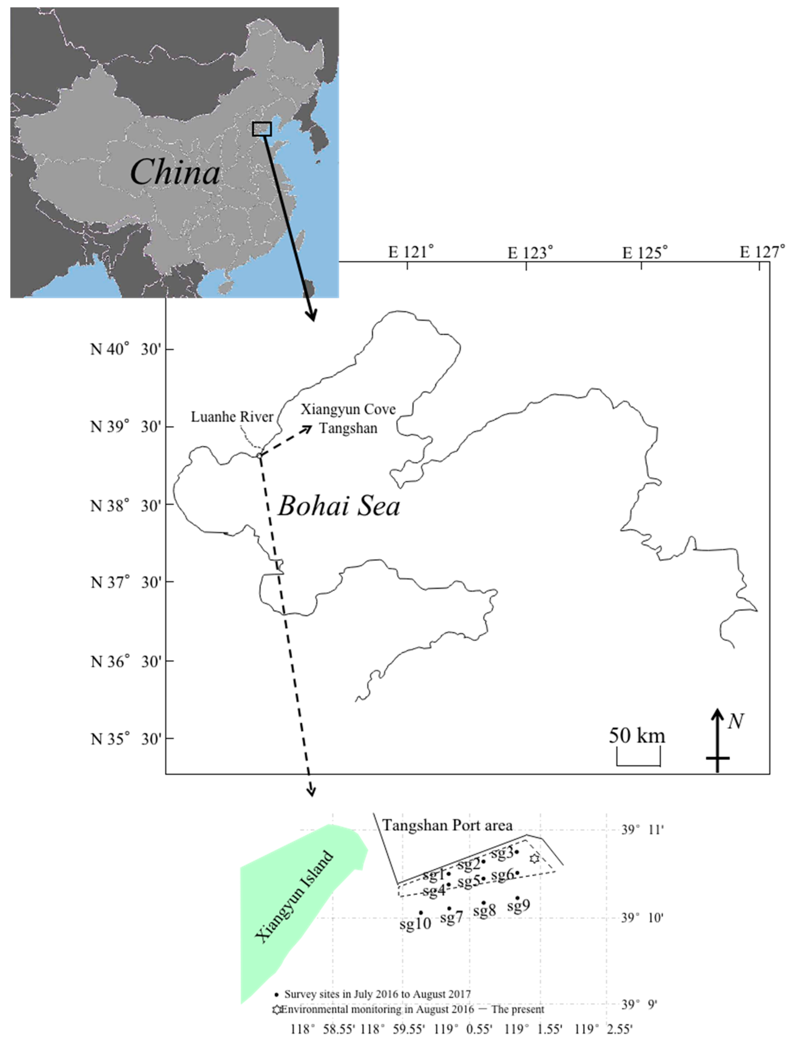
2.2. Study Area and Sampling

The Bohai Sea is a semi-closed shallow sea with a mean depth of 18 m. Our study area (39°10′14.78′′–39°10′53.86′′ N, 118$°$59′30.57′′–119$°$1′48.72′′ E) is located at 39°08′ N of Xiangyun Cove adjacent to Xiangyun Island and Tangshan Port (see Figure 1). The study area consists of a large number of artificial oyster–macroalgal reefs that were created within a ~2 km² area in July 2016. We collected phytoplankton samples at stations sg1–sg6 (in the reef area) and sg7–sg10 (in the control area) in July 2016 (before reef construction) and after reef construction (September 2016; May, June, and August 2017) via water sampling (Figure 1). We established a fixed environmental monitoring station to continually measure the environmental factors including water temperature, salinity, turbidity, DO, chlorophyll a, and total dissolved solids content via multiple sensors of a YSI EXO2 multi-parameter integrated water quality instrument (Sondes, Shanghai, China) at an interval of 10 min in the reef area during the survey period (Figure 1). We identified the flood and dry season of Luanhe River runoff according to the temporal variations in sea surface salinity measured at the fixed station.

We collected surface and bottom seawater at each station using a 5 L organic glass water container, and then mixed the collected samples in a 10 L organic glass water container. After full and uniform mixing, we collected 500 mL samples in a 500 mL organic glass water container and added Lugol’s reagent to fix the samples. This process was repeated for three replicates. After maintaining the samples with no movement for 48 h, we extracted the supernatant using a siphon tube and concentrated each sample into 25 mL volumes for storage. We placed a 0.1 mL sample in a 0.1 mL counting box (20 mm × 20 mm) and used a 40 × 10 times optical microscope mirror (Olympus, CX41-12C02, Tokyo Japan) to identify the species [23,24,25] and count the number of individuals of each species present. We counted twice for each sample and took the average value. If the difference was >15% between each counting result and the average value of the two counts, we counted the third one for the sample and took the average value.

2.3. Data Analysis

The abundance was calculated using the following formula [26]:

C = (n × V₁)/(V₂ × V_n)

where C is the average abundance (cells L^–1) of reef and control area during each survey; n is the count number of individuals in a 1 mL water sample after concentration (cell); V₁ is the volume after concentration (mL); V₂ is the real volume in 5 L of collected water samples; and V_n is the volume of the count box in 0.1 mL based on the observation made using the counting box.

The degree of dominance of a species during the survey was calculated using the following formula [27]:

$$Y={(n}_{\mathrm{i}}/N){\times f}_{\mathrm{i}}$$

where Y is the degree of dominance of a species at a station; n_i is the number of individuals of a species (inds); N is the total number of individuals of all species (inds); and f_i denotes the occurrence frequency of the ith species. Species with Y ≥ 0.02 were considered to be dominant species.

The Shannon–Weaver diversity index (H′), Pielou’s evenness index (J), and Margalef’s richness index (D) were used to analyze the community structure and diversity of phytoplankton. The indexes were calculated using the following formulas [28,29,30]:

$$H^{\prime }=-{\sum }_{n_i}^S{P}_i{\log }_2{P}_i$$

$$J=H^{\prime }/{\log }_{2}S$$

$$D=\left(S-1\right)/{\mathrm{l}\mathrm{o}\mathrm{g}}_{2}N$$

where P_i is the proportion of total samples’ number (N) belonging to ith species; S is the total species number in a station; N is the total species number; and n_i is the ratio of the species ith’s number to the total sample number.

The niche is important to revealing biota structure and species diversity [31], and the niche width index can measure the ability of a species to adapt to environments and resources [32]. The niche width index was calculated as follows [33]:

$$B_i={\displaystyle \frac{1}{r}}\times \sum _{j=1}^r{P}_{ij}^2$$

where B_i is the niche width of the ith species; P_ij is the ratio of the ith species abundance at station j to the total abundance at station j; and r is the total station number.

The niche overlap index is similar to niche width, and it reflects the degree of common utilization of the same natural resources by different groups. The niche overlap index was calculated using the following formula [34]:

$$O_{ik}={\displaystyle \frac{{\sum }_{j=1}^r(P_{ij}\times P_{kj})}{\sqrt{{\sum }_{j=1}^N{P}_{ij}^2}\times {\sum }_{j=1}^N{P}_{kj}^2}}$$

where $O_{ik}$ is the niche overlap index value, which ranges from 0 to 1. When $O_{ik}$ is >0.3, the niche overlap of species pairs is positive; at $O_{ik}$ > 0.6, the niche overlap of species pairs is significant. P_ij and P_kj represent the proportion of species i and species k in the jth sampling stations among all individuals of the species, respectively. r is the total number of sampling stations.

The overall association among species shows the stage of community succession and stability. Positive associations between species pairs means that the interactions are mutually beneficial [33]. Interspecific association (or variance ratio, V) was calculated as follows [35]:

$$\sum {\delta }_i^2=\sum _{i=1}^S{P}_i{\left(1-P_i\right)}^2$$

$$S_T^2=1/N\times {\sum }_{j=1}^N{\left(T_j-t\right)}^2$$

$$V={\displaystyle \frac{S_T^2}{{\delta }_i^2}}$$

where $\sum {\delta }_i^2$ represents the variance of the species occurring in all sampling stations; P_i represents the ratio of the number of sampling stations in which species i occurs to the total number of sampling stations; S represents the total species number; S_T² represents the variance of the occurrence frequency of the total species number; and T_j represents the number of dominant species that occur in sampling station j. t represents the average number of dominant species present in the sampling stations, with t = (T₁ + T₂ + … + T_n)/N. When V is <1, the overall correlation between the species is negative; at V > 1, the overall relationship between the species is positive; V = 1 is consistent with the assumption that all species are unrelated [36].

An interspecific association analysis can help clarify the succession and development dynamics of communities. We conducted the x² test using Yates’ continuous correction to compare the temporal differences in a study area [37]:

$$x^2={\displaystyle \frac{{n\times \left[\left|a\times d-b\times c\right|-0.5\times n\right]}^2}{\left(a+b\right)\times \left(a+c\right)\times \left(b+d\right)\times \left(c+d\right)}}$$

where n is the total number of sampling stations in the study area during one cruise; a is the number of sampling stations in which a pair of species occur together; b and c are the occurring numbers of sampling stations in the study area of a pair of species, respectively; and d is the number of sampling stations where a pair of species do not co-occur. Because x²_0.01 = 6.635 and x²_0.05 = 3.841, when x² > 3.841, the interspecific association of species pairs was significant; when x² > 6.635, it was extremely significant; and when x² < 3.841, it was not significant.

The co-occurrence percentage value indicates the degree of the connection of the non-significant species pairs assessed by the x² test, and the result can enhance the degree of significance of the species pairs that occur together. Therefore, we calculated the co-occurrence percentage value to verify the presence or absence of a non-significant intermediate connection in the x² test to ensure the accuracy of the results. The co-occurrence percentage (PC) calculation was calculated as follows [38]:

$$PC={\displaystyle \frac{a}{a+b+c}}$$

where the range of PC values is 0 ≤ PC ≤ 1. A higher PC value indicates a stronger interspecific association, and a lower value indicates a weaker association. PC = 0 indicates no interspecific association.

Finally, we used one-way ANOVA to determine the statistical differences in abundance among months via the software DPS platform [39].

3. Results

3.1. Species Composition, Dominant Species, and Abundance

We found three phytoplankton phyla (diatoms, dinoflagellates, silicoflagellates) consisting of 79 species in our study area, with 58 species of diatoms, 20 dinoflagellate species, and 1 silicoflagellate species (Figure 2a). The number of diatom species increased monthly in the following order: September 2016 > August 2017 > July 2016 > June 2017 > May 2017. For dinoflagellates, the number of species changed as follows: July 2016 > September 2016 > May 2017 > August 2017 > June 2017 (Figure 2a).

When we compared the species composition in July 2016 with that in June 2017, we found that the species for which abundance was lower before vs. after reef construction included Amphora lineolata, Coscinodiscus radiatus, Guinardia delicatula, Nitzschia longissma, Nitzschia lorenziana, P. sulcata, Pleurosigma angulatum, and Thalassionema nitzschioides. Species that were more abundant before than after reef construction included Pseudo-nitzschia pungens and N. scientillans (

Table 1. The species composition of phytoplankton (diatoms, dinoflagellates, silicoflagellates) in July and September 2016 and May, June, and August 2017. The total number of individuals (inds) is denoted by an Arabic integer, niche width is indicated within square brackets ‘[]’, and degree of dominance is shown within parentheses ‘()’. Before and After mean before and after the reef construction. The species marked in red are red tide species.

Species Name	Before	After
		Flood	Dry	Dry	Flood
	July 2016	September 2016	May 2017	June 2017	August 2017
Diatoms
1. Actinoptychus sp.	135	45	45
2. Amphora lineolata	180	225	90	3105 [0.0837] (0.03)	1850
3. Asterionella glacialis					200
4. Bacillaria paxillifera	450
5. Bacteriastrum sp.					100
6. Bellerochea malleus	90
7. Chaetoceros decipiens		5220
8. Chaetoceros atlanticus		1620
9. Chaetoceros curvisetus		80,658 [0.0364] (0.21)			136,000 0.0131 (0.38)
10. Chaetoceros debilis		270
11. Chaetoceros densus		2385			1500
12. Chaetoceros eibenii	225	1170
13. Chaetoceros lorenzianus		6255			9150 [0.0121] (0.03)
14. Chaetoceros peruvianus	270	540
15. Chaetoceros sp.	135	62,865 [0.0259] (0.14)			400
16. Climacodium frauenfeldianum				90
17. Corethron hystrix		45
18. Coscinodiscus gigas		45
19. Coscinodiscus granii					150
20. Coscinodiscus radiatus	135	135	4275 [0.0205] (0.11)	270	75
21. Coscinodiscus sp.	810	2790	6615 [0.0148] (0.19)	5310 [0.0186] (0.04)	9600 [0.0109] (0.03)
22. Cyclotella sp.	360	45		360	1200
23. Detonula pumila	315	35,118 [0.0908] (0.08)
24. Ditylum brightwellii		90	90		1700
25. Entomoneis alata	585
26. Eucampia zodiacus		81,675 [0.0713] (0.14)			31,100 [0.0281] (0.07)
27. Guinardia delicatula	90	1080		450
28. Guinardia striata	315	585			1700
29. Helicotheca tamesis	180				50
30. Hemiaulus sinensis		90
31. Leptocylindrus danicus	180	6570			5100
33. Meuniera membranacea	45
34. Navicula sp.	675	135	472.5	630	50
35. Nitzschia closterium					1550
36. Nitzschia longissma	1395	540		3285 [0.0593] (0.02)	50
37. Nitzschia lorenziana	315			2970 [0.0203] (0.02)	100
38. Nitzschia sp.	360	2880	45	5085 [0.059] (0.03)	2850
39. Odontella sinensis		450			13,650 [0.0123] (0.04)
40. Paralia sulcata	4995 [0.0396] (0.08)	315	21,105 [0.0156] (0.62)	5895 [0.0443] (0.04)	950
41. Pinnularia sp.	630	180	225	45
42. Planktoniella blanda	45
43. Pleurosigma angulatum	1170 [0.023] (0.02)	2250	540	2385
44. Pleurosigma pelagicum					100
45. Pleurosigma sp.					1800
46. Proboscia alata	45	990			75
47. Pseudo-nitzschia delicatissima	17,415 [0.3084] (0.11)	225
48. Pseudo-nitzschia pungens	11,790 [0.104] (0.18)	14,130 [0.0167] (0.04)		630
49. Rhizosolenia setigera		517.5	45		1225
50. Skeletonema costatum					76,150 [0.0113] (0.21)
51. Skeletonema sp.		180 [0.0397] (0.03)	135	66,375 [0.0141] (0.68)
52. Stephanopyxis palmeriana		1620			21,250 [0.014] (0.06)
53. Surirella sp.	270	45
54. Thalassionema frauenfeldii	45	855
55. Thalassionema nitzschioides	90	585		1035
56. Thalassiosira rotula		1755			29,350 [0.0113] (0.08)
57. Thalassiosira sp.		180	135	135	3500
58. Thalassiothrix franuenfeldii					50
Dinoflagellates
59. Akashiwo sanguinea		90
60. Alexandrium catenella	270	4140
61. Ceratium furca		180 [0.0315] (0.02)
62. Ceratium fusus	45
63. Ceratium macroceras	45		45
64. Ceratium tripos		540	135
65. Dinophysis caudata		90
66. Gymnodinium sp.	90
67. Gyrodinium spirale		585
68. Noctiluca scientillans	360	585		135	800
69. Ornithocercus steinii		45
70. Prorocentrum dentatum	135
71. Prorocentrum minimum	90
72. Prorocentrum sp.	990
73. Protoperidinium divergens	45
74. Protoperidinium ovum	90	45
75. Protoperidinium pallidum	45		45
76. Protoperidinium sp.	90	630			350
77. Pyrophacus steinii	45		90
78. Scrippsiella trochoidea	270
Silicoflagellates
79. Dictyocha fibula	45	1215			1050

).

We found more species of diatom in the reef area than in the control area in September 2016, May 2017, and August 2017; the exception was June 2017. A similar number of dinoflagellate species were present in the reef and control areas in each survey month after reef construction (Figure 2b).

The species only occurring in July 2016 were Bacillaria paxillifera, Bellerochea malleus, Entomoneis alata, Meuniera membranacea, Planktoniella blanda, C. fusus, Prorocentrum dentatum, Prorocentrum minimum, Protoperidinium divergens, and Scrippsiella trochoidea. The species that were present only after reef construction were Asterionellqa glacialis, Chaetoceros decipiens, Chaetoceros atlanticus, Chaetoceros debilis, Chaetocerus densus, Climacodium frauenfeldianum, Corethron hystrix, Coscinodiscus gigas, Coscinodiscus granii, Hemiaulus sinensis, Nitzxchia closterium, Pleurosigma pelagicum, Thalassionema franuenfeldii, Akashiwo sanguinea, Ceratium tripos, Dinophysis caudata, Gyrodinium spirale, and Ornithocercus steinii (Table 1).

The dominant species that occurred only after reef construction were Chaetoceros curvisetus, Chaetoceros lorenzianus, Eucampia zodiacus, Odentella sinensis, Skeletonema costatum, Stephanopyxis palmeriana, Thalassiosira rotula, Ceratium furca, Ditylum brightwellii, and Rhizosolenia setigera. The dominant species before and after reef construction included P. sulcata, P. pungens, and P. angulatum. The species for which abundance did not change after reef construction included Guinardia striata, Helicotheca tamesis, Ceratium macroceras, Pyrophacus steinii, Protoperidinium ovum, N. scientillans, and Proboscia alata. The species becoming dominant species and occurring both before and after the construction included A. lineolata, C. radiatus, Detonula pumila, Leptocylindrus danicus, N. longissma, N. lorenziana, T. nitzschioides, Alex andrium catenella, and Dictyocha fibula. These results show that some dominant species before reef construction became non-dominant species after construction, including Pseudo-nitschia delicatissima and Pinnularia sp. (Table 1).

The sums of each abundance in the study stations (reef plus control area) of each survey month ranged from 34,132.5 to 360,075 cells L^–1. The monthly average was 177,799.2 cells L^–1 before reef construction and 210,650.25 cells L^–1 after construction, and the abundances were as follows: August 2017 (flood season) > September 2016 (flood season) > June 2017 (dry season) > July 2016 > May 2017 (dry season) (Figure 3a). Minimum values for each month were in the following order: August 2017 > September 2016 > June 2017 > May 2017 > July 2016; maximum values were as follows: September 2016 > August 2017 > July 2016 > June 2017 > May 2017 (Figure 3b).

We found that the abundance of phytoplankton in July 2016 (before construction) differed significantly from that in September 2016 (p < 0.05), and it was extremely different from that in August 2017 (after construction) (p < 0.01). Additionally, the phytoplankton abundance in September 2016 (flood season) was extremely significantly different from that in May 2017 (dry season) (p < 0.01) and significantly different from that in June 2017 (dry season) (p < 0.05).

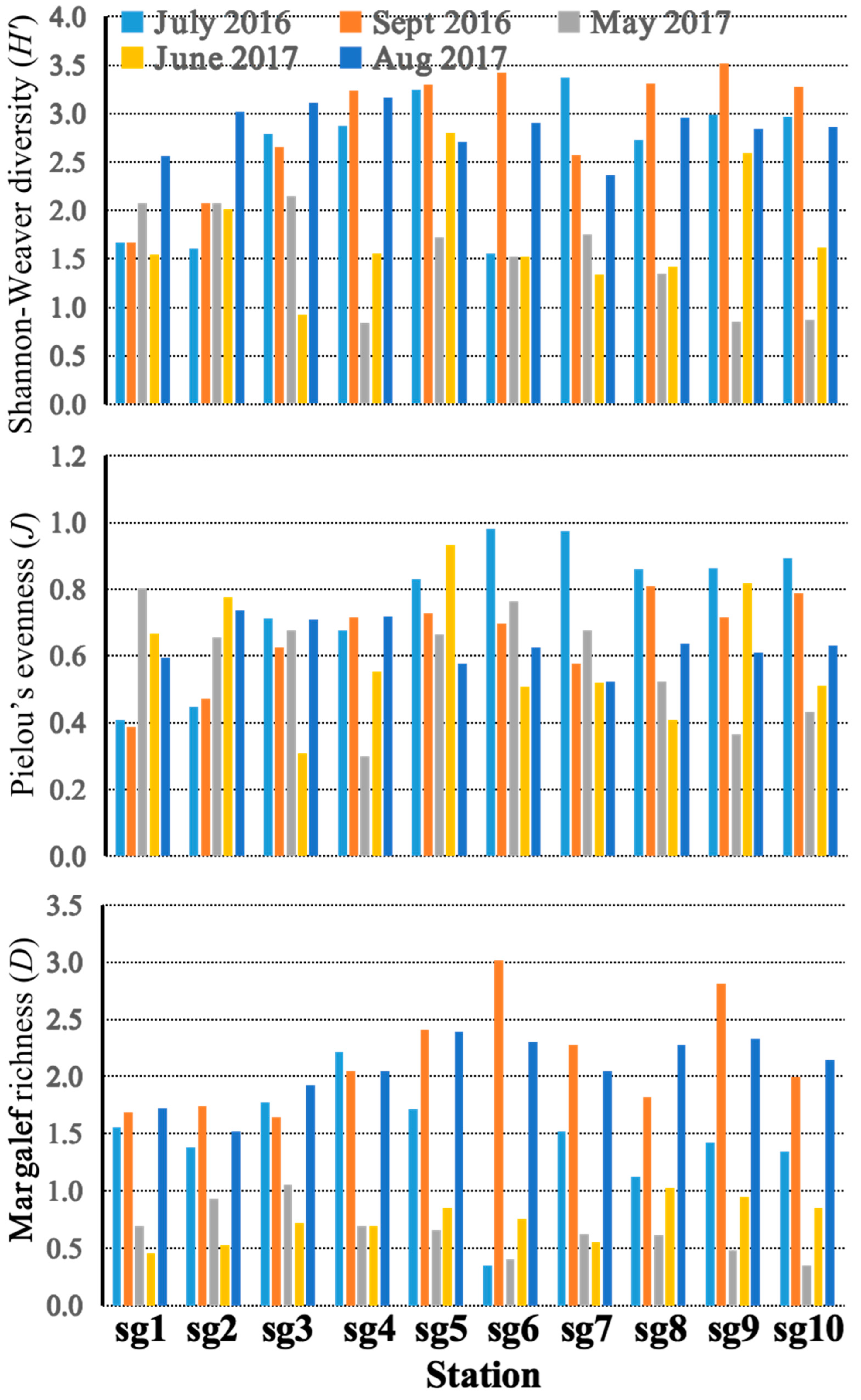
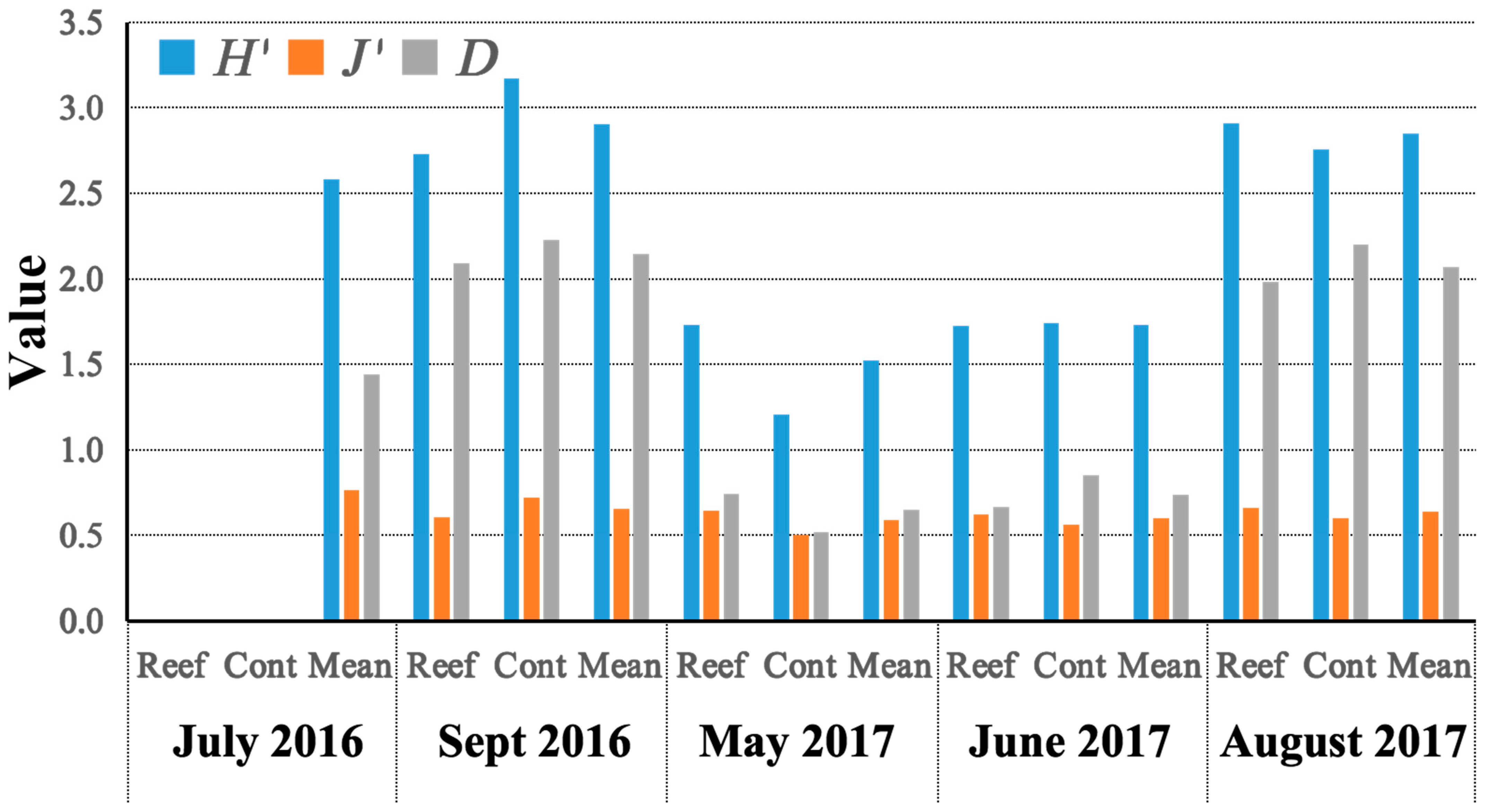
3.2. Diversity, Niche Width, Niche Overlap, and Interspecific Connection

The values of the diversity index (H′) in the reef area were in the following temporal order: August 2017 > September 2016 > July 2016 > the average value of the survey months > May and June 2017. Evenness index (J’) values in the reef area were in the temporal order of July 2016 > August 2017 > the average value of the survey months and May 2017 > June 2017 > September 2016. These values indicate a stable community structure before reef construction and increasing stability over time after the construction. In terms of species richness (D) in the reef area, the values were in the following temporal order: September 2016 > August 2017 > July 2016 > the average value of the survey months > May 2017 > June 2017 (Figure 4 and Figure 5).

The niche width of dominant species in July 2016 ranged from 0.023 to 0.3084, and greater niche width values after reef construction were detected for D. pumila (September 2016), A. lineolata (June 2017), E. zodiacus (September 2016 and August 2017), and N. longissima (June 2017) (Table 1). Regarding niche overlap, species with greater index values utilize more resources. In July 2016, the niche overlap index value of P. delicatissima and P. pungens was 0.9937, whereas that of P. sulcata and P. angulatum was 0.4118. Pairwise comparisons with O_ik > 0.6 in September 2016 were C. curvisetus and Chaetoceros sp., C. curvisetus and D. pumila, Chaetoceros sp. and E. zodiacus, Chaetoceros sp. against P. pungens, Chaetoceros sp. and Skeletonema sp., E. zodiacus and Skeletonema sp., P. pungens and Skeletonema sp., and P. pungens and C. furca. Pairs with O_ik > 0.6 in May 2017 were Coscinodiscus sp. and C. radiatus and Coscinodiscus sp. and P. sulcata. Pairwise comparisons with O_ik > 0.6 in June 2017 were A. lineolata and Skeletonema sp., Coscinodiscus sp. and Nitzschia sp., Coscinodiscus sp. and N. lorenziana, Coscinodiscus sp. and Skeletonema sp., Nitzschia sp. and N. longissima, Nitzschia sp. and P. sulcata, N. longissima and P. sulcata, and N. lorenziana and Skeletonema sp. With the exception of the pair Coscinodiscus sp. and E. zodiacus, all other pairs had O_ik values > 0.6 in August 2017 (

Table 2. Values of the niche overlap index among different dominant phytoplankton species pairs in July and September 2016 and May, June, and August 2017.

July 2016
	P. sulcata	P. angulatum	P. delicatissima	P. pungens
P. sulcata	1.0000
P. angulatum	0.4118	1.0000
P. delicatissima	0.0046	0.1725	1.0000
P. pungens	0.0300	0.1917	0.9937	1.0000
September 2016
	C. curvisetus	Chaetoceros sp.	D. pumila	E. zodiacus	P. pungens	Skeletonema sp.	C. furca
C. curvisetus	1.0000
Chaetoceros sp.	0.6453	1.0000
D. pumila	0.9486	0.5241	1.0000
E. zodiacus	0.1875	0.8005	0.1046	1.0000
P. pungens	0.5720	0.7483	0.3907	0.3528	1.0000
Skeletonema sp.	0.1991	0.7781	0.0290	0.7634	0.6630	1.0000
C. furca	0.1415	0.3408	0.0630	0.0885	0.6235	0.2497	1.0000
May 2017
	Coscinodiscus sp.	C. radiatus	P. sulcata
Coscinodiscus sp.	1.0000
C. radiates	0.7474	1.0000
P. sulcate	0.6684	0.4107	1.0000
June 2017
	A. lineolata	Coscinodiscus sp.	Nitzschia sp.	N. longissima	N. lorenziana	P. sulcata	Skeletonema sp.
A. lineolata	1.0000
Coscinodiscus sp.	0.5447	1.0000
Nitzschia sp.	0.5878	0.7189	1.0000
N. longissima	0.2181	0.5899	0.8512	1.0000
N. lorenziana	0.3821	0.7208	0.2063	0.2564	1.0000
P. sulcata	0.5321	0.5144	0.8186	0.7398	0.1646	1.0000
Skeletonema sp.	0.6577	0.6695	0.5849	0.5282	0.6355	0.3895	1.0000
August 2017
	Coscinodiscus sp.	C. curvisetus	C. lorenzianus	E. zodiacus	O. sinensis	S. costatum	S. palmeriana	C. furca
Coscinodiscus sp.	1.0000
C. curvisetus	0.8680	1.0000
C. lorenzianus	0.9349	0.8980	1.0000
E. zodiacus	0.5811	0.6069	0.6909	1.0000
O. sinensis	0.8532	0.6515	0.7596	0.6536	1.0000
S. costatum	0.8686	0.8388	0.8621	0.6809	0.9154	1.0000
S. palmeriana	0.8192	0.8057	0.8528	0.9082	0.8064	0.8217	1.0000
C. furca	0.9477	0.9397	0.9502	0.6964	0.8206	0.8999	0.8770	1.0000

).

The variance ratios (V) of the dominant species were 3.69 and 2.5–10 before and after reef construction, with an average of 5.17. The monthly variations in the values were in the following order: May 2017 > August 2017 > July 2016 > September 2016 > June 2017 (Figure 6). The comparison of A. lineolata and P. sulcata (1.28) and N. longissima and P. sulcata (2.1) had a greatest χ² value in June 2017. In addition, P. sulcata and P. angulatum as well as P. angulatum and P. pungens had a strong degree of connection (PC > 0.60) in July 2016. The pairs with PC > 0.60 in May 2017 were Coscinodiscus sp. and C. radiatus (or P. sulcata) as well as C. radiatus and P. sulcata (

Table 3. Results of χ² test and co-occurrence percentage values (in parentheses) showing degree of interspecific association among different dominant phytoplankton species in July and September 2016 and May, June, and August 2017.

July 2016
	P. sulcata	P. angulatum	P. delicatissima
P. angulatum	0.21 (0.78)
P. delicatissima	0.36 (0.25)	0.21 (0.33)
P. pungens	0.36 (0.56)	0.21 (0.78)	0.36 (0.25)
September 2016
	C. curvisetus	Chaetoceros sp.	D. pumila	E. zodiacus	P. pungens	Skeletonema sp.
Chaetoceros sp.	0.63 (0.70)
D. pumila	0.63 (0.89)	0.04 (0.78)
E. zodiacus	0.05 (0.67)	0.23 (0.56)	0.28 (0.56)
P. pungens	(0.90)	(0.89)	(0.89)	(0.75)
Skeletonema sp.	0.21 (0.60)	0.03 (0.50)	0.03 (0.50)	0.18 (0.44)	(0.70)
C. furca	0.63 (0.70)	0.04 (0.60)	0.04 (0.60)	0.23 (0.40)	(0.80)	0.02 (0.73)
May 2017
	Coscinodiscus sp.	C. radiatus
C. radiatus	(0.90)
P. sulcata	(1.00)	(0.90)
June 2017
	A. lineolata	Coscinodiscus sp.	Nitzschia sp.	N. longissima	N. lorenziana	P. sulcata
Coscinodiscus sp.	0.04 (0.60)
Nitzschia sp.	1.28 (0.75)	1.28 (0.75)
N. longissima	0.23 (0.40)	0.06 (0.56)	2.1 (0.33)
N. lorenziana	0.04 (0.60)	0.04 (0.60)	0.23 (0.40)	0.23 (0.56)
P. sulcata	1.28 (0.75)	0.23 (0.40)	0.02 (0.50)	2.1 (0.33)	4.4 (0.40)
Skeletonema sp.	(1.00)	(0.80)	(0.60)	(0.60)	(0.80)	(0.60)
August 2017
	Coscinodiscus sp.	C. curvisetus	C. lorenzianus	E. zodiacus	O. sinensis	S. costatum	S. palmeriana
C. curvisetus	(1.00)
C. lorenzianus	(1.00)	(1.00)
E. zodiacus	(0.80)	(0.90)	(0.80)
O. sinensis	(1.00)	(1.00)	(1.00)	(0.80)
S. costatum	(1.00)	(1.00)	(1.00)	(0.80)	(1.00)
S. palmeriana	(1.00)	(1.00)	(1.00)	(0.80)	(1.00)	(1.00)
T. rotula	(1.00)	(1.00)	(1.00)	(0.80)	(1.00)	(1.00)	(1.00)

).

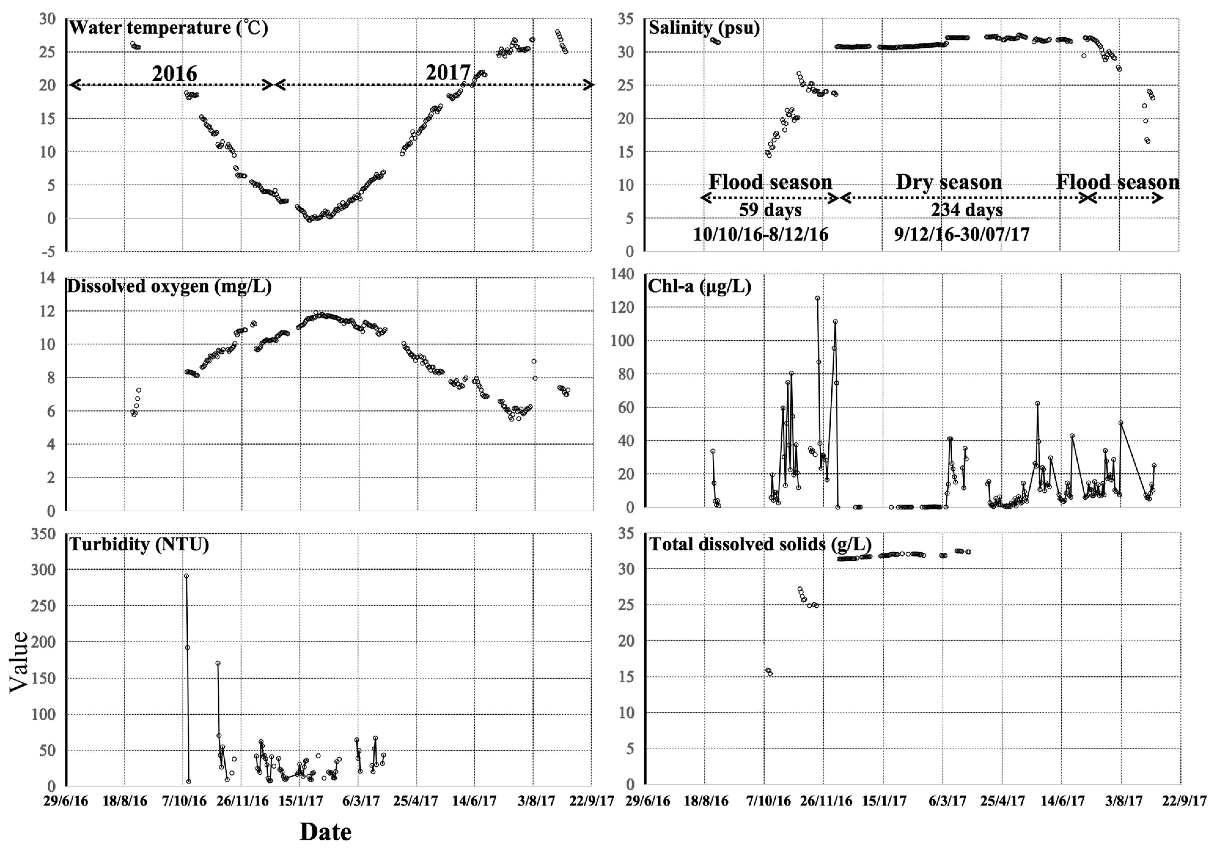
3.3. Temporal Variations in Environmental Factors

Environmental factors also varied over the course of the study (Figure 7). The surface water temperature decreased from 26.257 °C on 25 August 2016 to −0.32 °C on 24 January 2017, with a daily average decrease in water temperature of 0.175 °C/day. It then increased to the peak value of 28.024 °C on 24 August 2017, with a daily average increase in water temperature of 0.134 °C/day, and then decreased to 25.021 °C on 31 August 2017. The numbers of days of increasing and decreasing water temperature were 153 and 212, respectively. Water temperature was >20 °C from 25 August to 30 in 2016 and from 13 June to 31 August in 2017.

The average surface salinity in August 2016 was 31.596 psu, which was during the dry season of the Luanhe River. The salinity slowly increased from 14.92 psu on 10 October to 30.75 psu on 8 December 2016, which represents 59 days in which the average increase was 0.268 psu/day. This occurred during the flood season, but the Luanhe River runoff gradually decreased and exhibited time variations. The salinity range of the estuarine area of the Luanhe River was 28.79 to 32.52 psu from 9 December 2016 to 30 July 2017; during this dry season, a small fluctuation of salinity occurred. The salinity decreased from 27.688 psu on 2 August 2017 to 16.54 psu on 27 August 2017, with a daily average decrease in salinity of 0.45 psu/day (indicating the beginning of the flood season), and then it increased to 23.062 psu/day on 31 August 2017.

The turbidity of the water from 10 to 11 October to 6 to 7 November 2016 was > 100. The average values of turbidity from 9 December 2016 to 4 January 2017 and from 13 January to 28 March 2017 were 27.212 and 27.173 NTU, respectively. The number of days during the dry season (234 days) was far greater than that of flood seasons (59 days). DO content increased from 5.77 mg L^–1 on 26 August 2016 to 11.91 mg L^–1 on 28 January 2017 (155 days) and then decreased to 5.54 mg L^–1 on 20 July 2017 (157 days). Chl-a content fluctuated greatly during the flood season but very little during the dry season. Chl-a content > 10 μg L^–1 occurred on 25–26 August 2016; 5 October–5 November 2016; 23 October–5 November 2016; 15 November–7 December 2016; 11–26 March 2017; 23 May–5 June 2017; 19 June–3 August 2017; and 29–31 August 2017. The periods during which Chl-a content was > 1 μg L^–1 and < 10 μg L^–1 were 27–29 August 2016; 13–19 October 2016; 15–24 April 2017; 3–16 May 2017; 12–22 June 2017; 4 July–2 August 2017; and 24–28 August 2017. The average values of total dissolved solids were 23.021 and 31.82 g L^–1, respectively, during the flood season of 10 October to 20 November 2016 and the dry season of 9 December 2016 to 28 March 2017.

4. Discussion

In our study area, we identified 58 species of diatoms and 20 species of dinoflagellates. Li (2016) estimated the sinking rate of N. scintillans (N. scientillans in our study) to be 0.13 m/day, implying that it takes 154 days to sink from the sea surface to the bottom, assuming a depth of 20 m [40]. The small- to medium-sized diatom species such as N. closterium and S. costatum found in our study were also reported to be usually abundant in Tiahura Reef waters [41]. The diatom species Asterionella glacialis is a common near-shore and estuarine phytoplankton species [42] that is frequently present and abundant in coastal regions such as the study area. The dominant diatom species (Coscinodiscus sp. and P. sulcata) in our study are benthic species in temperate waters [43,44]. Chaetoceros spp. and P. sulata dominated in the Bohai Sea from spring to autumn [45]. The number of Coscinodiscus sp. individuals is gradually increasing in the Bohai Sea, and it is a red tide species in China [46,47]. In addition, the benthic/epibenthic species Pleurosigma sp. was present in a high abundance in our study. We also found several chain-forming species in the estuarine area, such as Chaetoceros spp., L. danicus, and G. delicatula.

Diversity indexes are often used to assess the complexity of community structure; when a community is more complex, and the feedback function to the environment is stronger, the community structure is buffered and tends to be stable. The values of the diversity (2.29), evenness (0.68), and richness (1.50) indexes in our study before reef construction were similar to those reported for the Nanri Island artificial reef area (2.206, 0.464, and 1.75, respectively) [48]. After reef construction, the values (2.28, 0.64, and 1.40) in our study were lower than those (3.424, 0.672, and 2.504) of Nanri Island [48]. In addition, no obvious difference between the artificial reef areas of Nanri Island [48], Li Island of Rongcheng [49], Xiangshan Bay [50], Daya Bay [51], and Haizhou Bay [52] were reported. These results suggest that phytoplankton were equally abundant throughout the area and that a balance between artificial reefs and the surrounding area developed. In our study, the values of the diversity and evenness indexes were higher in reef (against control) and control (against reef) areas, respectively, in May, June, and August 2017 and in July and September 2016. The values of the richness indexes were higher in reef and control areas, respectively, in July 2016 and May 2017, and in September 2016 and June and August 2017. Thus, our results show that the variation in community diversity depended on the season. Similarly, Einbinder et al. (2006) showed that phytoplankton biomass in an artificial reef area was significantly higher than it was before the reef was built [53]. In Baiyangdian Lake, the values of the diversity and evenness indexes increased month by month around the area of the artificial reef [54]. Xu et al. (2017) also reported higher values of the diversity index in the reef area compared with the control area in Qinhuangdao [55]. The abundance of phytoplankton in our study area increased from March to August (34,132.50 to 360,075.00 cells L^–1). Yu et al. (2024) reported an average phytoplankton abundance of 18.30–1428.10 × 10⁴ cells m^–3 with an annual average value of 18.30–313.50 × 10⁴ cells m^–3, in the reef area of Xiangyun wan [56]. They found that in summer, autumn, and winter, the H′, J′, and D values in the reef area were higher than those of the control area, and Coscinodiscus spp. and P. sulata dominated the communities in winter and spring, respectively [56]. Leon et al. (2011) argued that the abundance of phytoplankton undergoes significant seasonal variations, especially in temperate waters [57], and Lundberg et al. (2014) suggested that the greatest concentrations of Chl-a would occur during summer and autumn [58].

Many isotope and gut content studies have concluded that oysters consume phytoplankton and suspended benthic algae [59,60,61], although Fukumori et al. (2008) showed that cultured oysters consumed epiphytes growing on the reef [62]. Liang et al. (2020) found that scallop farming seldom suppressed the standing stock of phytoplankton, and they suggested that bottom-seeded scallops had no access to surface phytoplankton biomass [12]. Pomeroy et al. (2006) suggested that spatial mismatch between the peak time of filtration rates and abundance can prevent bivalves from bottom phytoplankton community control [63]. We found that oysters might suppress phytoplankton abundance in the summer. In addition, increases in phytoplankton are frequently followed by a bloom of benthic macroalgae, because macroalgal growth can prevent the loss of dissolved nutrients from the ecosystem. For example, Miller et al. (2011) found that after removing the canopies of the giant kelp Macrocystis pyrifera, production by phytoplankton was two times greater [1]. Following a natural decline in the Macrocystis canopy due to winter storms, production by phytoplankton eventually increased to levels that compensated for the loss of production by Macrocystis. In our study, the abundance of phytoplankton was lowest in the summer (May 2017), but macroalgae consumed a large amount of nutrients and were in a rapid growth stage, which created a competitive relationship between these primary producers.

Environmental conditions also might affect the structure of the phytoplankton community. Liu et al. (2024) assessed the main environmental variables impacting phytoplankton community structure with temporal–spatial variations in the sea areas of Huanghua Port in 2014, and found that water temperature and salinity were most important in spring; DO and salinity in summer; salinity, water temperature, and DO in autumn; and DO, water temperature, and PO₄-P in winter [64]. Seaman et al. (2000) suggested that stronger turbulence favors phytoplankton groups such as diatoms [65]. On the sea floor, artificial reefs are obstacles to currents, resulting in variability and intersecting flow fields that create an ideal environment for nutrient transport and promote a massive reproduction and growth of phytoplankton in the reef area. Silva et al. (2009) found that larger species such as Pseudo-nitzschia spp. and D. pumila occurred during the nutrient-rich upwelling conditions, and finally Dinophysis spp., Protoperidinium spp., and Ceratium spp. were detected [66].

Day et al. (2009) and Riekenberg et al. (2015) noted that the seasonal variations in the flow rate and nutrient concentrations within Breton Sound Estuary caused a shift in phytoplankton community assemblages [67,68]. Low discharge from the Luanhe River in the dry season leads to high salinity, decreased turbidity, low nutrient concentrations, and increased water body residence time. Salinity affects the distribution, abundance, and composition of phytoplankton groups. Although the high-water period was generally characterized by lower phytoplankton biomass in our study, we found higher phytoplankton abundance during the flood season of the Luanhe River. Similarly, Michael et al. (2005) reported large phytoplankton blooms in the Gulf of California (54–577 km²) fueled by nitrogen-rich agricultural runoff [69]. Temperature is another important factor that affects the growth and composition of the phytoplankton community. Laboratory studies suggested that for most phytoplankton species, optimum temperatures for growth are in the range of 20–25 °C [70]. Increased water temperature promotes metabolism and enzyme activity of phytoplankton, thereby promoting growth [71].

5. Conclusions

In summary, we report the following conclusions based on our data:

(1) Diatoms and dinoflagellates were the most representative groups in the phytoplankton community, with 79 species present in our samples.

(2) The total species number (not including diatoms) and abundance of phytoplankton increased from May to September, and the number of species present in the reef area was greater than the number outside of the reef area. The abundance in the western part of the survey area was higher than that of the eastern part. The abundance in August–September was higher in the reef area than in the control area, whereas the opposite was true in May–June.

(3) One year after reef construction, the species composition had changed, and A. lineolata, C. radiatus, G. delicatula, N. longissma, N. lorenziana, P. sulcata, P. angulatum, and T. nitzschioides became dominant as the abundance of P. pungens and N. scientillans decreased. Post-reef construction, P. sulcata and P. angulatum were the dominant species, and the abundances of G. striata, H. tamesis, C. macroceras, P. steinii, P. ovum, N. scientillans, and P. alata had not changed.

In the future, we will focus on quantifying the trophic linkages among phytoplankton, oysters, and benthic macroalgae that support fisheries’ production on temperate artificial reefs. We will also try to identify interactions among different producers and consumers in the oyster–macroalgae reef ecosystem and provide a more comprehensive understanding of how changes in the relative and absolute amounts of net primary production affect the community. It is crucial to continue to monitor primary productivity of macroalgae and phytoplankton, and an analysis of a series of annual data sets will increase our understanding of the temporal dynamics of the phytoplankton of this system. Our results provide important data that can be applied to the management and maintenance of artificial oyster–macroalgae reef ecosystems in sea ranch areas.

References

1. Miller, R.J.; Reed, D.C.; Brzezinski, M.A. Partitioning of primary production among giant kelp (Macrocystis pyrifera), understory macroalgae, and phytoplankton on a temperate reef. Limnol. Oceanogr. 2011, 56, 119–132. [Google Scholar] [CrossRef]
2. Daigle, S.T.; Fleeger, J.W.; Cowan, J.H., Jr.; Pascal, P.Y. What is the relative importance of phytoplankton and attached macroalgae and epiphytes to food webs on offshore oil platforms? Mar. Coast. Fish. 2013, 5, 53–64. [Google Scholar] [CrossRef]
3. Keerthi, M.G.; Prend, C.J.; Aumont, O.; Lévy, M. Annual variations in phytoplankton biomass driven by small-scale physical processes. Nat. Geosci. 2022, 15, 1027–1033. [Google Scholar] [CrossRef]
4. Ren, L.; Rabalais, N.N.; Turner, R.E. Effects of Mississippi river water on phytoplankton growth and composition in the upper Barataria Estuary, Louisiana. Hydrobiologia 2020, 847, 1831–1850. [Google Scholar] [CrossRef]
5. Bargu, S.; Justic, D.; White, J.R.; Lane, R.; Day, J.; Paerl, H.; Raynie, R. Mississippi River diversions and phytoplankton dynamics in deltaic Gulf of Mexico estuaries: A review. Estuar. Coast. Shelf Sci. 2019, 221, 39–52. [Google Scholar] [CrossRef]
6. Heil, C.A.; Revilla, M.; Glibert, P.M.; Murasko, S. Nutrient quality drives differential phytoplankton community composition on the southwest Florida shelf. Limnol. Oceanogr. 2007, 52, 1067–1078. [Google Scholar] [CrossRef]
7. Xu, M.; Yang, X.Y.; Song, X.J.; Xu, K.D.; Yang, L.L. Seasonal analysis of artificial oyster reef ecosystems: Implications for sustainable fisheries management. Aquac. Int. 2021, 29, 167–192. [Google Scholar] [CrossRef]
8. Xu, M.; Qi, Z.L.; Liu, Z.L.; Quan, W.M.; Zhao, Q.; Zhang, Y.L.; Liu, H.; Yang, L.L. Coastal aquaculture farms for the sea cucumber Apostichopus japonicus provide spawning and first year nursery grounds for wild black rockfish, Sebastes schlegelii: A case study from the Luanhe River estuary, Bohai Bay, the Bohai Sea, China. Front. Mar. Sci. 2022, 9, 911399. [Google Scholar] [CrossRef]
9. Xu, M.; Xu, Y.; Yang, J.; Li, J.X.; Zhang, H.P.; Xu, K.D.; Zhang, Y.L.; Otaki, T.; Zhao, Q.; Zhang, Y.; et al. Seasonal variations in the diversity and benthic community structure of subtidal artificial oyster reefs adjacent to the Luanhe River Estuary, Bohai Sea. Sci. Rep. 2023, 13, 17650. [Google Scholar] [CrossRef] [PubMed]
10. Santos, D.H.C.d.; Silva-Cunha, M.d.G.G.; Santiago, M.F.; Passavante, J.Z.d.O. Characterization of phytoplankton biodiversity in tropical shipwrecks off the coast of Pernambuco, Brazil. Acta Bot. Bras. 2010, 24, 924–934. [Google Scholar] [CrossRef]
11. Matisson, J.; Olof, L. Benthic macrofauna succession under mussels, Mytilus edulis L. (Bivalvia), cultured on hanging long-lines. Sarsia 1983, 68, 97–102. [Google Scholar] [CrossRef]
12. Liang, Y.; Zhao, Z.X.; Zhang, G.T.; Wang, S.W.; Wan, A.Y.; Liu, Q. Distinguishing nutrient-depleting effects of scallop farming from natural variabilities in an offshore sea ranch. Aquaculture 2020, 518, 734844. [Google Scholar] [CrossRef]
13. Wu, Y.G. Current status and future development suggestions of marine fisheries resources in Hebei Province. Hebei Fish. 1980, 3, 1–12. (In Chinese) [Google Scholar]
14. Xu, B.C.; Zhou, E.M.; Song, W.X. Distribution characteristics of surface temperature, salinity in the mouth of Luanhe River. Adv. Mar. Sci. 1986, 3, 126–133. (In Chinese) [Google Scholar]
15. Zhao, X.; Wei, Y.; Sun, J.; Zhang, G.; Zhao, L.; Jia, D. Picophytoplankton from Qinhuangdao coastal waters in spring and summer. Acta Oceanol. Sin. 2020, 42, 106–114. (In Chinese) [Google Scholar]
16. Luan, Q.; Kang, Y.; Wang, J. Long-term changes on phytoplankton community in the Bohai Sea (1959~2015). Prog. Fish. Sci. 2018, 39, 9–18. (In Chinese) [Google Scholar]
17. Fu, X.T.; Sun, J.; Wei, Y.Q.; Liu, Z.S.; Xin, Y.H.; Guo, Y.; Gu, T. Seasonal shift of a phytoplankton (>5 μm) community in Bohai Sea and the adjacent Yellow Sea. Diversity 2021, 13, 65. [Google Scholar] [CrossRef]
18. Luan, Q.; Kang, Y.; Wang, J. Long-term changes of phytoplankton community and diversity in adjoining waters of the Yellow River estuary (1960–2010). J. Fish. Sci. China 2017, 24, 913–921. (In Chinese) [Google Scholar] [CrossRef]
19. Chen, C.C.; Gong, G.C.; Shiah, F.K. Hypoxia in the East China Sea: One of the largest coastal low-oxygen areas in the world. Mar. Environ. Res. 2007, 64, 399–408. [Google Scholar] [CrossRef] [PubMed]
20. Wei, H.; Zhao, L.; Zhang, H.Y.; Lu, Y.Y.; Yang, W.; Song, G.S. Summer hypoxia in Bohai Sea caused by changes in phytoplankton community. Anthr. Coasts 2021, 4, 77–86. [Google Scholar] [CrossRef]
21. Ran, X.; Zang, J.; Wei, Q.; Guo, J.; Yi, X.; Liu, W.; Liu, J. Hypoxia and its cause of formation in the adjacent waters of Rushan Bay. Adv. Mar. Sci. 2012, 30, 347–356. (In Chinese) [Google Scholar]
22. Yang, D.; Zhou, Z.Q.; Zhang, J.S.; Liu, T.T.; Li, X.J.; Ai, B.H.; Li, B.Q.; Chen, L.L. Characteristics of macrobenthic communities at the Muping marine ranch of Yantai in summer. Mar. Sci. 2017, 41, 134–143. (In Chinese) [Google Scholar]
23. Yang, S.M.; Dong, S.G. Zhongguohaiyuchangjianfuyouguizaotupu (Atlas of Common Plankton Diatoms in China Seas); China Ocean University Press: Qingdao, China, 2006. (In Chinese) [Google Scholar]
24. Qian, S.B.; Liu, D.Y.; Sun, J. Marine Phycology; China Ocean University Press: Qingdao, China, 2014. (In Chinese) [Google Scholar]
25. Guo, Y.J.; Qian, S.B. Bacillariophyta; Science Press: Beijing, China, 2017. (In Chinese) [Google Scholar]
26. State Oceanic Administration. Specifications of Oceanographic Survey: GB12763.6-2007[S]; China Standard Press: Beijing, China, 2008; pp. 34–38. (In Chinese) [Google Scholar]
27. McNaughton, S.J. Relationships among functional properties of Californian grassland. Nature 1967, 216, 168–169. [Google Scholar] [CrossRef]
28. Shannon, C.E.; Weaver, W. The Mathematical Theory of Communications; University of Illinois Press: Urbana, IL, USA, 1949. [Google Scholar]
29. Pielou, E.C. The measurement of diversity in different types of biological collections. J. Theor. Biol. 1966, 13, 131–144. [Google Scholar] [CrossRef]
30. Margalef, R. Information theory in ecology. Gen. Syst. 1958, 3, 36–71. [Google Scholar]
31. Hurlbert, S.H. The measurement of niche overlap and some relatives. Ecology 1978, 59, 67–77. [Google Scholar] [CrossRef]
32. Chen, D.Q. Guidelines for Investigation of River Hydrobiology; Science Press: Beijing, China, 2014; pp. 172–286. ISBN 978-7-03-039429-3. (In Chinese) [Google Scholar]
33. Levins, R. Evolution in Changing Environments: Some Theoretical Explorations; Princeton University Press: Priceton, NJ, USA, 1968. [Google Scholar]
34. Pianka, E.R. The structure of lizard communities. Annu. Rev. Ecol. Syst. 1973, 4, 53–74. [Google Scholar] [CrossRef]
35. Charles, K. Ecological Methodology; Harper Collins Publishers: Now York, NY, USA, 1989; ISBN 0321021738. [Google Scholar]
36. Schluter, D. A variance test for detecting species associations, with some example applications. Ecology 1984, 65, 998–1005. [Google Scholar] [CrossRef]
37. Zhang, J.T. Quantitative Ecology; Science Press: Beijing, China, 2004; ISBN 9787030309372. (In Chinese) [Google Scholar]
38. Li, Z.L.; Zhang, H.Y.; Zhao, L.; Xu, F. Spatial and temporal distribution and factors influencing the phytoplankton community structure in the Bohai Sea. Mar. Sci. 2021, 8, 10–20. (In Chinese) [Google Scholar]
39. Tang, Q.Y.; Zhang, C.X. Data Processing System (DPS) sofware with experimental design, statistical analysis and data mining developed for use in entomological research. Insect Sci. 2013, 20, 254–260. [Google Scholar] [CrossRef]
40. Li, X.Q. The Study of Phytoplankton Sinking Rate in the Yellow Sea and Bohai Sea. Master’s Thesis, Tianjin University of Science & Technology, Tianjin, China, 2016; pp. 1–61. (In Chinese). [Google Scholar]
41. Delesalle, B.; Pichon, M.; Frankignoulle, M.; Gattuso, J. Effects of a cyclone on coral reef phytoplankton biomass, primary production and composition (Moorea island, French polynesia). J. Plankton Res. 1993, 15, 1413–1423. [Google Scholar] [CrossRef]
42. Johnson, W.S.; Allen, D.M. Zooplankton of the Atlantic and Gulf Coasts: A Guide to Their Identification and Ecology; The Johns Hopkins University Press: Baltimore, MD, USA, 2013; pp. 1–452. [Google Scholar]
43. Chen, N.S.; Huang, H.L. Advances in the study of biodiversity of phytoplankton and red tide species in China (1):Bohai Sea. Oceanol. Limnol. Sin. 2021, 52, 346–395. (In Chinese) [Google Scholar]
44. Chen, Y.; Wang, L.; Shang, H.X.; Ma, L.; Zhang, S.S.; Xu, Y. Community Structure and Correlations of Phytoplankton with Environmental factors in Coastal Aquaculture area in Dalian, Liaoning Province, China. Chin. J. Fish. 2023, 36, 60–66. (In Chinese) [Google Scholar]
45. Li, Y.; Zhang, Q.; Yang, S. Phytoplankton community structure and its seasonal variation in the Bohai Sea in 2021. Adv. Mar. Sci. 2024, 42, 337–348. (In Chinese) [Google Scholar]
46. Zhang, Q.F.; Yi, C.L.; Xu, Y.S.; Shi, H.M. The Phytoplankton Community Sampled by Nets in the Dominant Area Monitoring Red Tide in Bohai Bay in Summer, 2006. J. Tianjing Univ. Sci. Technol. 2007, 3, 19–23. (In Chinese) [Google Scholar]
47. Zhang, X.; Wang, J.; Ma, W.; Wang, H.; Gao, Y.; Liu, K.F. The net-phytoplankton community structure in the Bohai Sea in autumn 2014. Haiyangxuebao 2020, 42, 89–100. (In Chinese) [Google Scholar]
48. Yang, F. Community characteristics of phytoplankton in artificial reef area around Nanri islands in spring. J. Fish. Res. 2016, 38, 210–218. (In Chinese) [Google Scholar]
49. Liu, C.D.; Yi, J.; Guo, X.F.; Tang, Y.L.; Huang, L.Y. Phytoplankton community structure in artificial reef area around Lidao, Rongcheng, and its relationship with environmental factors. J. Ocean. Univ. China 2016, 46, 50–59. (In Chinese) [Google Scholar]
50. Jiang, Z.B.; Chen, Q.Z.; Shou, L.; Ling, Y.B.; Zhu, X.Y.; Gao, Y.; Zeng, J.N.; Zhang, Y.X. Community composition of net-phytoplankton and its relationship with the environmental factors at artificial reef area in Xiangshan Bay. Acta Ecol. Sin. 2012, 32, 5813–5824. (In Chinese) [Google Scholar] [CrossRef]
51. Liao, X.L.; Chen, P.M.; Ma, S.W.; Chen, H.G. Community structure of phytoplankton and its relationship with environmental factors before and after construction of artificial reefs in Yangmeikeng, Daya Bay. S. China Fish. Sci. 2013, 9, 109–119. (In Chinese) [Google Scholar]
52. Zhang, S.; Zhu, K.W.; Sun, M.C. Species composition and biomass variation in phytoplankton in artificial reef area in Haizhou Bay. J. Dalian Ocean. Univ. 2006, 21, 134–140. (In Chinese) [Google Scholar]
53. Einbinder, S.; Perelberg, A.; Ben-Shaprut, O.; Foucart, M.; Shashar, N. Effects of artificial reefs on fish grazing in their vicinity: Evidence from algae presentation experiments. Mar. Environ. Res. 2006, 61, 110–119. [Google Scholar] [CrossRef] [PubMed]
54. Zhu, H.; Liu, X.; Cheng, S.; Wang, J. Effects of Artificial Reefs on Phytoplankton Community Structure in Baiyangdian Lake, China. Water 2021, 13, 1802. [Google Scholar] [CrossRef]
55. Xu, Y.F.; Li, Y.Q.; Zhang, H.P.; Gao, W.B.; Wang, S.Z.; Hu, B.C.; Liu, S.J. Evaluation index system and case applications of ecological restoration effect in artificial fish (Macroalgae) reef areas. Hebei Fish. 2017, 1, 42–50. (In Chinese) [Google Scholar]
56. Yu, S.; Zhao, Q.; Li, J.D.; Zhao, J.B.; You, K.; Zhang, P. Temporal and spatial variation characteristics of net-collected phytoplankton Community Structure and its relationship with key environmental factors in the artificial reef area of Xiangyun Bay, Hebei Province. Haiyang Xuebao 2024, 46, 52–63. (In Chinese) [Google Scholar]
57. Leon, L.F.; Smith, R.E.; Hipsey, M.R.; Bocaniov, S.A.; Higgins, S.N.; Hecky, R.E.; Antenucci, J.P.; Imberger, J.A.; Guildford, S.J. Application of a 3D hydrodynamic–biological model for seasonal and spatial dynamics of water quality and phytoplankton in Lake Erie. J. Great Lakes Res. 2011, 37, 41–53. [Google Scholar] [CrossRef]
58. Lundberg, C.J.; Lane, R.R.; Day, J.W. Spatial and temporal variations in nutrients and water-quality parameters in the Mississippi River-influenced Breton Sound estuary. J. Coast. Res. Int. Forum 2014, 30, 328–336. [Google Scholar] [CrossRef]
59. Page, H.M.; Lastra, M. Diet of intertidal bivalves in the Rıa de Arosa (NW Spain): Evidence from stable C and N isotope analysis. Mar. Biol. 2003, 143, 519–532. [Google Scholar] [CrossRef]
60. Leal, J.C.M.; Dubois, S.; Orvain, F.; Galois, R.; Blin, J.L.; Ropert, M.; Bataille, M.P.; Ourry, A.; Lefebvre, S. Stable isotopes (δ13C, δ15N) and modelling as tools to estimate the trophic ecology of cultivated oysters in two contrasting environments. Mar. Biol. 2008, 153, 673–688. [Google Scholar] [CrossRef]
61. Quan, W.M.; Humphries, A.T.; Shi, L.Y.; Chen, Y.Q. Determination of trophic transfer at a created intertidal oyster (Crassostrea ariakensis) reef in the Yangtze River estuary using stable isotope analyses. Estuaries Coasts 2012, 35, 109–120. [Google Scholar] [CrossRef]
62. Fukumori, K.; Oi, M.; Doi, H.; Okuda, N.; Yamaguchi, H.; Kuwae, M.; Miyasaka, H.; Yoshino, K.; Koizumi, Y.; Omori, K.; et al. Food sources of the pearl oyster in coastal ecosystems of Japan: Evidence from diet and stable isotope analysis. Estuar. Coast. Shelf Sci. 2008, 76, 704–709. [Google Scholar] [CrossRef]
63. Pomeroy, L.R.; D’Elia, C.F.; Schaffner, L.C. Limits to top-down control of phytoplankton by oysters in Chesapeake Bay. Mar. Ecol. Prog. Ser. 2006, 325, 301–309. [Google Scholar] [CrossRef]
64. Liu, D.; Lv, Z.; Wang, T.; Zhang, J.; Ren, Z.; Gao, Y.; Wang, Y.; Zheng, L. Seasonal changes of phytoplankton community structure and its influencing factors in waters adjacent to Huanghua port. Trans. Oceanol. Limnol. 2024, 46, 134–143. (In Chinese) [Google Scholar]
65. Seaman, W.; Seaman, W., Jr. Artificial Reef Evaluation with Application to Natural Marine Habitats; CRC Press: Boca Raton, FL, USA, 2000. [Google Scholar]
66. Silva, A.; Palma, S.; Oliveira, P.B.; Moita, M.T. Composition and interannual variability of phytoplankton in a coastal upwelling region (Lisbon Bay, Portugal). J. Sea Res. 2009, 62, 238–249. [Google Scholar] [CrossRef]
67. Day, J.W.; Cable, J.E.; Cowan, J.H., Jr.; DeLaune, R.; de Mutsert, K.; Fry, B.; Mashriqui, H.; Justic, D.; Kemp, P.; Lane, R.R.; et al. The impacts of pulsed reintroduction of river water on a Mississippi Delta coastal basin. J. Coast. Res. 2009, 54, 225–243. [Google Scholar] [CrossRef]
68. Riekenberg, J.; Bargu, S.; Twilley, R. Phytoplankton community shifts and harmful algae presence in a diversion influenced estuary. Estuaries Coasts 2015, 38, 2213–2226. [Google Scholar] [CrossRef]
69. Michael Beman, J.; Arrigo, K.R.; Matson, P.A. Agricultural runoff fuels large phytoplankton blooms in vulnerable areas of the ocean. Nature 2005, 434, 211–214. [Google Scholar] [CrossRef]
70. Goldman, J.E. Temperature effects on steady-state growth, phosphorus uptake, and the chemical composition of a marine phytoplankton. Microb. Ecol. 1979, 5, 153–166. [Google Scholar] [CrossRef]
71. Yang, S. Effects of Temperature on Growth of Phytoplankton in the Changjiang Estuary and Adjacent Coastal Waters; Ocean University of China: Shandong, China, 2013. (In Chinese) [Google Scholar]
Figure 1. A map showing the survey area (39 ° 10′14.78′′–39 ° 10′53.86′′ N, 118 ° 59′30.57′′–119 ° 1′48.72′′ E) near Xiangyun Island adjacent to Tangshan Port and sampling stations in the artificial oyster–macroalgal reef area adjacent to Luanhe River Estuary, which is located in the northernmost part of Bohai Bay in Bohai Sea, China. The 11 sampling stations consisted of 6 stations (sg1–sg6) denoted by black dots and 1 environmental monitoring station denoted by a black hollowed hexagon inside the reef area and 4 control stations (sg7–sg10) denoted by black dots outside the reef area. The distance between reef and control areas is about 1 km. Flood season of Luanhe River runoff: September 2016 and August 2017; dry season: May and June 2017.
Diversity 17 00052 g001
Figure 2. (a) Total species number of diatoms (light blue), dinoflagellates (orange), and silicoflagellates (green) in July and September 2016 and May, June, and August 2017. (b) Number of species of diatoms, dinoflagellates, and silicoflagellates in reef and control area in September 2016 and May, June, and August 2017.
Diversity 17 00052 g002
Figure 3. (a) Abundance (cells L–1) at each station (sg1–sg10) in July and September 2016 and May, June, and August 2017; monthly average abundance (cells L–1) at each station (sg1–sg10) is shown in the rightmost column. (b) Mean abundance (cells L–1) in the reef (light blue) and control (orange) areas; monthly average abundance (cells L–1) in the reef and control areas is shown in the rightmost column. Flood season of Luanhe River runoff: September 2016 and August 2017; dry season: May and June 2017.
Diversity 17 00052 g003
Figure 4. The Shannon–Weaver diversity (H′), Pielou’s evenness (J), and Margalef richness (D) index values at stations sg1–sg10 in July and September 2016, and May, June, and August 2017, which are denoted by light blue, orange, gray, khaki, and navy blue bars, respectively.
Diversity 17 00052 g004
Figure 5. The mean value of Shannon–Weaver diversity (H′), Pielou’s evenness (J), and Margalef richness (D) index values in the reef, control, and reef + control (Mean) areas in July and September 2016 and May, June, and August 2017.
Diversity 17 00052 g005
Figure 6. Entire connectivity of dominant phytoplankton species in July and September 2016 and May, June, and August 2017.
Diversity 17 00052 g006
Figure 7. Temporal variations from 25 August 2016 to 31 August 2017 of environmental factors: water temperature (°C), salinity (psu), dissolved oxygen content (mg L–1), chlorophyll a (Chl-a) content (μg L–1), turbidity (NTU), and total dissolved solids content (g L–1). Flood season of Luanhe River runoff: September 2016 and August 2017; dry season: May and June 2017.
Diversity 17 00052 g007