Article

A 50-Year Perspective on Changes in a Pacific Northwest Breeding Forest Bird Community Reveals General Stability of Abundances

Department of Fisheries, Wildlife and Conservation Sciences, Oregon State University, Corvallis, OR 97331, USA
*
Authors to whom correspondence should be addressed.
Diversity 2025, 17(2), 123; https://doi.org/10.3390/d17020123
Submission received: 18 January 2025 / Revised: 7 February 2025 / Accepted: 8 February 2025 / Published: 9 February 2025
(This article belongs to the Special Issue 2024 Feature Papers by Diversity’s Editorial Board Members)

Abstract

:
Abundances of breeding forest birds have apparently declined in North America during the last five decades, possibly influenced by anthropogenic effects. We re-surveyed breeding birds in coniferous woodland plots initially surveyed in the late 1960s in western Oregon, USA. We aligned methods with those originally used and incorporated modern methods to estimate densities. To relate local results to regional trends, we compared them with Breeding Bird Survey (BBS) data. We assessed potential drivers of change for species exhibiting strong differences by relating bird density to changes in habitat and landscape composition. Eighty percent of species had densities similar to 50 years ago. Five of sixty-four species declined statistically significantly. Declines were poorly explained by changes in vegetation structure or landscape cover composition. Thirty-one species were apparently stable on plots but declined in the region. For a few species, comparisons of estimates should be viewed with caution as density estimates based on the original method were unusually high or low. Our modern estimates typically had measurement errors encompassing the 1960s estimates of density. We conclude that this Pacific Northwest bird community has remained similar through time despite 50 years of intensive forest management, indicating resilience to this level of anthropogenic activity.

1. Introduction

Changes in forest management practices and climate over the past century demand the continuous monitoring of biodiversity to understand ecological responses to anthropogenic influence [1]. The study of avian communities offers insight into the effects of such changes as birds have long been recognized as effective environmental indicators [2,3]. Indeed, apparent declines in the abundance of most birds in the forests of Western North America over the past half century suggest some level of environmental perturbation [4,5]. In the Pacific Northwest, these declines have occurred in parallel with anthropogenic shifts in forest distribution and structure where older, more structurally complex forests have been replaced or surrounded by younger, even-aged stands [6,7]. Studies investigating linkages between forest management practices and declining bird populations in this region revealed the importance of heterogenous landscapes and broadleaf cover for common species [8,9,10], and demonstrated how life history traits often dictate responses to various silvicultural treatments [11,12,13]. Despite a diversity of research in this geographical region, there is a general lack of studies focused on describing change in landscape-level abundance estimates over multiple decades.
Long-term research from other regions has demonstrated that multi-decadal changes in avian abundance in relation to forest management vary dramatically by ecosystem type and species considered [14,15]: where some species saw declines after silvicultural treatments, others remained stable or even increased. Questions pertaining to avian population dynamics over long time periods in agricultural forests are perhaps best answered with structured, continuous monitoring [14,16,17]; however, the time and resources needed for these studies often limit the realistic implementation of such designs [18]. One alternative is to compare data from historical short-term studies with modern resurveys of original sites, providing insights into the potential changes across two or more snapshots of bird communities separated by multiple decades [18,19]. Contemporary avian studies have taken advantage of information preserved in historical work to document changes in abundance [20,21,22], shifts in geographic and altitudinal distribution [23,24], and trends in species richness and composition [25,26]. While historical datasets present a highly unique opportunity to understand change in avian communities, drawing valid, reliable comparisons with historical data is often limited by the quality of historic data and the associated details on methodology preserved [18,19]. Many historic surveys were conducted using now-outdated methods, failed to preserve raw data, or inadequately described site locations or other methodologies, thus impeding resurvey efforts and demanding creative study designs to produce reliable comparisons [23].
Despite the potential challenges presented by issues with methodological clarity and data preservation in historical studies, contemporary studies have surmounted these hurdles via survey and analytical adjustments. Curtis and Robinson (2015) converted questionable historical abundance estimates to qualitative categories and assessed shifts in the avian community using ordination methods [27] and comparisons of local richness to regional United State Geological Survey Breeding Bird Survey (BBS) data. Similarly, occupancy modelling has been a frequently utilized method that incorporates historical and modern species- and survey-specific detectability to quantify changes in species richness and local persistence and infer potential drivers of such change [21,25]. Studies focused on comparing snapshots of abundance have mimicked the original methods as closely as possible to provide directly comparable estimates [18,20,22,28]. Because the resolution of preserved historical data and study methods vary so greatly from case to case, studies utilizing historical data require creative methodological adjustments that accurately reflect the biology of the system and maximize the reliability of results.
We resurveyed seven large plots in the coniferous forests of western Oregon, USA, originally surveyed in the late 1960s by Stanley Anderson [29,30]. This historical dataset is rare in that it preserves plot locations, summaries of vegetation characteristics, and estimates of density for each bird species in each plot. In the 50 years since Anderson’s original surveys, forest management activity has resulted in a diverse matrix of forest age and structure, allowing for an investigation of bird communities in the presence of the anthropogenically driven forest succession. We first estimated density using two methods: one identical to that used by Anderson, and distance sampling, which adjusts for imperfect detectability. We then interpreted these two avian community snapshots in the context of landscape-level habitat change. We also discuss how our findings compare with those of local BBS trends and a similar study in the region that utilized a 60-year-old historic dataset to assess community change [26,27]. Our objectives were to (1) quantify the extent of change in bird density between our modern resurveys and Anderson’s original work; (2) compare our results with trends at regional and state-wide levels documented by BBS data; and (3) assess correlations of land use activities and time on abundance changes in the avian community. Finally, we mimicked Anderson’s methodology as closely as possible to facilitate accurate comparisons, while also implementing modern counting techniques and preserving extensive metadata to facilitate more precisely repeatable future resurveys.

2. Materials and Methods

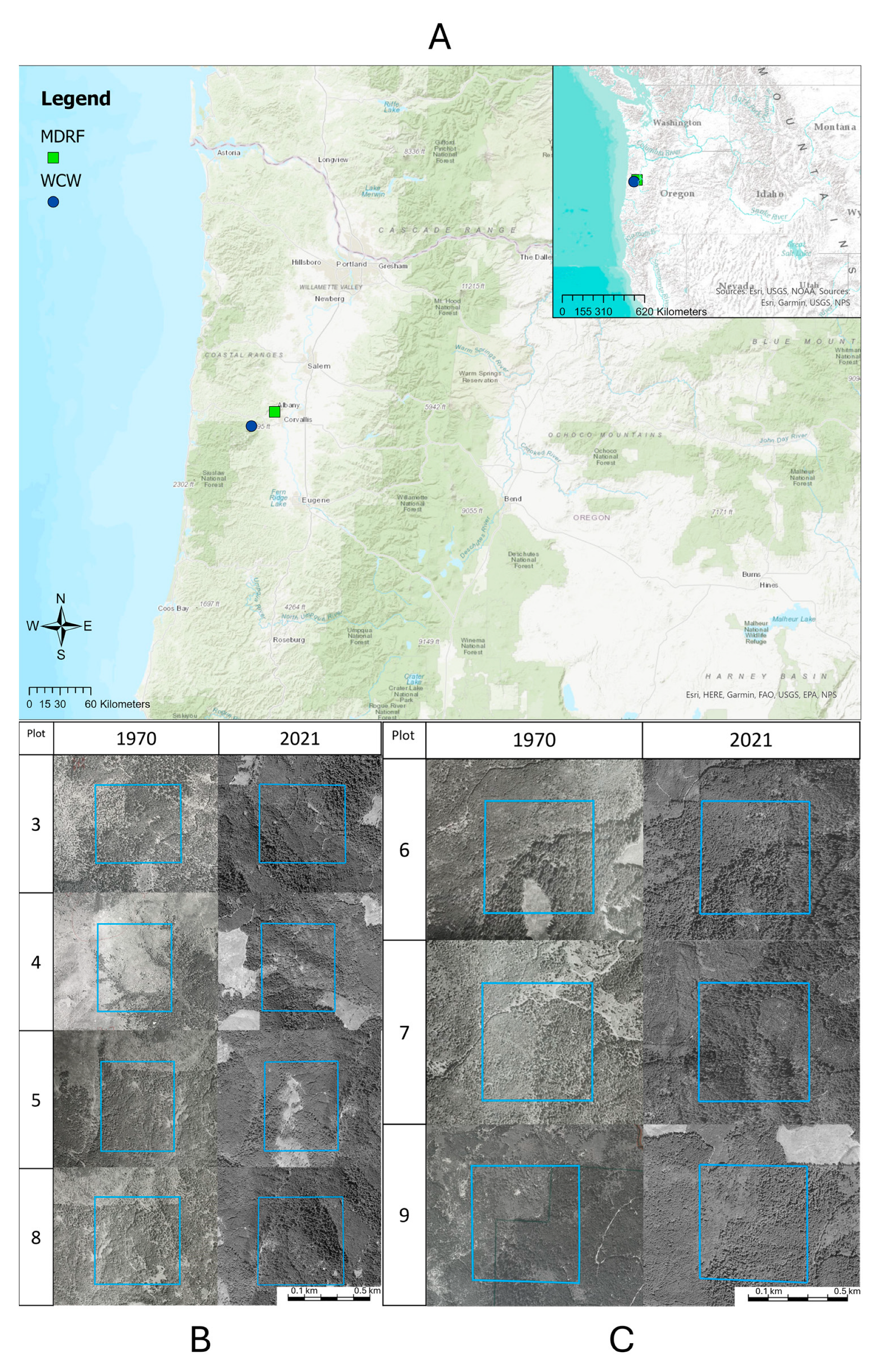
2.1. Study Site and Historical Surveys

From 1968 through 1970, Stanley Anderson surveyed the bird and plant communities of the Coast Range Mountains within 20 km of Corvallis, Oregon, USA (Figure 1A). Anderson’s goal was to classify seasonal changes in the diversity and ecological structure of local avifauna in Douglas-fir (Pseudotsuga menziesii)-dominated forests [29,30]. His effort was the first in this ecosystem to produce quantitative estimates of bird abundance. To do this, Anderson non-randomly selected 10 forested study plots in Oregon State University’s McDonald-Dunn Research Forest (MDRF) (Figure 1B) and the Woods Creek Watershed (WCW) (Figure 1C) portion of the Siuslaw National Forest in Benton County, Oregon, USA [29,30]. Anderson’s original plots (quarter sections, each one quarter mile by one quarter mile, or 64.8 ha) were identified based on the U.S. Public Land Survey System information (township, range, section, and quarter section) and were named in a numeric sequence (plots 1–10); he did not describe specifically which areas within the quarter sections were surveyed.
Anderson counted birds using a sample count method in which he conducted 10 min stationary point counts spaced approximately 95 m apart along an irregular transect that followed roads or trails. During each survey, Anderson recorded all birds seen within 18 m, and if a bird was heard, he attempted to locate it; heard-only birds were apparently not counted [29,30]. Surveys were conducted on good weather days starting one hour after sunrise at least once per week between early June and mid-July, 1968–1970. Anderson reported his count results as the density per 40.5 ha (100 acres) for each species in each plot; no confidence intervals or other statistical measures of error were reported. Original data were not archived. Anderson also measured several vegetation structure characteristics within each plot by following a transect sampling method outlined in Cottam and Curtis (1956) [31]; these included trees per acre, height class distribution, shrub density, and qualitative descriptions of vegetation for each plot.

2.2. Modern Study Site and Surveys

We selected seven of Anderson’s original ten conifer-dominated plots; three plots were excluded because they had been recently altered by forest harvest practices (clear cut) or were not primarily coniferous forest. During our surveys, the four plots in MDRF (plots 3, 4, 5, and 8) were dominated by Douglas-fir and big leaf maple (Acer macrophyllum) and had experienced a relatively high rate of timber harvest in the last 50 years, resulting in a mosaic of forest ages (based on qualitative assessment of aerial imagery; Figure 1B). The three plots in WCW (plots 6, 7, and 9), composed of relatively even-aged Douglas-fir and small patches of western hemlock (Tsuga heterophylla), were mostly undisturbed in the last 50 years (Figure 1C). We conducted our surveys within the quarter sections and assumed, because we were surveying the same habitats, that our density estimates would be reliably comparable to Anderson’s. Reduced access to plots 6 and 7 due to COVID-19-related restrictions resulted in multiple counts that were conducted near the boundaries of the quarter sections (within 250 m) but in the same habitats as those within the plots. We categorized the surveys as “In” or “Out” of quarter sections to assess any potential differences in avian communities; we found no consistent differences and combined all of the surveys for the analyses [22].
To ensure our results were comparable to Anderson’s, we mimicked his bird survey methods as closely as possible by conducting 10 min stationary point counts spaced approximately 100 m apart along roads and trails. Each plot was surveyed twice each year (2020 and 2021), usually once by each skilled observer (NMC and WDR), between dawn and five hours after sunrise on days with little or no rain or wind. We implemented modern counting methods using unlimited radius count areas and recording distance to (checked with a laser rangefinder) and detection type (singing, calling, visual, flyover, and drumming) for each bird [32]. Following Anderson’s survey protocol, if a bird was heard within 18 m, we made an attempt to visually locate it. Thus, we repeated Anderson’s avian survey methodology as closely as possible while also using modern survey techniques and preserving extensive metadata to better facilitate future resurveys and analyses [32].

2.3. Landscape and Habitat Comparison

We measured vegetation with a method that produced results directly comparable to the method used by Anderson. The James and Shugart (1970) [33] approach generates calculations of shrubs and trees per hectare more efficiently. Employing their method, we sampled vegetation structure in 70 randomly selected 12 m radius circular plots (10 in each of Anderson’s seven plots). We then identified the species and diameter at breast height category of each tree and counted the number of shrubs over 1 m tall in a 2 m wide swath along north–south and east–west transects through the diameter of each circular plot. We also visually compared orthographic aerial photographs from 1970 to Landsat satellite imagery from 2021 to characterize broad, landscape-level habitat changes. Finally, we overlaid grids across landscape imagery from both time periods to estimate the percent of total area harvested and change in forest and clearcut cover between 1968 and 2021 for each plot.

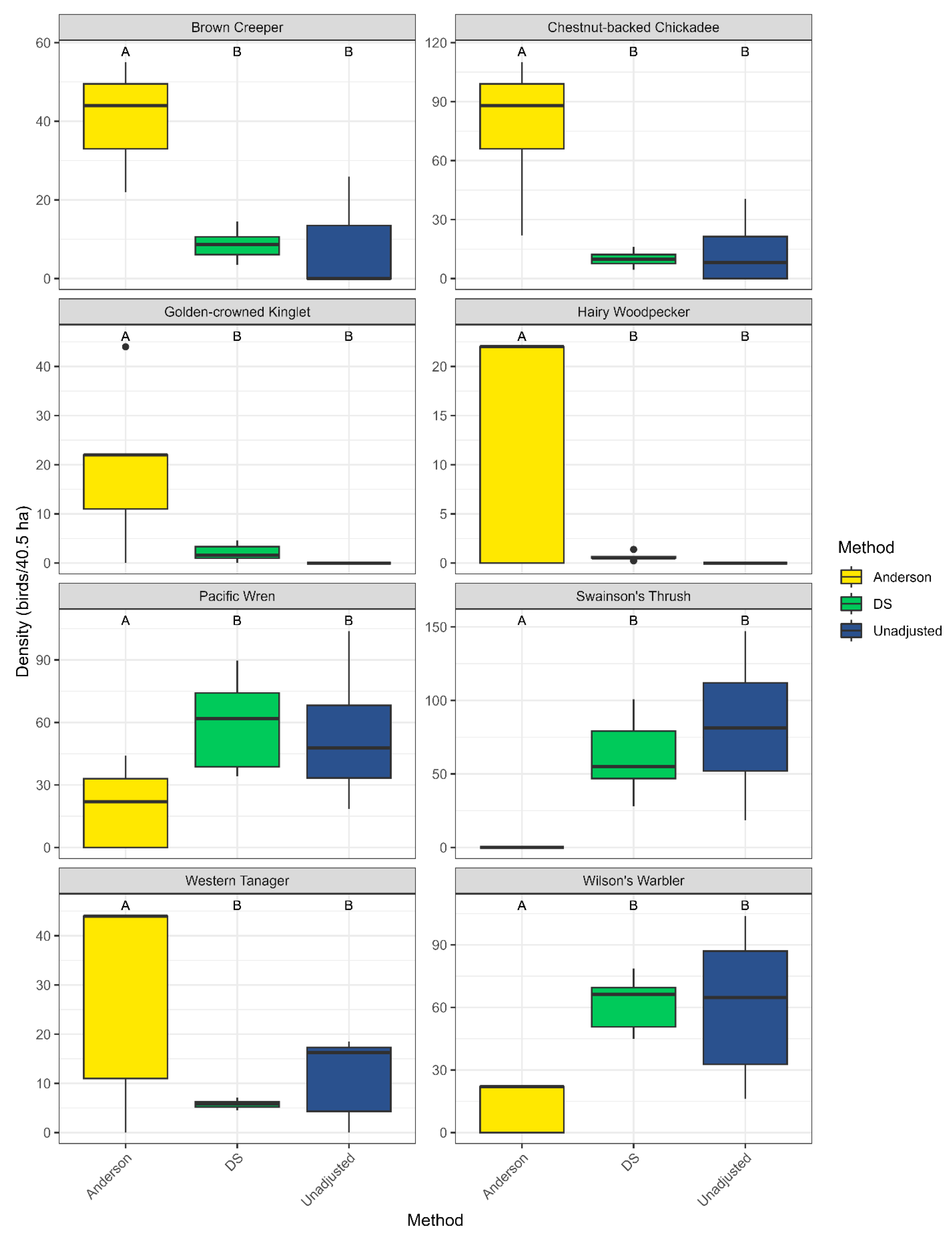
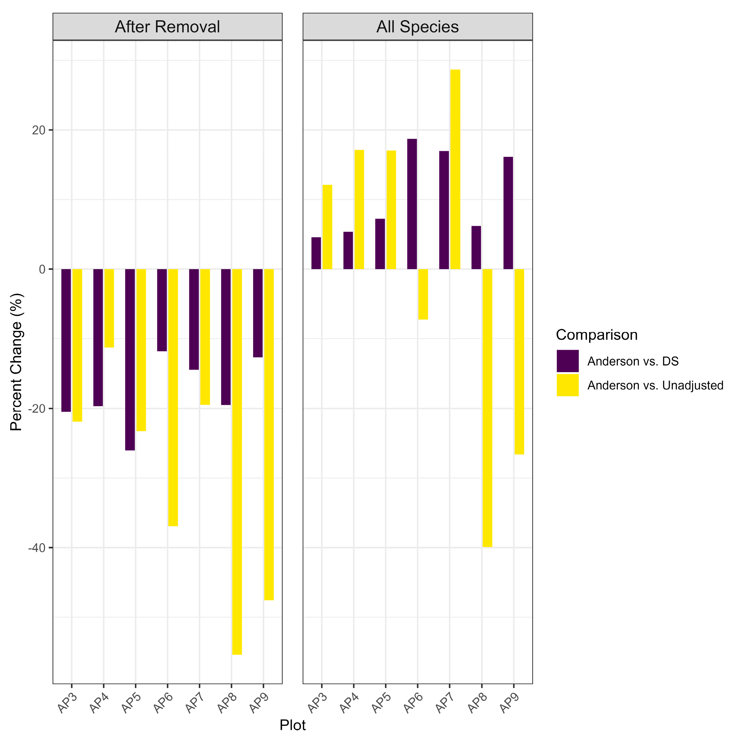
2.4. Density Estimation and Comparison

We estimated density in two ways: one method mirrored Anderson’s method by simply calculating the density of birds observed within 18 m (hereafter referred to as the unadjusted method as it was not adjusted from Anderson’s original method nor did it employ adjustments for detectability); the second method incorporated distance sampling to provide density estimates which account for imperfect detectability [34]. By estimating density using these two methods, we present directly comparable estimates and also preserve estimates which account for detectability differences across species, provide errors of estimation, and may be more useful when surveys are replicated in the future. Distance sampling was only applied to species with greater than 10 total detections. For 25 species, we used detection key functions established by a regional benchmark survey which has hundreds to thousands of detections for each species produced from unlimited radius point counts, the majority of which were generated by WDR [35] (Table S1). If a detection model encountered errors associated with monotonicity violations or the total number of observations in our dataset was insufficient to allow for the application of previously established key functions (true for 16 species), we performed backwards parameter selection using Akaike information criterion to select the most appropriate key function (Table S1). Additionally, 15 rare species had fewer than 10 observations, and none were detected within 18 m. Because those species were not reported by Anderson at all, we omitted those species from further efforts to estimate their densities.
To assess species-specific differences in density for Anderson’s era and ours, we treated each plot as a replicate for each species and performed analysis of variance tests, with Tukey’s honestly significant difference post hoc test to adjust for multiple comparisons. To detect potential signals of habitat change at the plot level, we also summed density estimates across all species for each plot and then subtracted combined modern estimates from Anderson’s. We then converted the differences to percent change to allow for between-plot comparisons. Density estimation and statistical analyses were all conducted in R [36] and the Distance package [37].
We compared these results with BBS abundance trends from statewide surveys and routes within 80 km of Anderson’s plots, in similar habitats, and with greater than 30 years of data in the last half century; only two BBS routes, Salado (69009) and Elkton (69050), meet those criteria. BBS trends were produced by Sauer et al. (2020) [38], who used hierarchical models to calculate changes in annual indices of abundance. We simplified BBS results by categorizing trend coefficients into three categories: declining (<−0.50), stable (−0.50–0.50), and increasing (>0.50). We then simplified our results into similar categories: if both unadjusted and distance sampling estimates were statistically different from Anderson’s, we considered those species declining or increasing depending on the directionality of the change. If only one or neither of the modern estimates were statistically different from Anderson’s, we considered those species’ abundances to be stable.
Finally, we assessed relationships between changes in habitat and bird densities by modeling differences in densities as a function of plot-specific changes vegetation and landscape characteristics for each species. We ran two sets of linear models using plots as replicates (n= 6 for each species): one with changes in bird density as the difference between unadjusted and Anderson’s estimates, and another with distance sampling estimates in the place of unadjusted. Vegetation and landscape covariates were derived from the efforts described above.

3. Results

3.1. Avian Communities

We conducted 304 stationary (point) counts in June 2020 and 2021, recording 4203 birds of 64 species of which 391 birds and 35 species were observed within 18 m. Five species were observed within 18 m in all plots: Swainson’s Thrush (Catharus ustulatus) (n = 388), Wilson’s Warbler (Cardellina pusilla) (n = 368), Hermit Warbler (Setophaga occidentalis) (n = 360), Pacific Wren (Troglodytes pacificus) (n = 339), and Western Flycatcher (Empidonax difficilis) (n = 301) (Table 1 and Table S1). Those five species accounted for 41.8% of the total observations.
Distance sampling produced density estimates for 39 species, while our unadjusted method produced estimates for 35 species (Table 2). At a landscape scale (when all plots were combined), distance sampling and unadjusted density estimates were significantly different for only three species: Red-breasted Sapsucker (Sphyrapicus ruber), Red Crossbill (Loxia curvirostra), and Common Raven (Corvus corax) (p < 0.001 for all three species). Each of those species was rarely encountered within 18 m (Table S2).
We observed a similar number of total species within 18 m radius counts as Anderson; however, some variability existed among the plots (Table 2). Within 18 m, species unique to each era numbered 13 in Anderson’s surveys and 14 in ours (Table S3). Of the 13 species detected by Anderson that we missed on the 18 m surveys, we detected 10 of them in our unlimited-radius counts. Thus, Anderson found only 3 species that we did not detect.
For seven species, both of our density estimates were significantly different from Anderson’s: Hairy Woodpecker (Dryobates villosus), Chestnut-backed Chickadee (Poecile rufescens), Brown Creeper (Certhia americana), Pacific Wren, Golden-crowned Kinglet (Regulus satrapa), Swainson’s Thrush, Wilson’s Warbler, and Western Tanager (Piranga ludoviciana) (Table S2, Figure 2). Of these, we found higher densities for three (Wilson’s Warbler, Swainson’s Thrush, and Pacific Wren); the remainder were all found to have lower densities (Figure 2). We observed non-significant differences in the densities of 33 species (Table S2).
Differences in the total bird density between historical and modern estimates were highly variable across the plots and methods of estimation (Figure 3). Results from three species (Swainson’s Thrush, Wilson’s Warbler, and Orange-crowned Warbler (Leiothlypis celata)) in the modern surveys contributed strongly to this pattern and collectively accounted for more than 40% of the overall change in densities. Each of those three species were abundant and omnipresent during our surveys but were absent or present in only small numbers in Anderson’s surveys. When we compared changes in total bird abundance without those species, changes in density were consistent between the survey eras (Figure 3).

3.2. Comparisons with BBS Data

BBS data revealed that most species were declining at the state-wide level, but most were stable on the two Coast Range survey routes. At the state level, 53.8% of species considered here were declining, 9.4% were increasing, and 30.8% were stable. The two local BBS routes, Elkton and Salado, had 36.8% declining, 5.3% increasing, and 57.9% stable and 8.1% declining, 35.1% increasing, and 56.8% stable, respectively. Our surveys from Anderson’s plots indicated 12.8% declining, 7.7% increasing, and 79.5% stable. In only four species did all the sources produce similar trends (Hammond’s Flycatcher (Empidonax hammondii), Red-breasted Nuthatch (Sitta canadensis), Varied Thrush (Ixoreus naevius), and Pine Siskin (Spinus pinus)), of which all were observed to have stable trends. Similarly, 7 species were either increasing or stable at local BBS routes and in our comparisons with Anderson’s data, but declining at the state level (Figure 4).

3.3. Habitat Change at Plot and Landscape Levels

Over the 50 years between bird surveys, timber harvest activities, including thinning, shelter cuts, or clear cuts, occurred in five of seven plots. The habitat changes occurred disproportionately in MDRF (all plots) as compared with WCW (only plot 7). Plot 5 experienced the greatest change, with >70% of the forest harvested, while forest management in plots 3 and 7 impacted less than 30% of each plot (Table 3). Generally, forest cover was higher in 2021 than in 1970, with aerial photographs showing evidence of forest maturation into mid-successional stages (Table 3, Figure 1B,C). Forest cover generally increased across the landscape, with most plots experiencing an increase of 5–10%; clearcut cover decreased by similar magnitudes. However, in plot 4, there was a >75% increase in forest cover that coincided with an 80% decrease in clearcut cover. This harvest occurred within a year after Anderson conducted his surveys; we were able to find aerial photographs of this sector within 5 years of when Anderson’s research was conducted. Consistent with this landscape pattern of general forest succession, we observed a lower shrub density in all the plots and increased density of live trees in most plots. Vegetation species composition was mostly consistent across all plots. The understory was dominated by vine maple (Acer circinatum) in most plots, and Douglas-fir was the most abundant tree, followed by grand fir (Abies grandis) and western hemlock (Tsuga heterophylla) in WCW plots [22].

3.4. Correlations Between Changes in Habitat and Bird Density

Changes in bird densities were not consistently explained by changes in vegetation structure or landscape cover composition. Of the eight species for which we found significant changes in density, only two (Pacific Wren and Chestnut-backed Chickadee) had statistically significant (p < 0.05) coefficients. Similarly, only one (MacGillivray’s Warbler (Geothylpis tolmiei)) of the five species with relevant habitat requirements (Hermit Warbler, Orange-crowned Warbler, White-crowned Sparrow (Zonotrichia leucophrys), and Willow Flycatcher (Empidonax traillii)) had statistically significant coefficients. Of the 27 additional species considered in this section of the analysis, only 4 had at least 1 statistically significant coefficient (American Robin (Turdus migratorius), Hammond’s Flycatcher, Mourning Dove (Zenaida macroura), and Red Crossbill (Loxia curvirostra)) (Table S4). Among the seven species with significant coefficients, there were no consistent patterns in parameters or coefficient directionality. Regardless of significance, for nearly all the species, coefficients for both change in clearcut and forest cover were large across most species, in comparison to those of change in tree and shrub density.

4. Discussion

Comparing two snapshot surveys conducted 50 years apart in a Pacific Northwest bird community, we found 80% of breeding bird species to have statistically similar abundances. Despite active forest management across the landscape, relative stability in bird populations was the common pattern. We documented significant declines in only five species, contrary to other studies reporting losses of many North American woodland passerines over similar time periods. Furthermore, we observed no common patterns associated with foraging guilds among the species which experienced significant changes in density. The local plot-level patterns were generally mirrored by regional trends but less correlated with state-level trends derived from the BBS. Furthermore, we detected few unambiguous relationships between anthropogenic change in habitat and densities of breeding bird species. Our study not only highlights the utility of historical datasets in detecting community change in areas not surveyed by large-scale efforts such as the BBS, but also demonstrates the need for the thorough documentation and preservation of avian benchmark data. We preserve extensive data, metadata, and details on methodology here and in [32] to facilitate more precise replication during future resurveys.
We capitalized on the level of detail preserved in Anderson’s thesis, which is comparatively rich for its period, by resurveying the same plots and directly comparing estimates of density from across the study area to maintain consistency in comparisons across time periods. We believe that only minor differences in methodology existed between our and Anderson’s work. Nevertheless, some odd results from Anderson’s surveys have constrained our conclusions. For instance, Anderson reported no density estimates for Swainson’s Thrush, the most abundant species during our surveys. This absence is not easily explained. The probability of detection in close proximity is high as the species sings often and can be seen regularly as it commonly nests in the understory. We saw no evidence in Anderson’s data that an identification error may have occurred, such as confusion with Hermit Thrush, a species more numerous at much higher elevations. Furthermore, BBS results suggest Swainson’s Thrush was present and common in the region during Anderson’s era. A possible explanation for the absence of Swainson’s Thrush in Anderson’s data is a clerical error which occurred in the process of manuscript transcription. We therefore treat the statistically significant change observed for that species with caution. Despite the odd lack of Swainson’s Thrushes in Anderson’s data, density estimates for all other species appear realistic.
Modern bird counting methods focus on evaluating the important influences of detectability on abundance estimates. The use of density estimation methods that do not account for the imperfect detectability of birds can be prone to underestimation [34], and thus estimates of density and abundance from historical datasets may not be entirely accurate [18]. Yet, using identical methods to those from historic surveys, pre-dating the development of protocols to adjust for detectability challenges, can still reveal important biological changes [40,41,42]. To assess the accuracy of unadjusted density estimation methods, we estimated density using an identical method to Anderson, and we also incorporated distance sampling to provide more accurate and replicable density estimates. We observed no consistent differences between these methods, except for three wide-ranging species rarely detected near observers. While Anderson’s methodology may not have produced estimates that account for detectability as modern methods do, they did appear to capture realistic patterns in the densities across this bird community.
Despite our efforts to replicate Anderson’s surveys as precisely as possible and provide well-reasoned statistical comparisons, we observed large variability in density estimates for some species. Unadjusted density estimates were highly variable across all the plots for species which range widely or that exist on the landscape at inherently low densities, and therefore are detected infrequently in close proximities to the observer. Furthermore, distance sampling methods produced large estimates of variation for some species. When we also consider the inherent uncertainty of Anderson’s density estimates without the original data, the power with which we can draw reliable conclusions is low. However, for easily detected species consistently encountered in close proximity to observers, we believe that our analysis captures broad, but accurate patterns for these species.

4.1. Local and Regional Change in Avian Communities

Several publications have published analyses describing declines in some segments of the North American avifauna in the last half century, particularly in forest bird communities [5,43,44]. In contrast, our results reveal that most species in our study have densities similar to those of the late 1960s. At the state-wide level, Oregon BBS trends show declines for a majority of the species considered in our study [38]. However, this statewide pattern is not evident in BBS data from routes within 80 km that surveyed habitats most similar to those in our study plots. BBS results indicate less than 35% of species experienced declines on a regional level, in comparison to approximately 80% on a state level. Notably, Pacific Wren, Western Flycatcher, Western Wood-Pewee (Contopus sordidulus), Wilson’s Warbler, and Black-throated Gray Warbler (Setophaga nigrescens) have increased in the Coast Range region but decreased across Oregon. For only one species, Red-breasted Sapsucker (Sphyrapicus ruber), was there an increase at the state level but a decline regionally. A majority of the remaining species were declining at the state level and stable regionally.
Results from our study generally align with those from local BBS data. We observed similar declines in Brown Creeper, Chestnut-backed Chickadee, and Golden-crowned Kinglet, and increases in Pacific Wren and Wilson’s Warbler, which suggests our observed changes for these species are not isolated to Anderson’s plots and may reflect patterns of change in density for the central Oregon Coast Range. Of these species, only Wilson’s Warbler is declining on a state and continental scale [5,38]. North American declines of Wilson’s Warbler are attributed mainly to loss of breeding habitat [45], but the perpetuation of early to mid-seral forests, the preferred breeding of Pacific Northwest populations [46], by forest harvest practices may be the cause for regionally increasing populations.
One other study in western Oregon resurveyed a historic set of study plots to evaluate changes in avian community composition [26,27], providing substantial evidence for community turnover. Curtis et al. (2016) found that community shifts were not associated with changes in habitat, rather that the natural dynamism of avian communities resulted in significantly different species composition but similar overall abundances of birds in each community through time. We did not conduct community ordination analyses but observed more than 70% overlap in species composition between our snapshots, suggesting the level of species turnover was lower in our study area.

4.2. Avian Response to Agricultural Forests

A few previous resurvey studies have used complex analytical methods to model changes in bird communities and habitat [24,27]. Our ability to understand the effect sizes of habitat variables was constrained given the small sample size available (six density estimates/species). We employed a simple approach that involved applying basic linear models to assess statistical relationships of change in bird density and habitat characteristics. Most species had statistically ambiguous relationships with changes in vegetation structure and landscape cover. Where these were significant, the effect sizes were largest for changes in landscape cover, as opposed to vegetation structure or harvest acreage.
Habitat availability influences population dynamics and persistence and specific components of a habitat can strongly influence bird occurrence and abundance [44,47,48]. Where tracts of suitable habitat exist, species experiencing declines at broader spatial scales may persist locally if important single habitat features (e.g., a large, hollow snag) are present or if species-specific patch sizes of habitat are available [49,50]. This may suggest that the patterns observed in our study deviating from state-level BBS trends reflect the presence or absence of habitat characteristics we were unable to measure. We found no clear evidence that changes in habitat characteristics within the study area were a consistent driver of changes in bird density. However, the constraints of the small sample size of plots and limitations of the habitat and landscape cover data may impact the comparisons.
Subtle changes in habitat availability may have occurred within our study area that are not easily quantified from historic aerial photographs or the preserved vegetation information in Anderson’s original work. For instance, standing dead tree removal was a common forest management practice in the Pacific Northwest until the 1980s, when their ecological importance was prioritized [51]. Chambers et al. (1997) [52] artificially created snags in the vicinity of two of Anderson’s original plots, but these efforts have not been replicated on a landscape level. Coincidently, of the five species we found to have significantly reduced densities since the 1950s, three (Hairy Woodpecker, Brown Creeper, and Chestnut-backed Chickadee) have some ecological association with standing dead trees, and another species highly dependent on snags during breeding season (Vaux’s Swift (Chaetura vauxi) was present in Anderson’s surveys but absent on ours. Without data on the density of standing dead trees across our study area, we cannot definitively link the observed declines to snag removal; however, it is possible that the systematic removal of such features over the 20th century could contribute to the decline of certain species.
We summed density across all the species in each plot in an effort to detect plot-specific patterns which may reflect significant habitat changes. We found that two species (Wilson’s Warbler and Orange-crowned Warbler) accounted for more than 20% of the overall change. This is partly because Anderson detected comparatively few individuals of these species, whereas these were among the most frequently observed species in our surveys. Comparisons of percent change in total density prior to the removal of the species from the analysis show consistent increases across nearly all the plots, whereas, after the removal of these species, patterns are opposite. Notably, the plots showing the smallest change (whether that be positive in comparisons pre-removal, or negative post-removal) were also the plots to have experienced the most anthropogenic habitat alteration. In contrast, plots that seemingly experienced consistent, undisturbed maturation into mid-seral stages exhibited stronger declines in density. This aligns with the intermediate disturbance hypothesis and previously observed bimodal patterns of avian richness and abundance in coniferous forest, in which these metrics peak in early and late seral stages but regress in mid stages [53,54].

5. Conclusions

By comparing two snapshots of avian communities separated by 50 years, we document general stability in the density of approximately 80% of the species of conifer woodland birds in our study area. This pattern appears generally consistent for the Central Oregon Coast Range, based on similar observations from regional BBS results. While many species have maintained relatively stable abundances through time, ongoing shifts in highly dynamic agricultural forests have the potential to drive more pronounced changes for species with specific habitat requirements.
While Anderson’s bird surveys have enabled us to quantify temporal changes in avian density and their association with dynamics in agricultural forests, the shortcomings of historical survey methods and incomplete data preservation highlight the need for highly detailed community benchmark surveys with the archival of detailed metadata to facilitate future analyses of change. Effectively preserved snapshots of avian communities allow for precisely repeatable resurveys and rigorous analyses, which ultimately result in highly informative conclusions [35,55]. In the few cases in which historical snapshots are preserved in enough detail to allow for highly repeatable resurvey efforts, the results can better evaluate ecological theory and support conservation action (e.g., Ellis et al. 2019). Unfortunately, with the passage of time, boxes of old notebooks and data are lost, and investigators driven enough to interpret results from outdated survey methods or to carefully evaluate partial datasets are tasked with surmounting many hurdles that historical datasets present. Carefully gauged analyses and interpretation can still provide insights about long-term change in bird communities even when historic approaches have been replaced by better methods (e.g., Robinson 1999, Tingley and Beissinger 2009). We join others [19,26,56,57] arguing that historical datasets are not a lost cause, but instead can provide useful insights into long-term changes as long as the interpretation of results is evaluated judiciously.

Supplementary Materials

The following supporting information can be downloaded at https://www.mdpi.com/article/10.3390/d17020123/s1: Table S1. Distance sampling parameters for species with greater than 10 observations with associated AIC of the selected detection function and sample size. Functions were retained if the a priori model from Robinson et al. (2020) [35] did not encounter errors; where errors related to violations of monotonicity or sample size occurred, a new detection function was chosen using backward AIC selection. We present both the original and the selected key functions in case they differ and to preserve methodological detail. Taxonomic names and sequence follow the American Ornithological Society [39]; Table S2. P-values from Tukey’s honestly significant difference post hoc test for comparing density estimates from Distance Sample (DS), Unadjusted (based on birds observed within 18 m), and Anderson’s original estimates; Table S3. List of species observed within 18 m unique to only one snapshot. Taxonomic names and sequence follow the American Ornithological Society [39]; Table S4. Output from linear models to assess correlations between changes in bird density and changes in vegetation and landscape characteristics for 17 species: the eight focal species with significant changes in density (*), four species with relevant habitat associations (^), and five species with changes in density that were significantly related to at least one habitat or landscape covariate (+). The 32 other species considered in this analysis did not have significant relationships between change in density and habitat or landscape variables, so are not included here; Table S5. Output from Distance Sampling models for all species with greater than 10 total detections. Models were run using the Distance Package in R [36,37].

Author Contributions

Conceptualization, N.M.C. and W.D.R.; methodology, N.M.C., F.-Y.S., and W.D.R.; formal analysis, N.M.C. and F.-Y.S.; writing, N.M.C., F.-Y.S., and W.D.R.; and funding acquisition, W.D.R. All authors have read and agreed to the published version of the manuscript.

Funding

This research was funded by the Bob and Phyllis Mace Professorship and Hatch Funds (W.D.R.).

Institutional Review Board Statement

Not applicable.

Data Availability Statement

The raw data supporting the conclusions of this article will be made available by the authors on request.

Acknowledgments

We thank Brent Klumph and Steve Fitzgerald of Oregon State University College of Forestry for the permission to access the McDonald-Dunn Research Forest. Similarly, we thank Starker Forests, Inc., for permitting us to conduct surveys on their property adjacent to the Siuslaw National Forest. Thank you to Rachel Lilley with the Oregon State University Special Collections and Archives Research Center and Kathy Stroud with the University of Oregon Library for facilitating access to historic aerial photography. We thank two anonymous reviewers for their helpful and constructive feedback on the manuscript.

Conflicts of Interest

The authors declare no conflicts of interest. The funders had no role in the design of the study; in the collection, analyses, or interpretation of data; in the writing of the manuscript; or in the decision to publish the results.

Abbreviations

The following abbreviations are used in this manuscript:
BBSUSGS Breeding Bird Survey
MDRFMcDonald-Dunn Research Forest
WCWWoods Creek Watershed

References

  1. Wiens, J.A.; Stralberg, D.; Jongsomjit, D.; Howell, C.A.; Snyder, M.A. Niches, Models, and Climate Change: Assessing the Assumptions and Uncertainties. Proc. Natl. Acad. Sci. USA 2009, 106, 19729–19736. [Google Scholar] [CrossRef]
  2. Temple, S.; Wiens, J. Bird Populations and Environmental Changes: Can Birds Be Bio-Indicators? Am. Birds 1989, 43, 260–270. [Google Scholar]
  3. Crick, H.Q.P. The Impact of Climate Change on Birds. Ibis 2004, 146, 48–56. [Google Scholar] [CrossRef]
  4. Phalan, B.T.; Northrup, J.M.; Yang, Z.; Deal, R.L.; Rousseau, J.S.; Spies, T.A.; Betts, M.G. Impacts of the Northwest Forest Plan on Forest Composition and Bird Populations. Proc. Natl. Acad. Sci. USA 2019, 116, 3322–3327. [Google Scholar] [CrossRef]
  5. Rosenberg, K.V.; Dokter, A.M.; Blancher, P.J.; Sauer, J.R.; Smith, A.C.; Smith, P.A.; Stanton, J.C.; Panjabi, A.; Helft, L.; Parr, M.; et al. Decline of the North American Avifauna. Science 2019, 366, 120–124. [Google Scholar] [CrossRef] [PubMed]
  6. Swanson, F.J.; Franklin, J.F. New Forestry Principles from Ecosystem Analysis of Pacific Northwest Forests. Ecol. Appl. 1992, 2, 262–274. [Google Scholar] [CrossRef] [PubMed]
  7. Kennedy, R.S.H.; Spies, T.A. Forest Cover Changes in the Oregon Coast Range from 1939 to 1993. For. Ecol. Manag. 2004, 200, 129–147. [Google Scholar] [CrossRef]
  8. McGarigal, K.; McComb, W.C. Relationships Between Landscape Structure and Breeding Birds in the Oregon Coast Range. Ecol. Monogr. 1995, 65, 235–260. [Google Scholar] [CrossRef]
  9. Betts, M.G.; Hagar, J.C.; Rivers, J.W.; Alexander, J.D.; McGarigal, K.; McComb, B.C. Thresholds in Forest Bird Occurrence as a Function of the Amount of Early-Seral Broadleaf Forest at Landscape Scales. Ecol. Appl. 2010, 20, 2116–2130. [Google Scholar] [CrossRef]
  10. Harris, S.H.; Betts, M.G. Bird Abundance Is Highly Dynamic across Succession in Early Seral Tree Plantations. For. Ecol. Manag. 2021, 483, 118902. [Google Scholar] [CrossRef]
  11. Ellis, T.M.; Betts, M.G. Bird Abundance and Diversity across a Hardwood Gradient within Early Seral Plantation Forest. For. Ecol. Manag. 2011, 261, 1372–1381. [Google Scholar] [CrossRef]
  12. Cahall, R.E.; Hayes, J.P.; Betts, M.G. Will They Come? Long-Term Response by Forest Birds to Experimental Thinning Supports the “Field of Dreams” Hypothesis. For. Ecol. Manag. 2013, 304, 137–149. [Google Scholar] [CrossRef]
  13. Rivers, J.W.; Verschuyl, J.; Schwarz, C.J.; Kroll, A.J.; Betts, M.G. No Evidence of a Demographic Response to Experimental Herbicide Treatments by the White-Crowned Sparrow, an Early Successional Forest Songbird. Condor 2019, 121, duz004. [Google Scholar] [CrossRef]
  14. Sallabanks, R.; Arnett, E.B.; Marzluff, J.M. An Evaluation of Research on the Effects of Timber Harvest on Bird Populations. Wildl. Soc. Bull. 2000, 28, 1144–1155. [Google Scholar]
  15. Vanderwel, M.C.; Malcolm, J.R.; Mills, S.C. A Meta-Analysis of Bird Responses to Uniform Partial Harvesting across North America. Conserv. Biol. 2007, 21, 1230–1240. [Google Scholar] [CrossRef]
  16. Link, W.A.; Sauer, J.R. Estimating Population Change from Count Data: Application to the North American Breeding Bird Survey. Ecol. Appl. 1998, 8, 258–268. [Google Scholar] [CrossRef]
  17. Magurran, A.E.; Baillie, S.R.; Buckland, S.T.; Dick, J.M.; Elston, D.A.; Scott, E.M.; Smith, R.I.; Somerfield, P.J.; Watt, A.D. Long-Term Datasets in Biodiversity Research and Monitoring: Assessing Change in Ecological Communities through Time. Trends Ecol. Evol. 2010, 25, 574–582. [Google Scholar] [CrossRef]
  18. Igl, L.D.; Johnson, D.H. A Retrospective Perspective: Evaluating Population Changes by Repeating Historic Bird Surveys. USDA For. Serv. Gen. Tech. Rep. 2005, PSW-GTR-191, 817–830. [Google Scholar]
  19. Tingley, M.W. Turning Oranges into Apples: Using Detectability Correction and Bias Heuristics to Compare Imperfectly Repeated Observations. In Stepping in the Same River Twice: Replication in Biological Research; Yale University Press: London, UK, 2017; pp. 215–233. [Google Scholar]
  20. Robinson, W.D. Long-Term Changes in the Avifauna of Barro Colorado Island, Panama, a Tropical Forest Isolate. Conserv. Biol. 1999, 13, 85–97. [Google Scholar] [CrossRef]
  21. Iknayan, K.J.; Beissinger, S.R. Collapse of a Desert Bird Community over the Past Century Driven by Climate Change. Proc. Natl. Acad. Sci. USA 2018, 115, 8597–8602. [Google Scholar] [CrossRef] [PubMed]
  22. Clements, N.M.; Robinson, W.D. A Comparison of Two Snapshot Studies Half a Century Apart Suggests Stability in a Pacific Northwest Winter Forest Bird Community. Front. Bird Sci. 2024, 3, 1304026. [Google Scholar] [CrossRef]
  23. Tingley, M.W.; Beissinger, S.R. Detecting Range Shifts from Historical Species Occurrences: New Perspectives on Old Data. Trends Ecol. Evol. 2009, 24, 625–633. [Google Scholar] [CrossRef] [PubMed]
  24. Tingley, M.W.; Monahan, W.B.; Beissinger, S.R.; Moritz, C. Birds Track Their Grinnellian Niche through a Century of Climate Change. Proc. Natl. Acad. Sci. USA 2009, 106, 19637–19643. [Google Scholar] [CrossRef] [PubMed]
  25. Tingley, M.W.; Beissinger, S.R. Cryptic Loss of Montane Avian Richness and High Community Turnover over 100 Years. Ecology 2013, 94, 598–609. [Google Scholar] [CrossRef] [PubMed]
  26. Curtis, J.R.; Robinson, W.D. Sixty Years of Change in Avian Communities of the Pacific Northwest. PeerJ 2015, 3, e1152. [Google Scholar] [CrossRef]
  27. Curtis, J.R.; Robinson, W.D.; McCune, B. Time Trumps Habitat in the Dynamics of an Avian Community. Ecosphere 2016, 7, e01575. [Google Scholar] [CrossRef]
  28. Ellis, M.S.; Kennedy, P.L.; Edge, W.D.; Sanders, T.A. Twenty-Year Changes in Riparian Bird Communities of East-Central Oregon. Wilson J. Ornithol. 2019, 131, 43–61. [Google Scholar] [CrossRef]
  29. Anderson, S.H. Ecological Relationships of Birds in Forest of Western Oregon; Oregon State University: Corvallis, OR, USA, 1970. [Google Scholar]
  30. Anderson, S.H. Seasonal Variations in Forest Birds of Western Oregon. Northwest Sci. 1972, 46, 194–206. [Google Scholar]
  31. Cottam, G.; Curtis, J.T. The Use of Distance Measures in Phytosociological Sampling. Ecology 1956, 37, 451–460. [Google Scholar] [CrossRef]
  32. Clements, N.; Robinson, W. A Re-Survey in 2019-2021 of Winter Bird Communities in the Oregon Coast Range, USA, Initially Surveyed in 1968–1970. Biodivers. Data J. 2022, 10, e91511. [Google Scholar] [CrossRef] [PubMed]
  33. James, F.C.; Shugart, H.H. A Quantitative Method of Habitat Description. Audubon Field Notes 1970, 24, 727–736. [Google Scholar]
  34. Buckland, S.T.; Anderson, D.R.; Burnham, K.P.; Laake, J.L.; Borchers, D.L.; Thomas, L. Introduction to Distance Sample: Estimating Abundance of Biological Populations; Oxford University Press: New York, NY, USA, 2001. [Google Scholar]
  35. Robinson, W.D.; Hallman, T.A.; Curtis, J.R. Benchmarking the Avian Diversity of Oregon in an Era of Rapid Change. Northwestern Nat. 2020, 101, 180–193. [Google Scholar] [CrossRef]
  36. R Core Team. R: A Language and Environment for Statistical Computing; Foundation for Statistical Computing: Vienna, Austria, 2021. [Google Scholar]
  37. Thomas, L.; Buckland, S.T.; Rexstad, E.; Laake, J.L.; Strindberg, S.; Hedley, S.L.; Bishop, J.R.B.; Marques, T.A. Distance Software: Design and Analysis of Distance Sampling Surveys for Estimating Population Size. J. Appl. Ecol. 2010, 47, 5–14. [Google Scholar] [CrossRef]
  38. Sauer, J.R.; Link, W.A.; Hines, J.E. The North American Breeding Bird Survey, Analysis Results 1966–2019; Eastern Ecological Science Center at the Leetown Research Laboratory: Kearneysville, WV, USA, 2020. [Google Scholar]
  39. Chesser, R.T.; Billerman, S.M.; Burns, K.J.; Cicero, C.; Dunn, J.L.; Hernández-Baños, B.E.; Jiménez, R.A.; Johnson, O.; Kratter, A.W.; Mason, N.A.; et al. AOU Checklist of North and Middle American Birds. Available online: https://checklist.americanornithology.org/taxa/ (accessed on 11 September 2024).
  40. Shen, F.-Y.; Ding, T.-S.; Tsai, J.-S. Comparing Avian Species Richness Estimates from Structured and Semi-Structured Citizen Science Data. Sci. Rep. 2023, 13, 1214. [Google Scholar] [CrossRef] [PubMed]
  41. Farnsworth, G.L.; Pollock, K.H.; Nichols, J.D.; Simons, T.R.; Hines, J.E.; Sauer, J.R. A Removal Model for Estimating Detection Probabilities from Point-Count Surveys. Auk 2002, 119, 414–425. [Google Scholar] [CrossRef]
  42. Edwards, B.P.M.; Smith, A.C.; Docherty, T.D.S.; Gahbauer, M.A.; Gillespie, C.R.; Grinde, A.R.; Harmer, T.; Iles, D.T.; Matsuoka, S.M.; Michel, N.L.; et al. Point Count Offsets for Estimating Population Sizes of North American Landbirds. Ibis 2023, 165, 482–503. [Google Scholar] [CrossRef]
  43. Stanton, R.L.; Morrissey, C.A.; Clark, R.G. Analysis of Trends and Agricultural Drivers of Farmland Bird Declines in North America: A Review. Agric. Ecosyst. Environ. 2018, 254, 244–254. [Google Scholar] [CrossRef]
  44. Lees, A.C.; Haskell, L.; Allinson, T.; Bezeng, S.B.; Burfield, I.J.; Renjifo, L.M.; Rosenberg, K.V.; Viswanathan, A.; Butchart, S.H.M. State of the World’s Birds. Annu. Rev. Environ. Resour. 2022, 47, 231–260. [Google Scholar] [CrossRef]
  45. Ammon, E.M.; Gilbert, W.M. Wilson’s Warbler (Cardellina Pusilla), Version 1.0. In Birds World; Cornell Lab of Ornithology: Ithaca, NY, USA, 2020. [Google Scholar] [CrossRef]
  46. Dunn, J.L.; Garrett, K.L. A Field Guide to the Warblers of North America; Houghton Mifflin Company: Boston, MA, USA, 1997. [Google Scholar]
  47. Fuller, R.J. Birds and Habitat: Relationships in Changing Landscapes; Cambridge University Press: New York, NY, USA, 2012. [Google Scholar]
  48. Schmidt, K.A. Information Thresholds, Habitat Loss and Population Persistence in Breeding Birds. Oikos 2017, 126, 651–659. [Google Scholar] [CrossRef]
  49. Stralberg, D.; Bayne, E.M.; Cumming, S.G.; Sólymos, P.; Song, S.J.; Schmiegelow, F.K.A. Conservation of Future Boreal Forest Bird Communities Considering Lags in Vegetation Response to Climate Change: A Modified Refugia Approach. Divers. Distrib. 2015, 21, 1112–1128. [Google Scholar] [CrossRef]
  50. Fischer, J.; Lindenmayer, D.B. Landscape Modification and Habitat Fragmentation: A Synthesis. Glob. Ecol. Biogeogr. 2007, 16, 265–280. [Google Scholar] [CrossRef]
  51. Cline, S.P.; Berg, A.B.; Wight, H.M. Snag Characteristics and Dynamics in Douglas-Fir Forests, Western Oregon. J. Wildl. Manag. 1980, 44, 773–786. [Google Scholar] [CrossRef]
  52. Chambers, C.L.; Carrigan, T.; Sabin, T.E.; Tappeiner, J.; McComb, W.C. Use of Artificially Created Douglas-Fir Snags by Cavity-Nesting Birds. West. J. Appl. For. 1997, 12, 93–97. [Google Scholar] [CrossRef]
  53. Keller, J.K.; Richmond, M.E.; Smith, C.R. An Explanation of Patterns of Breeding Bird Species Richness and Density Following Clearcutting in Northeastern USA Forests. For. Ecol. Manag. 2003, 174, 541–564. [Google Scholar] [CrossRef]
  54. McWethy, D.B.; Hansen, A.J.; Verschuyl, J.P. Bird Response to Disturbance Varies with Forest Productivity in the Northwestern United States. Landsc. Ecol. 2010, 25, 533–549. [Google Scholar] [CrossRef]
  55. Robinson, W.D.; Curtis, J.R. Creating Benchmark Measurements of Tropical Forest Bird Communities in Large Plots. Condor 2020, 122, 1–15. [Google Scholar] [CrossRef]
  56. Swetnam, T.W.; Allen, C.D.; Betancourt, J.L. Applied Historical Ecology: Using the Past to Manage for the Future. Ecol. Appl. 1999, 9, 1189–1206. [Google Scholar] [CrossRef]
  57. Szabó, P. Historical Ecology: Past, Present and Future. Biol. Rev. 2015, 90, 997–1014. [Google Scholar] [CrossRef]
Figure 1. Map of the study area showing northwestern Oregon and the Pacific Northwest, USA (A) and plots (blue squares) in MacDonald-Dunn Research Forest (MDRF; (B)) and Woods Creek Watershed (WCW; (C)). Plot numbers appear to the left of each row of imagery. Images from 1970 are the products of aerial photography, and 2021 imagery is from Landsat satellite imagery. Images are north–south oriented.
Diversity 17 00123 g001
Figure 2. Comparison of density estimates for the three methods (Anderson vs. unadjusted and DS) for eight species with statistically significant differences between time periods. Unadjusted refers to estimates based on birds detected within 18 m where we replicated Anderson’s method. Means (horizontal bars) and standard deviations (vertical error bars; calculated with plots as the replicates) are shown. DS refers to estimates calculated using distance sampling for birds observed within unlimited survey radii. A and B denote significantly different ranges of densities, as determined by Tukey post-hoc tests. p-values can be found in Table S2. Note differences in scales of Y-axes across species.
Diversity 17 00123 g002
Figure 3. Comparison of percent change for summed density between each modern method (DS and unadjusted) and Anderson’s original estimates in each plot. Swainson’s Thrush, Wilson’s Warbler, and Orange-crowned Warbler contributed greater than 40% to total modern density. These species were detected in low numbers on Anderson’s survey (see Discussion), so to reveal potential patterns masked by disproportionately abundant birds they were removed (left panel; After Removal). Negative values of percent change indicate higher density in the 1970s as compared to 2021, whereas positive values indicate the opposite.
Diversity 17 00123 g003
Figure 4. Comparison of abundance trends derived from this study (Anderson Plots) and state (Oregon) and local (Elkton and Salado) Breeding Bird Survey (BBS) data. BBS trends simplified into categories using the following scheme: decrease (<−0.50), stable (−0.50–0.50), and increase (>0.50). We simplified our results into similar categories: if both modern estimates were statistically different from Anderson’s estimates, we consider these species declining or increasing; if only one or neither of the modern estimates were statistically different, we consider these species stable.
Diversity 17 00123 g004
Table 1. Estimated densities of species observed during historic (Anderson’s) and modern (DS and unadjusted) surveys. DS estimates are calculated using distance sampling and unadjusted estimates based on birds observed within 18 m. Densities are reported as birds/40.5 ha to remain consistent with Anderson’s original scale. Error estimates from the distance sampling analysis are presented in Table S5. Species are listed in taxonomic order according to the American Ornithological Society [39].
Plot3456789
SpeciesAndersonUnadjustedDSAndersonUnadjustedDSAndersonUnadjustedDSAndersonUnadjustedDSAndersonUnadjustedDSAndersonUnadjustedDSAndersonUnadjustedDS
Turkey Vulture (Cathartes aura)110011003300000000000000
Red-tailed Hawk
(Buteo jamaicensis)
000000200000000100000
Ruffed Grouse (Bonasa umbellus)00011000000000002200000
Mountain Quail (Oreortyx pictus)0000900000000002200000
Mourning Dove (Zenaida macroura)0000000171000000000000
Band-tailed Pigeon
(Patagioenas fasciata)
02420010020322091081002
Rufous Hummingbird
(Selasphorus rufus)
22001194222171160000261190037000
Vaux’s Swift (Chaetura vauxi)00000011000000000000000
Red-breasted Sapsucker
(Sphyrapicus ruber)
001001002001001002000
Downy Woodpecker
(Dryobates pubescens)
000000080220000022002200
Hairy Woodpecker
(Dryobates villosus)
2201001220100000022012201
Northern Flicker (Colaptes auratus)00011010000161000000000
Pileated Woodpecker
(Dryocopus pileatus)
0002000000000001100000
Olive-sided Flycatcher
(Contopus cooperi)
0000000002200000000000
Western Wood-Pewee (Contopus sordidulus)440022002200220000022002200
Willow Flycatcher (Empidonax traillii)000000002000000000000
Hammond’s Flycatcher
(Empidonax hammondii)
00000100100170050002207
Dusky Flycatcher (Empidonax oberholseri)00000000022000000002200
Western Flycatcher (Empidonax difficilis)0414322921227635661646222648224133228058
Canada Jay (Perisoreus canadensis)082019200100100500322186
Steller’s Jay (Cyanocitta stelleri)44247098228600522032204002
Common Raven (Corvus corax)000000000000000000000
Purple Martin (Progne subis)000000001000000001000
Chestnut-backed Chickadee
(Poecile rufescens)
6641168804882513220866171011081211008
Red-breasted Nuthatch (Sitta canadensis)44414744282966253422166166173733413422016
Brown Creeper (Certhia americana)55094419822834404442612550152209
House Wren (Troglodytes aedon)4402094221720000000002000
Pacific Wren (Troglodytes pacificus)0573901939224234444876221047202462448090
Golden-crowned Kinglet (Regulus satrapa)22004402220122040030002205
American Robin (Turdus migratorius)0247098088001006008001
Varied Thrush (Ixoreus naevius)000000000016504370000913
Hermit Thrush (Catharus guttatus)0860911110177002202000002
Swainson’s Thrush (Catharus ustulatus)08155019280135660805501479202439088101
Hutton’s Vireo (Vireo huttoni)22020040020030000012200
Warbling Vireo (Vireo gilvus)000028250251200401770010013
Purple Finch (Haemorhous purpureus)002000408420020000007000
Pine Siskin (Spinus pinus)00110950040165001002094
Red Crossbill (Loxia curvirostra)08970018008500320986084909159
Evening Grosbeak
(Coccothraustes vespertinus)
0811100000048144497001093
American Goldfinch (Spinus tristis)00009130060011096000000
Spotted Towhee (Pipilo maculatus)03240001022172900000001620000
Dark-eyed Junco (Junco hyemalis)44575122283444685344167449185532524405
Song Sparrow (Melospiza melodia)002004084000000002001
White-crowned Sparrow
(Zonotrichia leucophrys)
001002084000000000000
Orange-crowned Warbler (Leiothlypis celata)04945046350599900500002419000
Yellow Warbler (Setophaga petechia)0000001100000000000000
Black-throated Gray Warbler
(Setophaga nigrescens)
016800001714000003004000
Hermit Warbler (Setophaga occidentalis)444118056150860483244352808603522
MacGillivray’s Warbler (Geothlypis tolmiei)220301950342200022030002200
Wilson’s Warbler (Cardellina pusilla)2289662265512285680487122104790165001845
Western Tanager (Piranga ludoviciana)441652219644176007449700644185
Black-headed Grosbeak
(Pheucticus melanocephalus)
22020940172002094002002
Table 2. Number of species observed in each plot by Anderson and our two methods. Estimates for our 2020–2021 resurveys are labeled unadjusted (for estimates replicating Anderson’s method focused on detections within 18 m) and DS (for estimates calculated using distance sampling from all detections and no radius limitation). Error estimates for distance sampling models can be found in Table S5.
PlotAndersonUnadjustedDS
3171936
4152241
5202541
6121230
7131832
8131236
9161128
Total343541
Table 3. Change in vegetation and landscape forest characteristics. All changes reflect the difference between 2021 and Anderson’s estimates. Percent harvested represents total area of each plot in which harvest occurred between 1970 and 2021.
PlotΔ Shrubs/haΔ Trees/haΔ Percent Forest CoverΔ Percent Clearcut CoverPercent
Harvested
AP3−2642367.0−0.528.9
AP4−8030−10178.8−80.46.5
AP5−10860716.91.571.5
AP6−2099−1076.1−6.10
AP7−23372138.3−3.821.02
AP8−1605220112.5−8.311.5
AP9−9367−490.800
Disclaimer/Publisher’s Note: The statements, opinions and data contained in all publications are solely those of the individual author(s) and contributor(s) and not of MDPI and/or the editor(s). MDPI and/or the editor(s) disclaim responsibility for any injury to people or property resulting from any ideas, methods, instructions or products referred to in the content.

