Temporal Shifts in Biological Community Structure in Response to Wetland Restoration: Implications for Wetland Biodiversity Conservation and Management

Abstract

Wetlands are vital ecosystems that provide diverse ecosystem services. However, their degradation poses an environmental threat globally, impacting human society. Recognizing their economic importance amidst escalating degradation emphasizes the urgent need for wetland conservation. Wetland restoration emerges as a crucial strategy to recover lost acreage and ecosystem functions. Despite substantial investments in restoration, the success of these efforts remains uncertain. We addressed this gap by investigating temporal changes in biological communities in restored wetlands to assess restoration effectiveness on biodiversity conservation. Utilizing aquatic funnel traps and plot surveys, we monitored changes in community structure, species richness, and abundance of amphibians and reptiles. The results revealed nuanced responses in herpetofaunal communities to restoration age and habitat characteristics, including contrasting responses between taxa with the reptile diversity increasing while the amphibian diversity decreased with restoration age. Adult herpetofaunal richness and abundance were higher at the five-year post-restoration sites compared to one-year post-restoration, while larval amphibian richness and abundance were greater at the latter. Species–habitat associations were significantly pronounced among the adult herpetofauna, highlighting the complex interplay between environmental factors and biological communities. Restoration age and habitat types also exhibited significant influences on adult herpetofaunal community structure, whereas larval amphibian communities showed limited temporal turnover. Our findings challenge widely held notions, suggesting that prolonged post-restoration trajectories may not always lead to greater amphibian abundance and diversity. The temporal shifts in the reptile community structure we documented are indicative of habitat template development and ecological succession upon wetland restoration. We underscore the importance of considering both temporal and spatial heterogeneity in restoration planning to promote biodiversity and ecosystem function. Our contributions will help decode biological responses to wetland restoration efforts and guide future restoration efforts. We underscore the importance of long-term monitoring and adaptive management strategies to ensure restoration success in conserving biodiversity and ecosystem services.

1. Introduction

Wetlands are characterized by permanent or periodic surface water inundation or soil saturation and vegetation adapted to water-logged conditions, standing among the world’s most diverse and unique ecosystems [1,2]. The hydrological influences and abundant biological resources inherent to wetlands foster remarkable productivity, resulting in a rich assemblage of wetland biota [2,3]. Despite covering less than 3% of the Earth’s surface, wetlands generate disproportionately higher amounts of renewable ecosystem services than implied by their global coverage [2,4]. Wetlands deliver a wide range of goods and services, encompassing carbon sequestration, water quality enhancement, flood abatement, biodiversity conservation, and food and fuel production while offering recreational opportunities such as ecotourism, hunting, fishing, and aesthetic appreciation [4,5,6]. The global monetary value of wetlands is estimated at nearly Int$ 50 trillion per year (Int$ 47.4–50.7 trillion), representing a sizable portion (41–43.5%) of the total value of all natural biomes [7,8,9]. Due to their high productivity, fertile soils, and abundant water supply, over half of the global wetlands have experienced the brunt of human disturbances while long-term wetland loss in some regions is as high as 90% [4,10,11]. These losses are detrimental to wetland biota, particularly since a disproportionate fraction of species of conservation concern are either wetland-dependent or wetland obligates [3].

The realization of wetlands’ ecological and economic significance, alongside growing threats, has spurred numerous conservation efforts [12]. Among these actions, wetland restoration ranks foremost and has increasingly gained attention from conservation authorities and policymakers [2]. Restoration is the practice of assisting the revival of damaged ecosystems by active interventions to recover physical (e.g., hydrologic connectivity), chemical (e.g., water quality), and biological properties (e.g., biodiversity), as well as ecosystem functions (e.g., hydrological regimes) [13,14,15]. Restoration efforts can increase the resilience and ecological integrity of damaged and degraded wetlands and enhance their ecological functions and ecosystem services [13,16]. The United Nations (UN) resolution designating 2021–2030 as “the Decade on Ecosystem Restoration” underscores the urgency of addressing ecosystem degradation and biodiversity loss through ecological restoration [17,18]. Governmental policies such as ‘no net loss’ acknowledge the necessity of wetland restoration to compensate for wetland degradation [19].

Whether wetlands can be restored to ecosystem structures and functions equivalent to pre-impact conditions remains debatable [20]. While restoration can halt certain causes of wetland impairment and reverse degradation to some extent, the consequences of damage may last decades after the restoration [21]. Assessing the biological effectiveness of restoration, particularly temporal biodiversity shifts in restored wetlands, will help ensure that restoration efforts are ecologically sound and satisfy the intended objectives [15,21]. Nonetheless, the temporal trajectory of species recovery at the community scale, particularly for faunal assemblages, remains poorly understood. Despite much financial backing and legislative frameworks for restoration actions worldwide, little to no incentives or mandates exist to encourage post-restoration biological monitoring [6,22]. For instance, in North America alone, over 70 billion USD have been invested to restore over three million hectares of wetlands over the last two decades, although the recovery trajectories of these restored wetlands remain largely undocumented [21,23]. Marked by haphazard data collection, narrow species focus, and survey designs lacking statistical rigor, most existing efforts to monitor biological responses to wetland restoration barely satisfy permit regulations [21,24,25] and are unsuitable for deriving scientific inferences about restoration success [13].

It is our goal to assess biological responses to wetland restoration. The outcomes of wetland restoration are dependent upon multiple drivers, including restoration mechanisms and techniques implemented, approaches to physical interventions, landscape contexts, regional and local species pools, dispersal constraints, habitat-filtering mechanisms, landscape and watershed position, and propagule supply [15,21,24]. Therefore, each restoration event has its own unique outcome. This calls for post-restoration monitoring, specifically to compare sites in different stages of restoration. Systematically collected data on species richness, abundance, and community composition of native species assemblages can assess if restoration efforts are successful and if the desired targets are met [26]. Species richness and abundance, as well as species composition, can provide insight into how well a wetland habitat is functioning. Herpetofauna display a wide range of sensitivity to environmental quality, and thus, are widely regarded as bioindicators for assessing wetland restoration success [27]. Amphibians depend on stable hydroperiods for breeding and larval development, making them indicators of hydrological conditions [28]. Reptiles, such as turtles, require complex habitats, with features like basking sites and nesting areas, indicating the importance of structural habitat complexity [29]. Collectively, herpetofaunal responses, in terms of species richness and community composition, provide measurable indicators of wetland ecosystem integrity post-restoration. Therefore, herpetofaunal diversity is expected to increase with habitat heterogeneity and structural complexity created by restoration, while species composition may shift over time, with older restored wetlands developing distinct communities as late-successional species establish and early colonizers potentially decline [30,31].

Our objectives were to (1) document the herpetofaunal community composition in two restored wetland complexes at different post-restoration stages (1-YSR and 5-YSR) and (2) assess differences in species richness, abundance, and composition between them. Although successful restoration encompasses both species recovery and the re-establishment of ecological processes, our study focuses exclusively on taxonomic shifts. Restoration initiates time-dependent ecological processes, including vegetation growth, succession, and species colonization [15,21]. We hypothesized that 5-YSR sites would exhibit greater species richness and abundance and support a more diverse herpetofaunal community due to increased successional maturity and species recruitment, as well as a broader resource base.

2. Materials and Methods

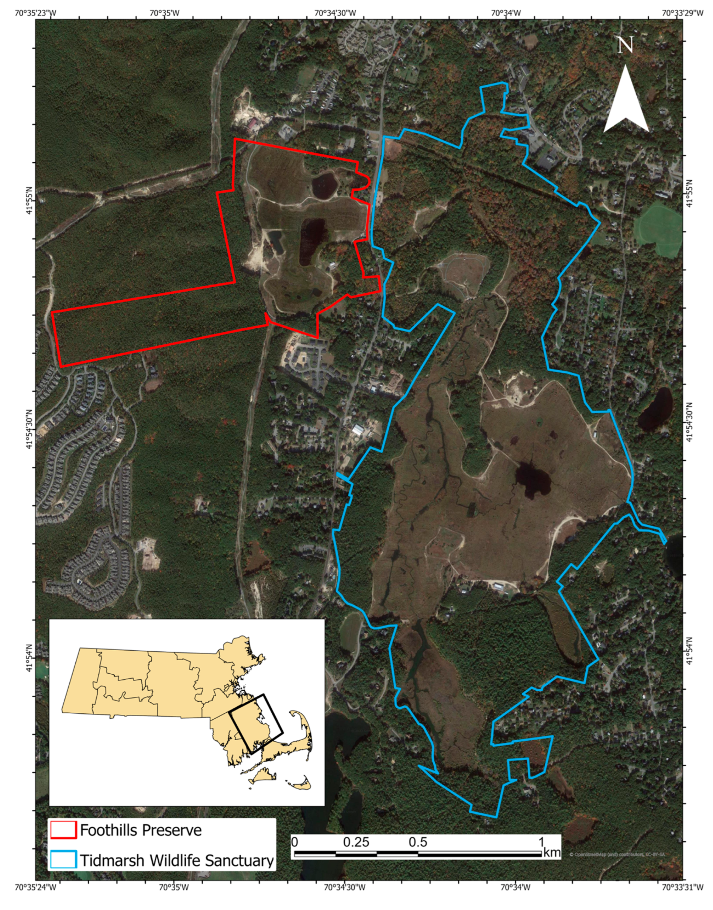
2.1. Study Sites

We centered this study on former commercial-scale cranberry farms in Southeastern Massachusetts (MA), USA, that were withdrawn from production and subsequently restored into wetlands (Figure 1). The American cranberry (Vaccinium macrocarpon), an evergreen perennial dwarf shrub with a trailing-vine habit, thrives in North American temperate wetlands [32]. With the international cranberry market becoming more competitive and the adoption of cost-effective, innovative farming methods elsewhere, cranberry farms in MA, especially those cultivated for centuries, are increasingly being retired and taken out of production [33,34]. The retirement of farmed bogs in Massachusetts can be attributed to the rising production costs, declining cranberry prices, the environmental impacts of cranberry farming, and the influences of climate change [34,35]. These circumstances created opportunities to restore these retired cranberry farms into natural wetlands [30,36].

Our research focused on two study sites (Figure 1) that underwent restoration at different timeframes: the Mass Audubon Tidmarsh Wildlife Sanctuary (5 YSR) and the Foothills Preserve (1 YSR), both situated in Plymouth, MA. Originally, both the Tidmarsh Wildlife Sanctuary and the Foothills Preserve were concurrently managed for commercial cranberry production [37]. These cranberry bogs featured multiple, alternating layers of sand and peat, with irrigation channels surrounding low-lying fields of cranberry crops [38]. Initiated in 2010 with the cessation of farming, the restoration interventions were successfully concluded in 2016 at the 5-YSR site. The farming operations in the neighboring site, the Foothills Preserve, ceased production in 2017, and restoration was completed in early 2021 [31]. Restoration efforts at both sites involved extensive landscape modifications, including the creation of various new habitat types [30,31,39]. Both the 1 and 5-YSR sites experienced similar restoration actions. Key actions comprised the removal of dams and other water-control structures to establish the longitudinal connectivity of the flow-through stream networks. Ponds and off-channel depressions were constructed to hold water year-round, enhancing natural wetland functions. Large woody debris was strategically scattered, and a significant number of native wetland trees, shrubs, and herbaceous plants were introduced, along with Atlantic white cedar plants (Chamaecyparis thyoides (L.) Britton, Sterns, and Poggenb). The 5-YSR site now encompasses over 481 acres of streams, ponds, forests, woodlands, and wetlands. In contrast, the 1-YSR site, with a total area of about 128 acres, including 50 acres previously devoted to cranberry bogs, is at an earlier stage in its recovery process.

2.2. Field Surveys

We conducted our survey from mid-May to early August 2022, utilizing two standard techniques to survey various habitat types at both the 1-YSR and 5-YSR sites, including open waters, marshes, and streams: (1) deploying and overnight recovery of non-lethal standard baited aquatic traps and (2) conducting active and visual encounter surveys in designated plots. Both methods are widely accepted by the scientific community and have been successfully employed in similar studies [40,41,42,43]. The aquatic traps targeted adult herpetofauna, while the plots focused on larval amphibians. Sampling was carried out between May and August, with three consecutive trap nights and one plot survey day per week, while opportunistically documenting visual and auditory encounters. Sampling activities between the 1- and 5-YSR sites were conducted concurrently. The sampling period coincided with the growing season, during which the herpetofauna activity was at its peak. For each trap and plot, we recorded the species identity and relative abundance of each species captured. Following proper identification, all captured animals were released back to their capture site.

For aquatic trapping, we employed funnel traps (Promar collapsible live bait trap, dimensions 92 × 30 × 30 cm, Prolomar and Ahi USA, Gardena, CA, USA) baited with oil-immersed sardines, and the bait was replenished in successive deployments. When selecting trap deployment sites, water depth, flow, and the surrounding natural structures were taken into consideration to ensure strategic placements for successful captures. Plots (10 × 10 m) were set up in marshes where aquatic traps were impractical. Within each plot, we estimated and recorded the surface water cover, actively searching under natural cover and substrates. We utilized dip nets to capture animals in standing water, with 1–2 sweeps for smaller and shallower areas and 2–3 sweeps for larger and deeper areas. Plot surveys were conducted weekly, where each plot was surveyed by two trained field personnel actively searching for an average of 30 minutes. Before dip-netting, we visually scanned the plot and lifted and searched through the natural cover. Additional visual or auditory encounters were opportunistically recorded but were not included in the statistical analyses, contributing solely to our species inventory.

Each of the 1-YSR and 5-YSR sites encompassed four habitat types, including large ponds (>14,000 m²), small ponds (<14,000 m²), streams, and marshes. For each habitat type, we designated trapping and plot locations, with an average replication of each habitat type four times per site. At the 1-YSR site, three large pond locations featured a minimum of three traps deployed per location, while four small pond locations and five stream locations had a minimum of two traps deployed per location. Additionally, two marsh locations with adequate surface water and depth had a minimum of two traps deployed. For plots at the 1-YSR site, nine marsh locations were designated, each with one plot. At the 5-YSR site, two large pond locations featured a minimum of three traps deployed per location, while four small pond locations and three stream locations had a minimum of two traps deployed per location. Two marsh locations with sufficient surface water and depth had a minimum of two traps deployed. For plots at the 5-YSR site, five marsh locations were designated, each with one plot. The number of traps and plots per site was contingent on the spatial extents and arrangements, ensuring spatial independence through a Moran’s I test based on georeferenced coordinates.

2.3. Statistical Analyses

2.3.1. Compare Species Richness and Abundance Through Univariate Tests

Given that the response variables (relative abundance and species richness) deviated from a Gaussian distribution and exhibited high levels of heteroscedasticity and that our sampling efforts were unevenly distributed between the 1-YSR and 5-YSR sites, we chose robust tests for our univariate statistical analyses for both the trap and plot surveys. Robust statistical methods demonstrate lower sensitivity to deviations from normality while maintaining reasonable and reliable performance [44,45]. Resistant to the influence of outliers and heavy-tailed distributions, robust statistical models remain asymptotically unbiased against variable sample sizes, offering computationally efficient and rigorous alternatives to classical and non-parametric statistics [46,47]. To address dissimilar trapping efforts among various sampling locations, we calculated catch per unit effort as the number of individuals or species captured per trap night per deployment site to standardize the trap data across different sampling locations (Equations (1) and (2)). All statistical analyses were conducted using the R (version 4.4.2) programming language for statistical computing and graphics [48] within the RStudio (version 2024.09.1) integrated development environment [49].

Species richness = (Total number of species captured per trapping site per night)/(Number of traps deployed at the site)

(1)

Relative abundance = (Total number of individuals captured for a given species per trapping site per
night)/(Number of traps deployed at the site)

(2)

As both our plot dimensions and survey efforts remained consistent across all plots, we did not standardize the plot data. To address the potential temporal effects on captures and control for the sampling date as a covariate, we employed a repeated-measure approach in all univariate analyses.

To assess differences between the 1-YSR and 5-YSR sites in terms of the herpetofaunal species richness and total abundance, we conducted a robust heteroscedastic analysis of variance (robust ANOVA) using trimmed means, where either species richness or relative abundance was the response variable. Meanwhile, the time since restoration (one vs. five years) was the predictor variable. This test, implemented with the R package (version 1.1-6) WRS2 [50], is not dependent upon the assumption of homoscedasticity, making it tolerant of unequal variances between groups [50]. It computes F-distributed Welch-type test statistics on trimmed means, where the most extreme values are replaced by neighboring values [50]. Additionally, we investigated whether herpetofaunal species richness and abundance varied significantly among different habitats at the 1-YSR and 5-YSR sites for the trap data using Yune’s trimmed means test. To correct the probabilities for multiple pairwise comparisons and decrease the false discovery rate, we applied the Benjamini–Hochberg procedure (R package: statsExpressions, version 1.1-6 [51]). We conducted robust ANOVA and pairwise comparison tests on all herpetofauna collectively and separately for amphibians and reptiles.

2.3.2. Explore Variations in Community Composition Through Multivariate Ordinations

To explore the associations between herpetofaunal community composition and the time since restoration (1-YSR and 5-YSR), we conducted non-metric multidimensional scaling (NMDS) for both the trap and plot data. For the trap data, we also examined community composition concerning different habitat types at 1- and 5-YSR, while for the plot data, we explored the association with different extents of surface water cover at the plot scale. NMDS is a powerful and robust approach to graphically summarize complex and highly dimensional community-scale data into a tractable number of dimensions, revealing disparities among biological communities [52,53,54]. Its computational rigor, tolerance for imbalanced sampling designs, outliers, and moderate background noise make it widely used in ecological community analyses [55,56,57,58,59].

For NMDS execution, we calculated the community dissimilarities for the plot and trap data, converting them into Bray–Curtis distance matrices [60] between the survey locations (R package: vegan, function: metaMDS, 2.6-10 [61]). The distance matrices underwent square-root transformation and Wisconsin double standardization [62]. To minimize stress, we employed monotone regression and treated ties by allowing equal observed dissimilarities to have different fitted values. Linear regression was applied if dissimilarities fell below 0.8 [63,64]. Stress calculations involved assigning zero as ordination distances under the null model [63,64]. After constructing an initial configuration with a minimum of 100 and a maximum of 1000 random starts, we ran 1000 iterative adjustments until a stable solution was reached with the lowest possible stress levels. Standardizing the NMDS results involved centering and scaling the final scores to unit root mean squares, rotating standardized scores to principal components, computing expanded weighted average species scores, and adding those to the site ordination. To diagnose the goodness of fit of the final NMDS solution, we created a scatterplot of the interpoint distances in the ordination plot against the original dissimilarities (Shepard plot) and plotted the stress values against the increasing dimensionality (scree plot). To test the significance of the NMDS solution, we evaluated if the NMDS is extracting stronger dimensions than expected by chance via running a randomization test based on a Monte Carlo simulation with 20 iterations of the community matrices and subsequently compared the stress obtained from randomized community data against the actual dataset.

Following NMDS, we implemented a permutational multivariate analysis of variance (PermMANOVA) to test the effects of time since restoration, habitat type, and surface water cover on community structure (R package: vegan, function: adonis [61]). PermMANOVA geometrically partitions variation in the distance matrices by permuting them to assess the significance of pseudo-F ratios [65]. Robust against dispersion effects, less sensitive to heterogeneity and correlation structures, distribution independent, and powerful in detecting community structure changes, PermMANOVA accommodates unbalanced asymmetrical designs, nested structures, and repeated measures [65,66]. To perform a PermMANOVA, we generated Bray–Curtis distance matrices [60] to quantify the compositional dissimilarity among the communities between different survey locations. We included the square root of the dissimilarities into the PermMANOVA model to elucidate the dissimilarities, which were added as a constant to the non-diagonal dissimilarities to avoid negative eigenvalues [67]. We used the relative abundance of herpetofauna to construct distance matrices, performed 1000 permutations, and included the main effects of habitat type, years since restoration, and their interaction as predictors. We defined the date of the survey as the repeated measure and identified specific survey locations as the nested covariates within both habitat types and years since restoration. This procedure was applied to both the trap and plot data. Given that the plot data shared the same habitat type, the percent surface water coverage replaced habitat type as a predictor.

To visualize compositional similarities, we conducted an analysis of the multivariate homogeneity of group dispersions (R package: vegan, function: betadisper; [68]). Testing for significant group dispersion differences among the years since restoration and habitat types, we visually represented the among-group versus within-group differences in community dissimilarities. Euclidean distances between group members and the group centroid were calculated based on principal coordinate axes. Next, to test if the group dispersions for years since restoration and among habitat types are significantly different, the distances of the group members to the group centroid were subject to a permutation test with 1000 iterations. Finally, to graphically visualize the among-group versus within-group differences in the community dissimilarities, we extracted the two principal coordinates that collectively account for the highest dispersion and ordinated the group centroids and principal ordinate scores for original Bray–Curtis community dissimilarities in the multivariate space.

2.3.3. Explore Species-Specific Responses Through Indicator Species Analyses

We employed indicator species analyses (ISA) to identify individual species or assemblages uniquely associated with the time since restoration. ISA indices, derived from relative abundance and occurrence, provided insights into the strength of species associations with different habitats [69], where the statistical significance of these associations was determined through randomization techniques [27,56]. The ISA values increase as a species exhibits a higher relative abundance and frequency in a particular habitat or community [54]. The ISA process began with a multi-level pattern analysis using the point biserial correlation coefficient with corrections for unequal sampling efforts among sites [70] as the species-site group association function. The analysis generated multiple combinations of input clusters (i.e., years since restoration), comparing each combination with the species in the community matrix (R package: indicspecies, function: multipatt, version 1.7.15). For each species, the analysis selected the combination with the highest association value, and the best matching patterns were tested for statistical significance, resulting in a species list strongly associated with the 1-YSR and 5-YSR sites. Next, we explored whether certain herpetofauna species combinations are consistently and specifically associated with either the 1-YSR or 5-YSR sites. Using the herpetofaunal survey-generated species abundance data, we created a matrix with all possible species combinations, where each row represented a survey location, and each column represented a species (package: indicspecies, function: combospecies). Constrained by a minimum and maximum number of species in combinations one and three, respectively, we performed a multi-level pattern analysis on the species combinations matrix to identify indicator species combinations that are specifically indicative of the 1-YSR or 5-YSR sites. All randomization tests in the indicator species analyses involved 1000 permutations.

3. Results

3.1. Overview

When all survey methods were combined, we identified nine amphibian and three reptile species at the 1-YSR sites, and nine amphibian and five reptile species at the 5-YSR sites (

Table 1. The presence or absence of all documented amphibian and reptile species in the one year since restoration site (1-YSR) and the five years since restoration site (5-YSR), as well as different habitat types nested therein. Presence or absence was determined using both trapping and plot data, as well as opportunistic observations, combined. The years since restoration column indicates where each species was found: 1-YSR site only (1), 5-YSR site only (5), or both (B). The life-history stage column states what life-history stages were found for each species: adult (A), larval (L), or egg masses (E). An ‘x’ indicates the presence of a species in a given habitat type.

Scientific Name	Vernacular Name	Years Since Restoration	Large Pond	Marsh	Small Pond	Stream	Life-History Stage
Amphibians
Ambystoma maculatum	Spotted salamander	B		x			E, L
Anaxyrus americanus	American toad	B	x	x			E, L, A
Anaxyrus fowleri	Fowler’s toad	B				x	E, L, A
Dryophytes versicolor	Gray tree frog	B		x			L
Lithobates catesbeianus	American Bullfrog	B	x	x	x	x	L, A
Lithobates clamitans	Green Frog	B	x	x	x	x	L, A
Lithobates palustris	Pickerel frog	B		x			L, A
Lithobates sylvaticus	Wood frog	B		x			E, L, A
Pseudacris crucifer	Spring peeper	B		x			E, L, A
Reptiles
Chelydra serpentina	Common snapping turtle	B	x		x	x	A
Chrysemys picta	Eastern painted turtle	B	x	x	x	x	A
Sternotherus odoratus	Eastern musk turtle	5	x		x		A
Thamnophis sauritus	Eastern ribbon snake	5		x			A
Thamnophis sirtalis	Common garter snake	B		x			A

). Both the 5-YSR and 1-YSR sites shared 12 species in common, including the American bullfrog (Lithobates catesbeianus (Shaw, 1802)), American toad (Anaxyrus americanus (Holbrook, 1836)), common snapping turtle (Chelydra serpentina (Linnaeus, 1758)), eastern painted turtle (Chrysemys picta (Schneider, 1783)), Fowler’s toad (Anaxyrus fowleri (Hinckley, 1882)), common garter snake (Thamnophis sirtalis (Linnaeus, 1758)), gray tree frog (Dryophytes versicolor (LeConte, 1825)), green frog (Lithobates clamitans (Latreille, 1801)), Pickerel frog (Lithobates palustris (LeConte, 1825)), spotted salamander (Ambystoma maculatum (Shaw, 1802)), spring peeper (Pseudacris crucifer (Wied-Neuwied, 1838)), and wood frog (Boreorana sylvaticus (LeConte, 1825)) (Table 1). Species exclusive to the 5-YSR included the eastern musk turtle (Sternotherus odoratus (Latreille in Sonnini and Latreille, 1801)) and the eastern ribbon snake (Thamnophis sauritus (Linnaeus, 1766)). Spotted salamanders were the most abundant larval amphibian at both the 1- and 5-YSR sites, followed by spring peepers and wood frogs, which occurred at similar frequencies. Eastern painted turtles were the most abundant reptile, while American bullfrogs were the most frequently captured adult amphibian at both restoration time points.

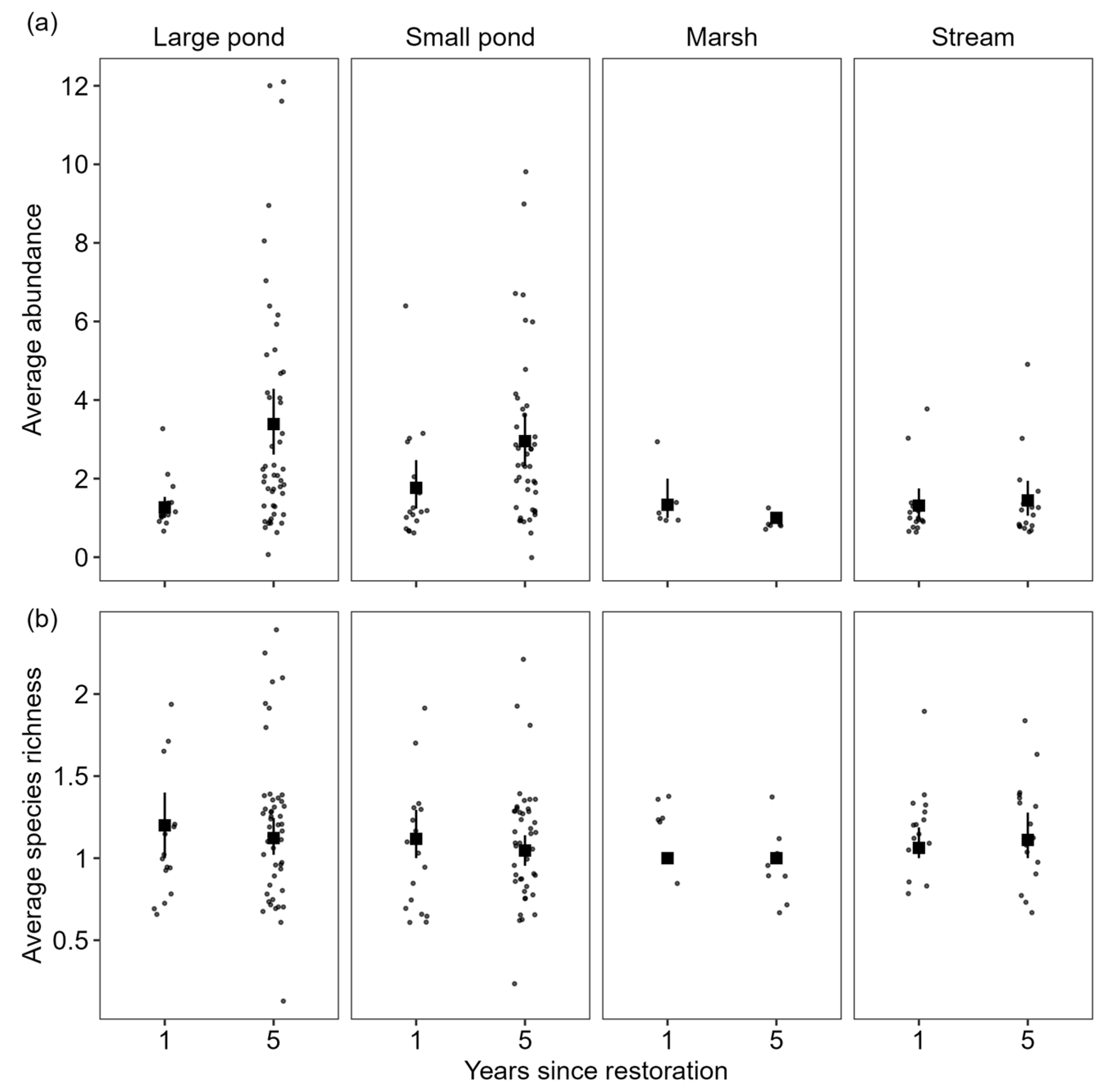
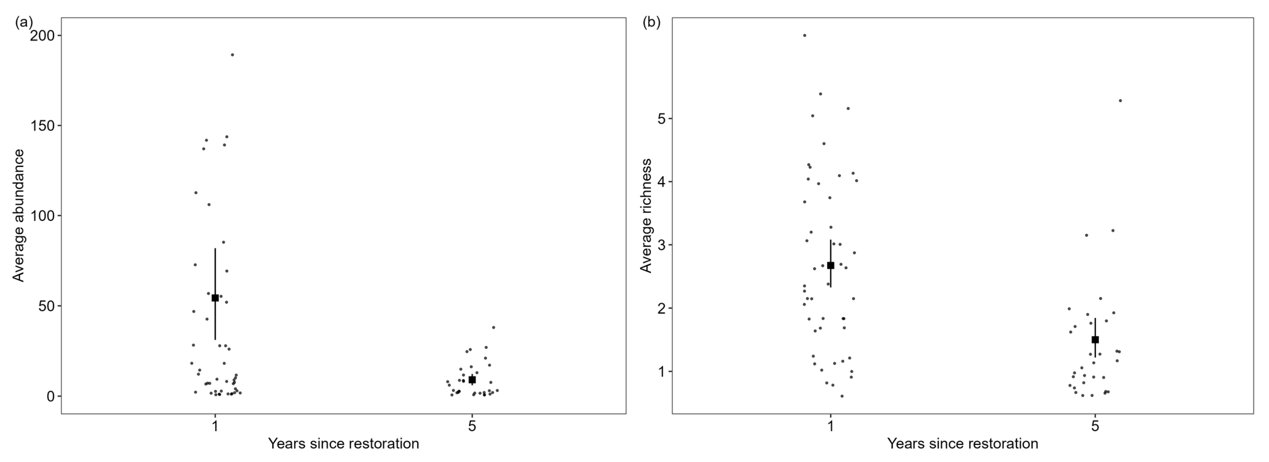
3.2. Variation in Species Richness and Abundance Among Herpetofauna in Response to Restoration

Adult amphibian richness and abundance were significantly greater at the 1-YSR sites than at the 5-YSR sites (robust ANOVA: F = 0.47, p < 0.0001). In contrast, adult reptiles showed opposing trends, with the 5-YSR sites surpassing the 1-YSR sites in both richness (robust ANOVA: F = 0.38, p ~ 0.001) and abundance (robust ANOVA: F = 1.34, p < 0.0001). When adult amphibians and reptiles were taken together, the average herpetofaunal species richness did not differ significantly between 1 YSR and 5 YSR (robust ANOVA: F = 0.01, p > 0.05), despite a higher average number of species at the 5-YSR sites. In contrast, the total herpetofaunal abundance significantly differed between the 1-YSR and 5-YSR sites (robust ANOVA: F = 1.29, p < 0.0001), where both the average abundance and variability were greater at the 5-YSR sites compared to the 1-YSR sites. The larval amphibian species richness (robust ANOVA: F = 1.17, p < 0.0001), as well as the abundance (abundance-robust ANOVA: F = 45.3, p < 0.01) exhibited significant differences between sites in response to time since restoration with both metrics being greater at the 1-YSR sites.

Follow-up pairwise comparisons between habitats indicated significant differences in adult herpetofaunal abundance between large ponds and marshes (t = 1.65, p < 0.001), large ponds and streams (t = 1.14, p < 0.0001), marshes and small ponds (t = 1.39, p < 0.001), and small ponds and streams (t = 1.15, p < 0.001) (Figure 2). Significant differences in adult herpetofaunal richness were observed only between large ponds and marshes (t = 0.15, p < 0.05) (Figure 2). Disparities in adult species richness between the 1-YSR and 5-YSR sites were primarily driven by differences in richness at lentic habitats. Adult amphibian richness exhibited pronounced significant differences among different habitat types between large ponds and marshes (t = −0.89, p < 0.0001), large ponds and streams (t = −0.21, p < 0.05), marshes and small ponds (t = 0.91, p < 0.0001), marshes and streams (t = 0.68, p < 0.0001), and small ponds and streams (t = −0.24, p < 0.05). Likewise, adult amphibian abundance displayed notable significant differences among different habitat types between large ponds and marshes (t = −1.03, p < 0.0001), large ponds and streams (t = −0.24, p < 0.05), marshes and small ponds (t = 1.04, p < 0.0001), marshes and streams (t = 0.79, p < 0.0001), and small ponds and streams (t = −0.25, p < 0.05) (Figure 2). Pronounced significant differences in reptile richness among different habitat types were evident between large ponds and marshes (t = 1.02, p < 0.0001), marshes and small ponds (t = −0.97, p < 0.0001), and marshes and streams (t = −0.76, p < 0.0001), whereas the significant differences in reptile abundance among different habitat types were evident between large ponds and marshes (t = 2.66, p < 0.0001), large ponds and streams (t = 1.63, p < 0.0001), marshes and small ponds (t = −2.38, p < 0.0001), marshes and streams (t = −1.03, p < 0.0001), and small ponds and streams (t = 1.35, p < 0.0001). Both larval amphibian abundance and richness at the 1-YSR site exhibited substantial variations between plots (Figure 3), indicating high spatial heterogeneity in larval occupancy. The plots with stable and prolonged hydroperiods recorded the highest amphibian larval abundance, as well as species richness.

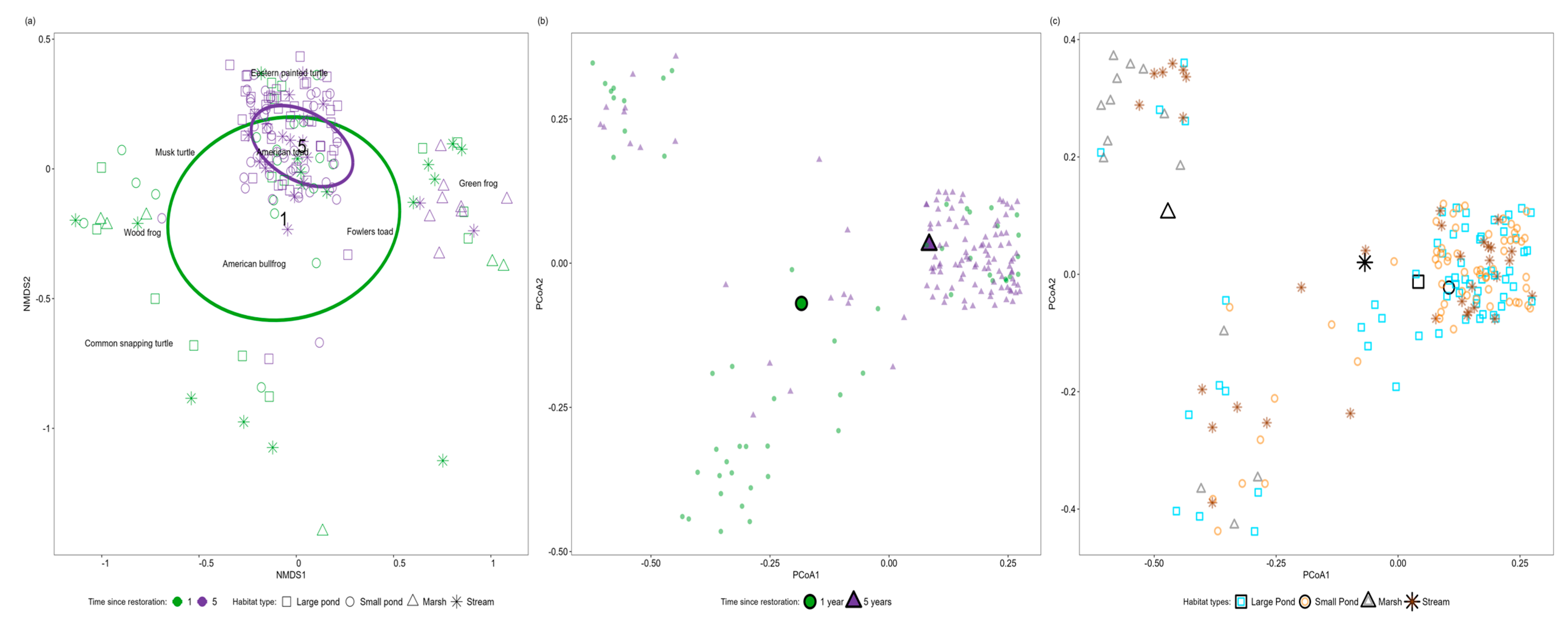
3.3. Variations in Community Composition in Response to Restoration

The NMDS analyses for adult herpetofauna and larval amphibians converged after 110 and 198 iterations (starting from a random configuration), respectively. Shepard plots showed strong correlations between the observed and ordinated dissimilarities for both linear (adult herpetofauna R² = 0.96; larval amphibians R² = 0.93) and non-metric (adult herpetofauna R² = 0.99; larval amphibians R² = 0.98) fits. The narrow scatter around the line of best fit and low-stress values (adult herpetofauna: 0.02; larval amphibians: 0.01) indicated an ‘excellent’ fit. The scree plot supported stress reduction with lower dimensionality, retaining maximized interpretative capability. Monte Carlo randomization tests showed that our NMDS solution extracted stronger dimensions than expected by chance, confirming the non-random community organization (adult herpetofauna: mean stress = 0.3, standard deviation = 0.002; larval amphibians: mean stress = 0.51, standard deviation = 0.004; actual NMDS solution = 0.02).

The two-dimensional NMDS ordination plots revealed substantial dissimilarities in adult herpetofaunal communities between the 1-YSR and 5-YSR sites, while the 1-YSR sites displayed greater variation in the community composition than the 5-YSR sites (Figure 4). Although the 5-YSR covariance ellipse fell mostly within that of 1-YSR, the centroids ordinated separately, indicating non-trivial community composition differences. The ordination plot illustrated varied herpetofaunal responses to both time since restoration and habitat type. Eastern painted turtles and musk turtles were primarily associated with 5-YSR, preferring streams and large or small ponds, respectively, while common snapping turtles were more frequent in the 1-YSR across habitats. American bullfrogs and green frogs exhibited broad habitat associations but were mainly found in the 1-YSR. Wood frogs were associated with the 5-YSR, whereas American and Fowler’s toads favored the 1-YSR without habitat differentiation.

The NMDS ordination showed minimal differences in larval amphibian communities between the 1-YSR and 5-YSR sites, with no clear associations with surface water coverage. Neither factor significantly influenced community composition or habitat associations, indicating weak responsiveness of larval amphibians to restoration time and surface water extent. The covariance ellipses for the 1-YSR and 5-YSR sites largely overlapped, and their centroids ordinated closely, indicating minimal separation in ordination space. Distinguishable habitat association patterns were limited to a handful of species. Spotted salamanders were primarily associated with the 5-YSR sites and showed a stronger preference for lower (0–50%) surface water coverage, regardless of restoration age. Three species were more closely associated with the 5-YSR sites, while five species showed stronger associations with the 1-YSR sites. Most species (gray tree frog, spring peeper, wood frog, Pickerel frog, green frog, and American toad) showed slightly stronger affinity for greater (51–100%) surface water cover.

The PermMANOVA analysis indicated that habitat type (F = 17.030, p < 0.0001), time since restoration (F = 28.60, p < 0.0001), and their interaction (F = 4.930, p < 0.0001) significantly influenced the community composition of adult herpetofaunal community composition. Habitat type explained nearly a fifth (SS = 4.47, R² = 0.20) of the community dissimilarity, while time differences since restoration accounted for a tenth (SS = 2.50, R² = 0.11). The interaction between these variables contributed to 6% (SS = 1.20, R² = 0.06) of the community dissimilarity. This suggests that, for a given time since restoration, community composition varied across different habitat types. While time post-restoration significantly influences adult herpetofaunal community structure, the distinction between the 1- and 5-YSR sites remains weak, as indicated by low effect sizes. In contrast, the PermMANOVA showed that the effects of surface water coverage (F = 0.70, R² = 0.01; p > 0.05) and time since restoration (F = 1.89, R² = 0.024; p > 0.05), as well as their interactions (F = 0.36, R² = 0.004; p > 0.05), were not significant drivers of the larval amphibian community composition. This suggests that the community dissimilarity observed among larval amphibians across survey sites is not driven by differences in surface water coverage, time since restoration, or their interaction.

The principal coordinate (PCoA) plots based on the analysis of multivariate homogeneity of group dispersions revealed notable distinctions in adult herpetofaunal community organization in response to years since restoration, particularly concerning group centroids (Figure 5). The community dissimilarity between marshes and other habitat types was most pronounced, as indicated by the distance between their corresponding centroids. Although centroids for large and small ponds, as well as streams, were separated, the community dissimilarities between these habitats were less pronounced, as reflected by the close distance between their corresponding centroids. The principal coordinates used for the ordination plot explained >80% of the adult herpetofaunal community dissimilarity. The test for the multivariate homogeneity of group dispersions demonstrated significantly greater among-group dispersion than within-group dispersion (ss = 2.57, F = 98.66, p < 0.0001), indicating much greater community dissimilarity between the 1-YSR and 5-YSR sites than within either the 1-YSR or 5-YSR sites. Among-group dispersion was also significantly greater than within-group dispersion concerning habitat types (ss = 3.00, F = 937.97, p < 0.001), further confirming the influence of different habitat types arising from restoration as a determinant of herpetofaunal community structure.

In contrast, the PCoA plots for larval amphibians showed a less distinct community organization in response to both years since restoration and surface water coverage. (Figure 5). The community dissimilarity between the 1-YSR and 5-YSR sites, as well as between 0–50% and 51–100% surface water coverage, was minimal, as reflected by the close ordination distance between the corresponding centroids. The principal coordinates used for the ordination plot explained 86% of larval amphibian community dissimilarity. The test for homogeneity of multivariate dispersion also revealed non-significant distinctions in both among-group dispersion and within-group dispersion (ss = 0.005, F = 0.97, p > 0.05), indicating minimal community dissimilarity between the 1-YSR and 5-YSR sites. The among-group dispersion similarly showed non-significant distinctions within groups concerning surface water cover (ss = 0.002, F = 0.51, p > 0.05).

3.4. Species-Specific Responses to Restoration

The multilevel pattern analysis also indicated species-specific habitat associations influencing the community composition of adult herpetofauna at the 1-YSR vs 5-YSR sites (

Table 2. Multilevel pattern analysis displaying species associations of adult herpetofauna with one year since restoration (1-YSR) and five years since (5-YSR) restoration sites. Reported from adult herpetofauna recorded in trap surveys at sites (Tidmarsh Wildlife Sanctuary and Foothills Preserve, Plymouth, MA, USA). An ‘x’ indicates the presence of a certain species.

Species	1-YSR	5-YSR	Test Statistics	p-Value
American bullfrog	x		0.336	0.000 ***
American toad	x		0.097	0.307
Common snapping turtle	x		0.284	0.000 ***
Fowler’s toad	x		0.097	0.000 ***
Green frog	x		0.161	0.061
Wood frog	x		0.097	0.307
Eastern painted turtle		x	0.506	0.000 ***
Musk turtle		x	0.170	0.014 *

(Significant differences: p ≤ 0.001: ***; p ≤ 0.01: *.

). The American bullfrog, common snapping turtle, and Fowler’s toad demonstrated statistically significant associations with the 1-YSR sites, whereas the eastern painted turtle and the musk turtle exhibited significant associations with the 5-YSR sites. The remaining species showed no distinct association between sites with different time frames since restoration. Furthermore, while multiple herpetofaunal species exhibited associations with the 5-YSR vs 1-YSR sites, individual species appeared to serve as more effective indicators of the 5-YSR vs 1-YSR sites than species combinations. Notably, the American bullfrog (test statistics = 0.34, p < 0.05), common snapping turtle (test statistics = 0.28, p < 0.05), Fowler’s toad (test statistics = 0.097, p < 0.05), and eastern painted turtle (test statistic = 0.51, p < 0.05) were identified as significant indicators of 1-YSR sites. However, individual species, as well as species combinations, were notable indicators of 5-YSR sites (eastern painted turtle: test statistics = 0.51, p < 0.001; musk turtle and eastern painted turtle: test statistic = 0.17, p < 0.05).

In contrast, the multilevel pattern analysis for larval amphibians revealed statistically insignificant associations of species between the 1-YSR vs 5-YSR sites, except for two species with weak, statistically significant associations with the 1-YSR site. The American bullfrog (test statistic = 0.206, p < 0.05) and spotted salamander (test statistic = 0.221, p = 0.05) exhibited marginally significant associations with the 1-YSR sites. The remaining species showed no distinct association between the sites with different time frames since restoration (

Table 3. Multilevel pattern analysis displaying species associations among larval amphibians with one year since restoration (1-YSR) and five years since (5-YSR) restoration sites. Reported from larval herpetofauna recorded in plot surveys at sites (Tidmarsh Wildlife Sanctuary and Foothills Preserve, Plymouth, MA, USA). The American bullfrog and spotted salamander showed statistically significant associations with 1-YSR sites. An ‘x’ indicates the presence of a certain species.

Species	1-YSR	5-YSR	Test Statistics	p-Value
American bullfrog	x		0.206	0.028 *
Green frog	x		0.023	0.844
Spotted salamander	x		0.221	0.050
Spring peeper	x		0.004	0.974
Toad	x		0.018	0.867
Wood frog	x		0.016	0.892
Gray tree frog		x	0.206	0.071
Pickerel frog		x	0.138	0.280

(Significant differences: p ≤ 0.01: *).

). Combinations of larval amphibians, involving the American bullfrog (American bullfrog + spring peeper: test statistic = 0.25, p < 0.05) or spotted salamander (spotted salamander + wood frog: test statistic = 0.27, p < 0.05) appeared to be more indicative of 1-YSR sites. Conversely, the combination of the green frog, Pickerel frog, and wood frog emerged as a strong indicator for the 5-YSR sites (test statistic = 0.13, p < 0.05). Furthermore, multiple larval amphibian species displayed associations with both the low (0–50%) and high (51–100%) surface-water coverage. The combination of green frog, Pickerel frog, and wood frog seemed to be the most reliable indicator for the low (0–50%) surface-water coverage (test statistics = 0.126, p < 0.05). Additionally, the American bullfrog (test statistics = 0.206, p < 0.05) and various species combined with the American bullfrog appeared to be strong indicators for the 51–100 surface water coverage range (American bullfrog and spring peeper: test statistics = 0.246, p < 0.05; American bullfrog and spotted salamander: test statistics = 0.186, p < 0.05; American bullfrog and spotted salamander and spring peeper: test statistics = 0.243, p < 0.05).

4. Discussion

Our research into herpetofaunal communities in restored wetlands has unveiled intricate and contrasting responses from amphibians and reptiles to time since restoration. We observed nuanced patterns in community composition, total abundance, and richness between sites at varying post-restoration stages. Noteworthy distinctions emerged between adult and larval amphibians, as well as reptiles, highlighting the multifaceted, complex, and incongruent responses by distinct taxa to restoration efforts. We substantiated the influence of time since restoration on herpetofaunal communities, reaffirming the dynamic nature of post-restoration ecological trajectories. Specifically, we found that as restoration age increased, reptile richness and abundance increased while the same diversity metrics for amphibians decreased. Restoration age significantly influenced adult herpetofaunal community structure, particularly in relation to habitat types created through restoration. However, neither factor had a discernible impact on larval amphibian community composition. Our findings indicated the presence of both amphibians and reptiles in all restored wetlands, regardless of their restoration age. Despite well-documented temporal changes in abundance, biomass, taxonomic richness, dominance ranks, and species turnover at community or assemblage scales in both terrestrial [71,72] and aquatic realms [73,74,75], there is a paucity of similar studies on wetland restoration with a herpetofaunal perspective. Existing research on amphibian occupancy in restored wetlands primarily revolves around comparisons between restored and reference wetlands [76,77,78]. Our study addresses this gap by comparing sites at different stages post-restoration, thus offering a more nuanced understanding of herpetofaunal responses to restoration efforts. Additionally, our study employs statistical rigor and a systematic, reproducible design, ensuring scientifically robust inferences that can effectively inform restoration actions.

Although reptilian richness and abundance exhibited a positive response to restoration age, as we initially hypothesized, unexpected disparities emerged in adult and larval amphibian diversity between the 1-YSR and 5-YSR sites. Both amphibian richness and abundance decreased with time since restoration, with larvae showing a stronger response than adults, highlighting the importance of considering life-history stages. While restoration age and habitat types significantly influenced adult herpetofaunal community composition, this was not the case for larval amphibians, suggesting that adult community turnover is more strongly shaped by these factors, while larval communities show limited turnover across sites with different restoration ages or habitat types.

The amphibian responses we evidenced challenge the long-held consensus that prolonged post-restoration trajectories lead to greater abundance and diversity [79,80,81]. Amphibians often exhibit limited dispersal abilities, breeding-site fidelity, and philopatry, which may restrict their ability to access and colonize recently restored wetlands [82,83,84]. Despite these challenges, 1-YSR sites showed greater amphibian colonization. The observed differences in amphibian richness, abundance, and larval community composition between the restoration trajectories are likely influenced by local drivers such as wetland depth and size, vegetation structure and biomass, substrate composition, hydroperiod, hydrochemical (pH, mineralization, oxygen content), and microclimatic stability, and predator density [85,86,87,88]. Wetlands within both the 1-YSR and 5-YSR sites inherently differed in local attributes [39], with the 1-YSR sites displaying early successional characteristics such as high surface water cover and low predation pressure, thus are conducive to larval amphibian survival and growth [89,90]. In contrast, the 5-YSR sites, given longer restoration trajectories, exhibited prolific vegetation growth, heightened evapotranspiration, reduced wetland hydroperiod, and elevated predator recruitment [91]. Deeper, hydrologically stable depressions, functionally analogous to vernal pools and ideal for larval growth, were more abundant in the 1-YSR sites, potentially enabling amphibians to opportunistically exploit predator-limited reproductive niches [92]. Although both the 1-YSR and 5-YSR sites underwent similar restoration actions, the 5-YSR site experienced more extensive interventions and had a longer restoration period (1 year vs. 6 months) and larger spatial extent, which may influence community structure. Wetland naturalization upon restoration is a slow process, with the formation of refugia, microhabitats, and new habitat features occurring over decades to centuries [23,93,94,95,96]. Delayed community turnover of vegetation and diatoms in restored salt marshes and streams suggests that restored ecosystems may take considerable time to develop the desired biophysical properties, habitat heterogeneity, and biogeochemical processes [91,97,98,99]. Therefore, reduced amphibian richness and abundance in the 5-YSR sites is attributable to suboptimal, transitional physicochemical properties that have not yet reached targeted conditions in natural wetlands.

The total herpetofaunal richness of all restored wetlands, irrespective of their restoration age, remained below the richness of the regional species pool, which is consistent with prior studies [76,85,100].

Dispersal barriers, including surrounding residential and commercial development, impervious surfaces, and transportation infrastructure, coupled with limited connectivity to natural wetlands and ecologically incompatible river crossings, could have hindered colonization, particularly for species with low vagility or high physiological sensitivity [101,102,103,104]. Additionally, modified land cover may act as an environmental filter, shaping species composition in restored wetlands [21]. Most herpetofauna we recorded across all restored wetlands were niche generalists with wide environmental tolerances, broad distribution ranges, and abundant, stable regional populations. Conversely, rare, range-restricted, conservation-dependent species or niche specialists were absent regardless of the restoration age. Our findings align with the core-satellite species hypothesis [105] suggesting that abundant, wide-ranging ‘core species’ readily exploit vacant niches in restored wetlands, while ‘satellite species’ with narrow environmental tolerance and specific niche requirements are less likely to establish. In the industrial Northeastern US, where centuries of land-use transitions have diminished the regional species pool, opportunistic and disturbance-tolerant generalists dominate [22,106]. This might partly explain the lower-than-expected diversity in our study. While restored wetlands may not support high numbers of conservation-dependent species, the presence of regionally common and widespread species can still optimize ecosystem functions [107]. As predicted by the mass ratio hypothesis and the selection effect, a few abundant or high-performing species can maintain functional and structural integrity [108,109]. This represents a key milestone in the restoration trajectory, signifying revitalized ecological processes, even if the taxonomic diversity targets are not fully met [110].

Chronological community-wide changes to restored wetlands can be exceedingly slow, while post-restoration systems can move towards alternative states or pass through multiple transient states that markedly differ from desirable reference states [111,112,113]. Even multiple decades after restoration, biological (e.g., plant and animal assemblage characteristics) and biochemical (e.g., carbon storage) properties of restored wetlands can still remain far below those of intact reference wetlands [96,113]. Communities exposed to chronic and extreme stressors, such as century-long industrial agricultural operations, can transition into alternative stable states that persist long after stress removal [21]. The lack of significant relationships between larval amphibian community composition and restoration efforts, with regards to neither restoration age nor emergent habitat types, is perplexing, albeit remarkable. The contrasting community responses suggest that larval amphibian communities are primarily shaped by neutral ecological processes, driven by stochastic fluctuations in demographic rates, which is consistent with the unified neutral theory [114]. In contrast, adult herpetofaunal community organization is influenced by deterministic processes, including functional traits, community interactions, and environmental conditions. These dynamics align with Eltonian niche theory (species’ functional roles and trophic positions) and Grinnelian niche theory (species’ environmental requirements and ecological specializations) [115].

Similar to our findings, ecological surprises have been documented in other regions. In Central and Northern Minnesota, USA, the age of restored wetlands did not significantly influence amphibian species richness [76]. Breeding population sizes and juvenile recruitment of amphibians showed no discernible temporal trends in constructed wetlands in the Carolina Bays of the US Atlantic Coastal Plains [85]. In the mid-Atlantic coastal plains of the US, newer ponds exhibited greater amphibian species composition and diversity metrics [116]. Influenced by hydrology, productivity, and soil dynamics, wetland restoration can follow diverse, non-linear trajectories resulting in complex biological responses that vary in the rate, magnitude, and direction [97]. These processes can trigger multiple causal pathways and feedback loops, leading to transient, temporally dynamic biological shifts [104]. Unexpected amphibian responses to restoration age may stem from these complex and dynamic trajectories. Such ecological surprises are not exclusive to herpetofauna, for example, abandoned cranberry bogs undergoing passive naturalization, and restored salt marshes showed no directional shifts in vegetation composition, density, or structural diversity along restoration trajectories [91,97,117].

Agricultural legacies inherent to farmed cranberry bogs, such as channelized, flow-regulated stream systems, structurally simplified cultivated bogs, and species-depauperate biological communities, may persist after restoration [99,118,119]. As restoration progressed, biotic influences, such as vegetation composition, biomass, and cover, became more impactful than agricultural legacies [117,120]. Consequently, the 1-YSR sites might sustain stronger impacts from the agricultural past than the 5-YSR sites, where relatively advanced successional stages experience fewer legacy effects, likely contributing to the reduced reptile diversity in the 1-YSR sites. As plant and animal colonization progresses, the influence of agricultural histories on community composition will diminish [121,122]. Variations in restoration intensity, pre-restoration conditions (flow-through vs. non-flow-through systems), and the extent of historical modifications (such as stream impoundments, channel alterations, and wetland changes) can result in confounding biological responses, overriding the influence of restoration age and leading to contradictory outcomes [118,123].

While our study revealed a negative relationship between amphibian species richness and abundance over time since restoration, previous studies from various ecosystems suggested that amphibians may benefit from advanced restoration age due to vegetative succession and ecosystem stability [124]. In the savannah–wetland mosaics of the Central US, restored ephemeral wetlands exhibited increased species richness, breeding sites, and a relative abundance of species with increasing time since restoration [125]. Similarly, older wetlands in the tall-grass prairies of the Midwestern US experienced greater amphibian colonization rates compared to newly restored wetlands [126]. In contrast, rapid increases in amphibian colonization, occupancy, and breeding populations have been observed within short timeframes of restoration in Northern European and Midwestern US wetlands [79].

Our findings revealed a notable increase in reptile diversity and abundance over time since restoration, which is attributable to temporally mediated, slow processes such as reptile colonization and establishment [89,90]. The habitat template—defined by both spatial configuration and temporal heterogeneity of habitat characteristics, as well as seasonal variations in environmental conditions—can strongly shape the dynamics of biological communities [127]. Wetland restoration, within certain temporal constraints, can create or augment habitat templates [22], thus contributing to increased reptile richness and abundance over time. Augmented reptile diversity over time since restoration, coupled with the strong influence of both restoration age and habitat types over adult herpetofaunal community turnover, align with theoretical concepts in the habitat template concept [127], ecological successional models [128], and the species–time relationship [129]. Our results are consistent with the analogous trends observed in wetland restoration initiatives elsewhere. For instance, North American rivers have witnessed increased fish passage and heightened fish life-history diversity following the removal of flood-control structures [104]. Similarly, Baecher et al. [103] observed an increased occupancy of reptile species of conservation concern in restored tall-grass prairie wetlands seven years after restoration. Restored wetlands in Southern California exhibited gradual increments in plant cover, species richness, and abundance of both aquatic insects and avifauna across 10 years [130]. Restored wetlands and streams undergo a series of processes, including the development of complex food webs and substrate heterogeneity, likely contributing to increased reptilian diversity in 5-YSR sites [104]. Restoration targets such as open riparian canopy, increased aquatic habitat acreage, and enhanced habitat quality for reptiles. Moreover, increased stream sinuosity enhances hydrological connectivity between channels and floodplain wetlands, further boosting habitat and resource availability [103]. Additionally, restoration efforts promote groundwater discharge, providing thermal buffering for reptilian metabolism, reproduction, and growth, including creating thermal refugia for freshwater turtles [131,132]. The process-based restoration approach implemented at our study sites has yielded desirable ecosystem states over time [133], explaining the observed improvements in reptilian diversity metrics as the wetlands age. While our study region is known to have populations of the invasive red-eared slider turtle (Trachemys scripta elegans (Wied-Neuwied, 1839)) [134,135], we found that this species was consistently absent from the wetlands we surveyed, regardless of their restoration age. However, the red-eared slider was previously reported at the 5-YSR sites in the earlier stages of post-restoration, albeit at lower frequencies [136,137]. The absence of red-eared sliders in our surveys suggests their failure to persist despite initial colonization, regardless of the successional stage, indicating a positive outlook for native herpetofaunal assemblages.

Our findings suggest niche segregation among herpetofauna, where reptiles and amphibians exhibited variable affinities toward the 5-YSR and 1-YSR sites, reflecting divergent restoration trajectories driven by differences in vegetation structure, water quality, surface water cover, depth, soil properties, and other physicochemical factors [138]. For instance, regionally common freshwater turtle species with broad niche associations, like eastern painted turtles and musk turtles, displayed notable associations with the 5-YSR sites, which offer hydrologically stable, large ponds with dense vegetation growth and complex substrates, as well as essential habitats like hibernacula and refugia [134,139] that develop in later-stage restored wetlands. Notably, geographically widespread, regionally common, habitat generalist amphibians (e.g., American bullfrog, green frog, and spring peepers) exhibited associations with the 1-YSR sites, reflecting their preference for early successional wetlands. The 1-YSR sites exhibited pronounced variations in adult herpetofaunal community structure than the 5-YSR sites, indicating dynamic assembly processes during early recovery. Species occupancy fluctuates both spatially and temporally in response to seasonal resource spikes or optimal thermal conditions [140,141], which are influenced by groundwater discharge, lateral water movements, and channel flow [15,142]. Our results indicate that longer restoration trajectories are driving the reshaping of communities as habitat structures evolve. Restoring wetlands at different times enhances landscape-scale hydrologic and habitat heterogeneity, supporting herpetofaunal survival and reproductive success [103,143]. Thus, we advocate for staggered restoration efforts to create diverse successional stages, promoting habitat heterogeneity, resource availability, and biodiversity [143,144].

While the variability in reptile richness and abundance was the highest in the 5-YSR sites, amphibians exhibited the highest variability in the 1-YSR sites, reflecting a patchy herpetofaunal distribution, implying spatial heterogeneity in habitat quality and resource distribution, highlighting non-uniform wetlands use by herpetofauna across time and space. These complex habitat associations highlight the need to account for local-scale, habitat-specific factors in restoration planning to better support diverse herpetofaunal communities [144,145]. The dynamic ecological states in restored wetlands, where species abundance and composition vary across space, may enhance resilience to anthropogenic perturbations [110]. Restoration goals should indeed account for past, legacy, and current disturbances, as well as the consequent spatiotemporal variability in species composition [21,119]. Although hydrologic gradients were incorporated into both the 1-YSR and 5-YSR sites [131,132], their influence varies temporally, shaping different restoration trajectories. These gradients contribute spatial heterogeneity in resource levels, environmental conditions, and fitness consequences, leading to patchy species occupancy across restored wetlands. Similar spatial heterogeneity has been observed in other restoration contexts, such as the patchy distribution of Atlantic White Cedar seedlings around mature seed trees [146].

Time since restoration shapes biological communities, but species occupancy in restored wetlands is also influenced by landscape-scale factors such as source population distribution, habitat connectivity, and watershed-scale processes (e.g., nutrient loading, sediment input) [22,147,148]. Restoration trajectories further depend on site manipulation intensity, target outcomes, and restoration methods [149].

The 1-YSR and 5-YSR sites—with similar habitat types, flow-through systems, ecoregions, geological and geographical backdrop, and comparable agricultural histories—provide a natural experiment to isolate the effects of restoration age. Their proximity within the same watershed also suggests comparable source–sink dynamics and metapopulation interactions. Thus, the observed differences in herpetofaunal communities are less confounded by extraneous variables and can be objectively attributed to factors linked to restoration trajectory [87,88].

We highlighted the critical role of time since restoration in shaping community assembly patterns. Nonetheless, restored forested wetlands may require multiple decades to achieve the desired ecological status [150]. Temporal shifts in aquatic and wetland community structure are influenced by ecological, physical, and geographical drivers [73], but the time elapsed since restoration in our study sites may be insufficient for these drivers to synergistically shape herpetofaunal assemblages. Furthermore, the process-based restoration approach in our study system implies ongoing habitat restructuring and formation, encompassing vegetation succession and growth [149], modifications to biogeochemical functions [23,98], and hydrological shifts [21]. These processes generate spatiotemporal heterogeneity in restored wetlands, expand niche breadth, and promote species recruitment, but biodiversity outcomes remain temporally constrained [104]. Long-term monitoring is needed to assess how shifts in wetland hydrodynamics (e.g., surface water cover, water depth) and vegetation structure drive habitat and niche diversification, influencing herpetofaunal communities, life-history stages, and species abundance distributions [151,152]. Given the diverse range of body sizes and trophic positions of herpetofauna, long-term monitoring may capture slow-responding species, particularly small-bodied taxa and higher trophic-level predators, revealing pronounced community distinctions over time [73].

Future Directions and Recommendations

Future restoration of retired cranberry farms into interconnected, wetland complexes with variable hydrologic regimes should account for both the local (e.g., hydroperiod, wetland size) and landscape scale (e.g., regional wetland density) drivers [153] to support species-specific habitat needs to enhance biodiversity [77,79,154]. This approach facilitates adaptive habitat switching, enhances population persistence, and strengthens ecosystem resilience to anthropogenic and climate stressors [155]. Given that wetland-dependent herpetofauna often range beyond wetland boundaries [156] and transverse terrestrial environments to access seasonal resources, incorporating upland connectivity is essential [157,158]. As wetlands form the interphase between aquatic and terrestrial realms, we urge natural resource managers to integrate upland habitat management into wetland restoration efforts [100,103,153,155].

Integrating species-specific habitat management strategies can substantially enhance biodiversity conservation in restored wetland ecosystems. For example, maintaining optimal amphibian breeding sites in ephemeral wetlands, along with providing secure nesting areas, can boost recruitment and overall population resilience [158]. Additionally, reducing trophic pressure through the creation of supplementary shelters and partial isolation of spawning reservoirs may improve survival during vulnerable life stages. For aquatic reptiles, introducing basking substrates in pond habitats and preserving appropriate nesting sites in adjacent uplands can further promote reproductive success and health [159]. Together, these targeted management approaches—grounded in the natural history of each species—offer a practical framework for conserving and restoring the ecological integrity of wetland habitats.

While our methods are widely used in herpetofaunal surveys, they are subject to detection bias due to species-specific activity patterns, habitat use, and season environmental variability, potentially skewing diversity metrics. Future studies should incorporate occupancy models to estimate detection probability to account for imperfect detection and improve inference on species occurrence, abundance, and community composition [160,161]. However, occupancy modeling for wetland herpetofauna is particularly challenging due to dynamic, spatially autocorrelated, and non-linear environmental covariates, such as fluctuating water depths, ephemeral vegetation, and microclimate gradients, which are difficult to quantify at ecologically relevant scales. To overcome these challenges, future studies should employ hierarchical Bayesian frameworks that integrate multi-scale, dynamic covariates from remote sensing (e.g., LiDAR for 3D habitat structure, thermal imaging for microclimate gradients) and high-frequency automated field data loggers, while incorporating mechanistic predictors (e.g., hydroperiod duration, inundation predictability) that directly reflect species life-history strategies. Additionally, using spatially explicit occupancy models and multistate occupancy models can allow for the capture of spatial heterogeneity and seasonal shifts in species behavior, and latent variable approaches can account for unmeasured environmental influences. Finally, time-structured validation with independent automated high-frequency monitoring (e.g., acoustic loggers, camera traps) is essential to disentangle detection biases from true occupancy dynamics.

Pathogens, diseases, and parasites are key determinants of amphibian and reptile community structure in restored wetlands, yet their influence is often overlooked in assessments of post-restoration community dynamics [162,163]. These factors can substantially shape which species establish and persist over time, affecting biodiversity outcomes. For example, the American bullfrog is a known vector of Batrachochytrium dendrobatidis (Longcore, Pessier, and Nichols, 1999) fungus, a pathogen linked to global amphibian declines [164]. The introduction or persistence of such pathogens in restored wetlands may alter species composition, suppress population recovery, and influence long-term ecological trajectories [162,163]. Understanding pathogen dynamics in these systems is, therefore, critical for evaluating restoration success and ensuring the resilience of herpetofaunal communities.

Multi-taxa studies offer a robust approach to comprehensively assess restoration success, serving as a litmus test for evaluating temporal community turnover in response to time since restoration [165,166]. Various ecological metrics, such as physicochemical and structural improvements, re-establishment of fish populations, enhanced water quality and quantity, plant biomass, invertebrate abundance, and amphibian diversity, have been frequently utilized to gauge the effectiveness of wetland restoration [110]. Our study contributes to this body of literature by showcasing how community-wide herpetofaunal diversity metrics and their habitat associations can serve as indicators of restoration success. The diversity metrics employed in our study, including species richness, abundance, and turnover, are widely recognized as ‘Essential Restoration Values’ for tracking restoration trajectories [21]. For future research, we advocate for incorporating a diverse array of taxa, encompassing fauna, flora, and microbes, to comprehensively evaluate ecosystem-wide restoration outcomes [167]. Such studies can uncover potential trade-offs or unintended consequences of restoration efforts, aid in identifying unique indicator species of wetland restoration, and offer valuable insights to inform future endeavors aimed at enhancing ecosystem health and biodiversity [168,169]. Given the strong connection between biological traits and ecosystem processes, integrating trait diversity and ecological interactions (e.g., trophic structure) alongside taxonomic metrics can enhance efforts to monitor restoration trajectories [21]. By amalgamating various indicators and examining multiple taxa, conservation authorities can attain a nuanced understanding of restoration impacts, thereby guiding management practices for improved outcomes [170,171]. Ideally, such assessments should be compared to pre-restoration baseline data [118,172]. As global efforts for wetland restoration continue to expand, exemplified by cranberry bog retirement in Massachusetts, we advocate for both post-restoration ecological monitoring and the establishment of pre-intervention baselines.

The United Nations Decade on Ecosystem Restoration advocates for preventing and reversing wetland degradation to combat climate change, halt biodiversity collapse, and mitigate mass extinctions [173]. Ecological restoration offers a potent toolkit to accelerate ecosystem recovery, thereby expanding the lands available for biodiversity conservation [145]. By addressing critical issues such as biodiversity loss and declining ecosystem functions, while meeting the escalating demands of a growing global population for clean water, wetland restoration carries multifaceted significance [11,174]. In alignment with the global imperative for wetland restoration, we echo the necessity of long-term monitoring of restoration trajectories to track biological responses, not only to assess progress but also to inform future projects [22]. However, limited funding often constrains effective monitoring efforts, leading to uncertainties regarding success. Integrating monitoring data into restoration design can help avoid repeating past mistakes [175]. Evaluating restoration progress through a long-term lens with explicit criteria and quantitative inferences can inform interventions following the initial phases of active restoration [176]. Employing an adaptive management approach, informed by insights from previous restoration activities, can enhance success by enabling timely corrections [21].

5. Conclusions

Our research aims to assess herpetofaunal biodiversity to gauge restoration effectiveness, particularly by quantifying community turnover as a function of restoration age. Our findings highlight the critical importance of wetland restoration in mitigating biodiversity loss and enhancing ecosystem resilience. By showcasing the positive biodiversity outcomes of restored wetlands, our research provides a compelling argument for prioritizing restoration efforts and investing in long-term monitoring. Increased biodiversity signals emerging community dynamics and strengthening ecosystem processes, which reflects the success of wetland restoration. Despite the short-term economic gains often prioritized in modern socio-economic ventures, the long-term benefits of wetland restoration are overshadowed, making it challenging to secure the necessary logistics for restoration efforts. Addressing this challenge requires raising awareness about the value of wetland restoration and its long-term societal benefits [13]. Our findings underscore positive biodiversity outcomes resulting from restored wetlands, offering insights for public awareness and scientific evidence to inform environmental policies and decision-making processes. Globally, wetland degradation and the resulting decline in ecosystem services have led to profound losses in both human well-being and biodiversity, with detrimental impacts on local economies, livelihoods, and communities [10,177]. Escalating human influences on wetlands worldwide, coupled with insufficient protected-area coverage, underscore the urgent need for restoration actions in regions with a legacy of wetland damage and inadequate protection for freshwater biodiversity, such as the industrial Northeastern US [16]. Wetlands, widely regarded as keystone habitats, ecosystems, and structures, deliver disproportionately greater ecosystem benefits than expected based on their spatial extents [13]. Moving forward, it is imperative to recognize wetlands for such keystone aspects and prioritize their restoration to safeguard ecosystem health and biodiversity, as well as for being a crucial imperative for environmental sustainability.

References

1. Tiner, R.W. The concept of a hydrophyte for wetland identification. Bioscience 1991, 41, 236–247. [Google Scholar] [CrossRef]
2. Zedler, J.B.; Kercher, S. Wetland resources: Status, trends, ecosystem services, and restorability. Annu. Rev. Environ. Resour. 2005, 30, 39–74. [Google Scholar] [CrossRef]
3. Gibbs, J.P. Wetland loss and biodiversity conservation. Conserv. Biol. 2000, 14, 314–317. [Google Scholar] [CrossRef]
4. Bobbink, R.; Whigham, D.F.; Beltman, B.; Verhoeven, J.T.A. Wetland Functioning in Relation to Biodiversity Conservation and Restoration. In Wetlands: Functioning, Biodiversity Conservation, and Restoration; Bobbink, R., Beltman, B., Verhoeven, J.T.A., Whigham, D.F., Eds.; Springer: Berlin/Heidelberg, Geramny, 2006; pp. 1–12. [Google Scholar] [CrossRef]
5. Woodward, R.T.; Wui, Y.-S. The economic value of wetland services: A meta-analysis. Ecol. Econ. 2001, 37, 257–270. [Google Scholar] [CrossRef]
6. Scholte, S.S.K.; Todorova, M.; van Teeffelen, A.J.A.; Verburg, P.H. Public Support for Wetland Restoration: What is the Link with Ecosystem Service Values? Wetlands 2016, 36, 467–481. [Google Scholar] [CrossRef]
7. De Groot, R.; Brander, L.; Van Der Ploeg, S.; Costanza, R.; Bernard, F.; Braat, L.; Christie, M.; Crossman, N.; Ghermandi, A.; Hein, L. Global estimates of the value of ecosystems and their services in monetary units. Ecosyst. Serv. 2012, 1, 50–61. [Google Scholar] [CrossRef]
8. Costanza, R.; De Groot, R.; Sutton, P.; Van der Ploeg, S.; Anderson, S.J.; Kubiszewski, I.; Farber, S.; Turner, R.K. Changes in the global value of ecosystem services. Glob. Environ. Change 2014, 26, 152–158. [Google Scholar] [CrossRef]
9. Davidson, N.C.; van Dam, A.A.; Finlayson, C.M.; McInnes, R.J. Worth of wetlands: Revised global monetary values of coastal and inland wetland ecosystem services. Mar. Freshw. Res. 2019, 70, 1189–1194. [Google Scholar] [CrossRef]
10. Davidson, N.C. How much wetland has the world lost? Long-term and recent trends in global wetland area. Mar. Freshw. Res. 2014, 65, 934–941. [Google Scholar] [CrossRef]
11. Clarkson, B.R.; Ausseil, A.E.; Gerbeaux, P. Wetland ecosystem services. In Ecosystem Services in New Zealand: Conditions and Trends; Dymond, J.R., Ed.; Manaaki Whenua Press: Lincoln, New Zealand, 2013; Volume 1, pp. 192–202. [Google Scholar]
12. Albert, J.S.; Destouni, G.; Duke-Sylvester, S.M.; Magurran, A.E.; Oberdorff, T.; Reis, R.E.; Winemiller, K.O.; Ripple, W.J. Scientists’ warning to humanity on the freshwater biodiversity crisis. Ambio 2021, 50, 85–94. [Google Scholar] [CrossRef]
13. Zedler, J.B. Progress in wetland restoration ecology. Trends Ecol. Evol. 2000, 15, 402–407. [Google Scholar] [CrossRef]
14. Hobbs, R.J.; Harris, J.A. Restoration ecology: Repairing the earth’s ecosystems in the new millennium. Restor. Ecol. 2001, 9, 239–246. [Google Scholar] [CrossRef]
15. Mitsch, W.J. Wetland Creation and Restoration. In Encyclopedia of Biodiversity, 2nd ed.; Levin, S.A., Ed.; Academic Press: Waltham, MA, USA, 2013; pp. 367–383. [Google Scholar] [CrossRef]
16. Reis, V.; Hermoso, V.; Hamilton, S.K.; Ward, D.; Fluet-Chouinard, E.; Lehner, B.; Linke, S. A Global Assessment of Inland Wetland Conservation Status. Bioscience 2017, 67, 523–533. [Google Scholar] [CrossRef]
17. Feeney, J.; Salcedo, J.-P.; Silva, L.N.; Alekseeva, N.; Neureuther, A.-K.; Li, X.; Gonzalez, L.; Christophersen, T.; Searle, G. Action Plan for the UN Decade on Ecosystem Restoration, 2021–2030 Version April 2023; United Nations Environment Programme and Food and Agriculture Organization of the United Nations: 2023. Available online: https://wedocs.unep.org/20.500.11822/42095 (accessed on 7 March 2025).
18. Fischer, J.; Riechers, M.; Loos, J.; Martin-Lopez, B.; Temperton, V.M. Making the UN Decade on Ecosystem Restoration a Social-Ecological Endeavour. Trends Ecol. Evol. 2021, 36, 20–28. [Google Scholar] [CrossRef] [PubMed]
19. Zedler, J.B.; Doherty, J.M.; Miller, N.A. Shifting restoration policy to address landscape change, novel ecosystems, and monitoring. Ecol. Soc. 2012, 17, 36. [Google Scholar] [CrossRef]
20. Higgs, E.; Falk, D.A.; Guerrini, A.; Hall, M.; Harris, J.; Hobbs, R.J.; Jackson, S.T.; Rhemtulla, J.M.; Throop, W. The changing role of history in restoration ecology. Front. Ecol. Environ. 2014, 12, 499–506. [Google Scholar] [CrossRef]
21. Rohr, J.R.; Bernhardt, E.S.; Cadotte, M.W.; Clements, W.H. The ecology and economics of restoration. Ecol. Soc. 2018, 23, 15. [Google Scholar] [CrossRef]
22. Lake, P.S.; Bond, N.; Reich, P. Linking ecological theory with stream restoration. FreshWater Biol. 2007, 52, 597–615. [Google Scholar] [CrossRef]
23. Andras, J.P.; Rodriguez-Reillo, W.G.; Truchon, A.; Blanchard, J.L.; Pierce, E.A.; Ballantine, K.A. Rewilding the small stuff: The effect of ecological restoration on prokaryotic communities of peatland soils. FEMS Microbiol. Ecol. 2020, 96, fiaa144. [Google Scholar] [CrossRef]
24. Suding, K.N. Toward an era of restoration in ecology: Successes, failures, and opportunities ahead. Annu. Rev. Ecol. Evol. Syst. 2011, 42, 465–487. [Google Scholar] [CrossRef]
25. Hering, D.; Borja, A.; Carstensen, J.; Carvalho, L.; Elliott, M.; Feld, C.K.; Heiskanen, A.-S.; Johnson, R.K.; Moe, J.; Pont, D. The European Water Framework Directive at the age of 10: A critical review of the achievements with recommendations for the future. Sci. Total. Environ. 2010, 408, 4007–4019. [Google Scholar] [CrossRef] [PubMed]
26. Waddle, J.H. Use of Amphibians as Ecosystem Indicator Species. Ph.D. Thesis, University of Florida, Gainesville, FL, USA, 2006. [Google Scholar]
27. Severns, P.M.; Sykes, E.M. Indicator Species Analysis: A Useful Tool for Plant Disease Studies. Phytopathology 2020, 110, 1860–1862. [Google Scholar] [CrossRef] [PubMed]
28. Hopkins, W.A. Amphibians as models for studying environmental change. ILAR J. 2007, 48, 270–277. [Google Scholar] [CrossRef] [PubMed]
29. Bodie, J. Stream and riparian management for freshwater turtles. J. Environ. Manage. 2001, 62, 443–455. [Google Scholar] [CrossRef]
30. Ballantine, K.A.; Davenport, G.; Deegan, L.; Gladfelter, E.; Hatch, C.E.; Kennedy, C.; Klionsky, S.; Mayton, B.; Neil, C.; Surasinghe, T.D.; et al. Learning from the Restoration of Wetlands on Cranberry Farmland: Preliminary Benefits Assessment; Massachusetts Division of Ecological Restoration, Cranberry Bog Program; Living Observatory: Plymouth, MA, USA, 2020. [Google Scholar]
31. Christen, R.A.; Dewey, A.K.; Gouthro, A.N.; Surasinghe, T.D. Diversity of herpetofauna at restored cranberry bogs: A comparative survey of herpetofaunal diversity at a restored wetland in comparison to a retired cranberry bog to assess the restoration success. Herpetol. J. 2022, 32, 14–26. [Google Scholar] [CrossRef]
32. Vorsa, N.; Johnson-Cicalese, J. American cranberry. In Handbook of Plant Breeding—Fruit Breeding; Badenes, M.L., Bryne, D.H., Eds.; Springer: New York, NY, USA, 2012; pp. 191–223. [Google Scholar]
33. Burns, M. A Rapid Assessment for Cranberry Farm Wetland Restoration Potential in Southeastern and Cape Cod Massachusetts. Master’s Thesis, Antioch University New England, Keene, NH, USA, 2017. [Google Scholar]
34. Hoekstra, B.R.; Neill, C.; Kennedy, C.D. Trends in the Massachusetts cranberry industry create opportunities for the restoration of cultivated riparian wetlands. Restor. Ecol. 2020, 28, 185–195. [Google Scholar] [CrossRef]
35. Ellwood, E.R.; Playfair, S.R.; Polgar, C.A.; Primack, R.B. Cranberry flowering times and climate change in southern Massachusetts. Int. J. Biometeorol. 2014, 58, 1693–1697. [Google Scholar] [CrossRef]
36. MA Department of Agricultural Resources. The Massachusetts Cranberry Revitalization Task Force, Final Report; MA Department of Agricultural Resources: Boston, MA, USA, 2016. [Google Scholar]
37. Mayton, B.D. Sensor Networks for Experience and Ecology. Ph.D. Thesis, Massachusetts Institute of Technology, Cambridge, MA, USA, 2020. [Google Scholar]
38. Demoranville, C.J. Cranberry Best Management Practice Adoption and Conservatiion Farm Planning in Massachusetts. HortTechnology 2016, 16, 393–397. [Google Scholar] [CrossRef]
39. Bagdigian-Boone, R.R. Restoration and Recreation A Cranberry Bog’s Return to Wetland for Water Quality and Recreation, Masters of Landscape Architecture Final Project. Master’s Thesis, University of Massachusetts Amherst, Amherst, MA, USA, 2023. [Google Scholar]
40. Dodd, C.K. Amphibian Ecology and Conservation: A Handbook of Techniques; Oxford University Press New York: Oxford, UK, 2010. [Google Scholar]
41. McDiarmid, R.W. Reptile Biodiversity: Standard Methods for Inventory and Monitoring; University of California Press: Berkeley and Loss Angeles, CA, USA, 2012. [Google Scholar]
42. Wilkinson, J.W. Amphibian Survey and Monitoring Handbook; Pelagic Publishing: Exeter, UK, 2015. [Google Scholar]
43. Dodd, C.K. Reptile ecology and Conservation: A Handbook of Techniques; Oxford University Press: Oxford, UK, 2016. [Google Scholar]
44. Huber, P.; Ronchetti, E. Robust Statistics; John Wiley & Sons, Inc.: Hoboken, NJ, USA, 2011. [Google Scholar]
45. Maronna, R.A.; Martin, R.D.; Yohai, V.J.; Salibián-Barrera, M. Robust Statistics: Theory and Methods (with R); John Wiley & Sons: Oxford, UK, 2019. [Google Scholar]
46. Potvin, C.; Roff, D.A. Distribution-free and robust statistical methods: Viable alternatives to parametric statistics. Ecology 1993, 74, 1617–1628. [Google Scholar] [CrossRef]
47. Jurečková, J.; Picek, J.; Schindler, M. Robust Statistical Methods with R.; CRC Press: Boca Raton, FL, USA, 2019. [Google Scholar]
48. R Core Team. R: A Language and Environment for Statistical Computing; R Foundation for Statistical Computing: Vienna, Austria, 2024; Available online: https://www.R-project.org (accessed on 7 March 2025).
49. Team, P. RStudio: Integrated Development Environment for R; Posit Software, PBC: Boston, MA, USA, 2024; Available online: http://www.posit.co/ (accessed on 7 March 2025).
50. Mair, P.; Wilcox, R. Robust statistical methods in R using the WRS2 package. Behav. Res. Methods 2020, 52, 464–488. [Google Scholar] [CrossRef]
51. Patil, I. statsExpressions: R package for tidy dataframes and expressions with statistical details. J. Open Source Softw. 2021, 6, 3236. [Google Scholar] [CrossRef]
52. Ter Braak, C.J. Multidimensional scaling and regression. Stat. Appl. Ital. J. Appl. Stat. 1992, 4, 577–586. [Google Scholar]
53. Ter Braak, C.J.; Prentice, I.C. A theory of gradient analysis. In Advances in Ecological Research; Elsevier: Amsterdam, The Netherlands, 1988; Volume 18, pp. 271–317. [Google Scholar]
54. Legendre, P.; Legendre, L. Numerical ecology, Third English Edition; Elsevier: Amsterdam, The Netherlands, 2012. [Google Scholar]
55. McGarigal, K.; Cushman, S.; Stafford, S. Multivariate Statistics for Wildlife and Ecology Research; Springer: New York, NY, USA, 2000; Volume 200. [Google Scholar]
56. McCune, B.; Grace, J.B.; Urban, D.L. Analysis of Ecological Communities; MjM Software Design: Gleneden Beach, OR, USA, 2002; Volume 28. [Google Scholar]
57. Dexter, E.; Rollwagen-Bollens, G.; Bollens, S.M. The trouble with stress: A flexible method for the evaluation of nonmetric multidimensional scaling. Limnol. Oceanogr. Methods 2018, 16, 434–443. [Google Scholar] [CrossRef]
58. Faith, D.P.; Minchin, P.R.; Belbin, L. Compositional dissimilarity as a robust measure of ecological distance. Vegetatio 1987, 69, 57–68. [Google Scholar] [CrossRef]
59. Minchin, P. An evaluation of relative robustness of techniques for ecological orderings. Vegetatio 1987, 71, 145–156. [Google Scholar] [CrossRef]
60. Bray, J.R.; Curtis, J.T. An Ordination of the Upland Forest Communities of Southern Wisconsin. Ecol. Monogr. 1957, 27, 325–349. [Google Scholar] [CrossRef]
61. Oksanen, J.; Simpson, G.; Blanchet, F.; Kindt, R.; Legendre, P.; Minchin, P.; O’Hara, R.; Solymos, P.; Stevens, M.; Szoecs, E.; et al. Vegan: Community Ecology Package_. R package version 2.6-4. 2022. Available online: https://CRAN.R-project.org/package=vegan (accessed on 7 March 2025).
62. Cottam, G.; Goff, F.G.; Whittaker, R.H. Ordination and Classification of Communities. In Wisconsin Comparative Ordination. Handbook of Vegetation Science, Vol. 5; Whittaker, R.H., Ed.; Junk: The Hague, The Netherlands, 1973; pp. 193–221. [Google Scholar]
63. Kruskal, J.B. Multidimensional scaling by optimizing goodness of fit to a nonmetric hypothesis. Psychometrika 1964, 29, 1–27. [Google Scholar] [CrossRef]
64. Kruskal, J.B. Nonmetric multidimensional scaling: A numerical method. Psychometrika 1964, 29, 115–129. [Google Scholar] [CrossRef]
65. Anderson, M.J. Permutational Multivariate Analysis of Variance (PERMANOVA). In Wiley StatsRef: Statistics Reference Online; Balakrishnan, N., Colton, T., Everitt, B., Piegorsch, W., Ruggeri, F., Teugels, J.L., Eds.; John Wiley and Sons Ltd.: Chichester, UK, 2017; pp. 1–15. [Google Scholar] [CrossRef]
66. Anderson, M.J.; Walsh, D.C. PERMANOVA, ANOSIM, and the Mantel test in the face of heterogeneous dispersions: What null hypothesis are you testing? Ecol. Monogr. 2013, 83, 557–574. [Google Scholar] [CrossRef]
67. Anderson, M.J.; Legendre, P. An empirical comparison of permutation methods for tests of partial regression coefficients in a linear model. J. Stat. Comput. Simul. 1999, 62, 271–303. [Google Scholar] [CrossRef]
68. Anderson, M.J.; Ellingsen, K.E.; McArdle, B.H. Multivariate dispersion as a measure of beta diversity. Ecol. Lett. 2006, 9, 683–693. [Google Scholar] [CrossRef] [PubMed]
69. Dufrêne, M.; Legendre, P. Species assemblages and indicator species: The need for a flexible asymmetrical approach. Ecol. Monogr. 1997, 67, 345–366. [Google Scholar] [CrossRef]
70. Cáceres, M.D.; Legendre, P. Associations between species and groups of sites: Indices and statistical inference. Ecology 2009, 90, 3566–3574. [Google Scholar] [CrossRef]
71. White, E.P. Two-phase species–time relationships in North American land birds. Ecol. Lett. 2004, 7, 329–336. [Google Scholar] [CrossRef]
72. Jarzyna, M.A.; Norman, K.E.A.; LaMontagne, J.M.; Helmus, M.R.; Li, D.; Parker, S.M.; Perez Rocha, M.; Record, S.; Sokol, E.R.; Zarnetske, P.L.; et al. Community stability is related to animal diversity change. Ecosphere 2022, 13, e3970. [Google Scholar] [CrossRef]
73. Korhonen, J.J.; Soininen, J.; Hillebrand, H. A quantitative analysis of temporal turnover in aquatic species assemblages across ecosystems. Ecology 2010, 91, 508–517. [Google Scholar] [CrossRef] [PubMed]
74. Magurran, A.E.; Henderson, P.A. Temporal turnover and the maintenance of diversity in ecological assemblages. Philos. Trans. R. Soc. B 2010, 365, 3611–3620. [Google Scholar] [CrossRef]
75. Camara, E.M.; de Andrade-Tubino, M.F.; Franco, T.P.; Neves, L.M.; dos Santos, L.N.; dos Santos, A.F.G.N.; Araújo, F.G. Temporal dimensions of taxonomic and functional fish beta diversity: Scaling environmental drivers in tropical transitional ecosystems. Hydrobiologia 2023, 850, 1911–1940. [Google Scholar] [CrossRef]
76. Lehtinen, R.M.; Galatowitsch, S.M. Colonization of restored wetlands by amphibians in Minnesota. Am. Midl. Nat. 2001, 145, 388–396. [Google Scholar] [CrossRef]
77. Brown, D.J.; Street, G.M.; Nairn, R.W.; Forstner, M.R.J. A Place to Call Home: Amphibian Use of Created and Restored Wetlands. Int. J. Ecol. 2012, 2012, 989872. [Google Scholar] [CrossRef]
78. Reeves, R.A.; Pierce, C.L.; Smalling, K.L.; Klaver, R.W.; Vandever, M.W.; Battaglin, W.A.; Muths, E. Restored agricultural wetlands in central Iowa: Habitat quality and amphibian response. Wetlands 2016, 36, 101–110. [Google Scholar] [CrossRef]
79. Rannap, R.; Lõhmus, A.; Briggs, L. Restoring ponds for amphibians: A success story. Hydrobiologia 2009, 634, 87–95. [Google Scholar] [CrossRef]
80. Walls, S.C.; Hardin Waddle, J.; Barichivich, W.J.; Bartoszek, I.A.; Brown, M.E.; Hefner, J.M.; Schuman, M.J. Anuran site occupancy and species richness as tools for evaluating restoration of a hydrologically-modified landscape. Wetlands Ecol. Manage. 2014, 22, 625–639. [Google Scholar] [CrossRef]
81. Klaus, J.M.; Noss, R.F. Specialist and generalist amphibians respond to wetland restoration treatments. J. Wildl. Manage. 2016, 80, 1106–1119. [Google Scholar] [CrossRef]
82. Semlitsch, R.D. Principles for Management of Aquatic-Breeding Amphibians. J. Wildl. Manage. 2000, 64, 615–631. [Google Scholar] [CrossRef]
83. Semlitsch, R.D. Critical Elements for Biologically Based Recovery Plans of Aquatic-Breeding Amphibians. Conserv. Biol. 2002, 16, 619–629. [Google Scholar] [CrossRef]
84. Gamble, L.R.; McGarigal, K.; Compton, B.W. Fidelity and dispersal in the pond-breeding amphibian, Ambystoma opacum: Implications for spatio-temporal population dynamics and conservation. Biol. Conserv. 2007, 139, 247–257. [Google Scholar] [CrossRef]
85. Pechmann, J.H.K.; Estes, R.A.; Scott, D.E.; Gibbons, J.W. Amphibian colonization and use of ponds created for trial mitigation of wetland loss. Wetlands 2001, 21, 93–111. [Google Scholar] [CrossRef]
86. Knapp, S.M.; Haas, C.A.; Harpole, D.N.; Kirkpatrick, R.L. Initial effects of clearcutting and alternative silvicultural practices on terrestrial salamander abundance. Conserv. Biol. 2003, 17, 752–762. [Google Scholar] [CrossRef]
87. Mazerolle, M.J.; Desrochers, A.; Rochefort, L. Landscape characteristics influence pond occupancy by frogs after accounting for detectability. Ecol. Appl. 2005, 15, 824–834. [Google Scholar] [CrossRef]
88. Van Buskirk, J. Local and landscape influence on amphibian occurrence and abundance. Ecology 2005, 86, 1936–1947. [Google Scholar] [CrossRef]
89. Baber, M.J.; Fleishman, E.; Babbitt, K.J.; Tarr, T.L. The relationship between wetland hydroperiod and nestedness patterns in assemblages of larval amphibians and predatory macroinvertebrates. Oikos 2004, 107, 16–27. [Google Scholar] [CrossRef]
90. Eterovick, P.C.; Carnaval, A.C.O.d.Q.; Borges-Nojosa, D.M.; Silvano, D.b.L.; Segalla, M.V.; Sazima, I. Amphibian Declines in Brazil: An Overview. Biotropica 2005, 37, 166–179. [Google Scholar] [CrossRef]
91. Zedler, J.B.; Callaway, J.C. Tracking wetland restoration: Do mitigation sites follow desired trajectories? Restor. Ecol. 1999, 7, 69–73. [Google Scholar] [CrossRef]
92. Kupfer, A.; Langel, R.; Scheu, S.; Himstedt, W.; Maraun, M. Trophic ecology of a tropical aquatic and terrestrial food web: Insights from stable isotopes (15N). J. Trop. Ecol. 2006, 22, 469–476. [Google Scholar] [CrossRef]
93. Ashpole, S.L.; Bishop, C.A.; Murphy, S.D. Reconnecting Amphibian Habitat through Small Pond Construction and Enhancement, South Okanagan River Valley, British Columbia, Canada. Diversity 2018, 10, 108. [Google Scholar] [CrossRef]
94. Ballantine, K.; Schneider, R. Fifty-five years of soil development in restored freshwater depressional wetlands. Ecol. Appl. 2009, 19, 1467–1480. [Google Scholar] [CrossRef]
95. Ballantine, K.; Schneider, R.; Groffman, P.; Lehmann, J. Soil properties and vegetative development in four restored freshwater depressional wetlands. Soil Sci. Soc. Am. J. 2012, 76, 1482–1495. [Google Scholar] [CrossRef]
96. Bartolucci, N.N.; Anderson, T.R.; Ballantine, K.A. Restoration of retired agricultural land to wetland mitigates greenhouse gas emissions. Restor. Ecol. 2021, 29, e13314. [Google Scholar] [CrossRef]
97. Craft, C.; Megonigal, P.; Broome, S.; Stevenson, J.; Freese, R.; Cornell, J.; Zheng, L.; Sacco, J. The pace of ecosystem development of constructed Spartina alterniflora marshes. Ecol. Appl. 2003, 13, 1417–1432. [Google Scholar] [CrossRef]
98. Ballantine, K.A.; Anderson, T.R.; Pierce, E.A.; Groffman, P.M. Restoration of denitrification in agricultural wetlands. Ecol. Eng. 2017, 106, 570–577. [Google Scholar] [CrossRef]
99. McCanty, S.T.; Dimino, T.F.; Christian, A.D. Near-Term Changes to Reach Scale Habitat Features Following Headwater Stream Restoration in a Southeastern Massachusetts Former Cranberry Bog. Diversity 2021, 13, 235. [Google Scholar] [CrossRef]
100. Petranka, J.W.; Murray, S.S.; Kennedy, C.A. Responses of amphibians to restoration of a southern Appalachian wetland: Perturbations confound post-restoration assessment. Wetlands 2003, 23, 278–290. [Google Scholar] [CrossRef]
101. Baumgartner, L.J.; Marsden, T.; Duffy, D.; Horta, A.; Ning, N. Optimizing efforts to restore aquatic ecosystem connectivity requires thinking beyond large dams. Environ. Res. Lett. 2021, 17, 014008. [Google Scholar] [CrossRef]
102. Ickes, B.S.; Vallazza, J.; Kalas, J.; Knights, B. River Floodplain Connectivity and Lateral Fish Passage: A Literature Review; US Fish and Wildlife Service, Mark Twain Wildlife Refuge Complex: Quincy, IL, USA, 2005. [Google Scholar]
103. Baecher, J.A.; Vogrinc, P.N.; Guzy, J.C.; Kross, C.S.; Willson, J.D. Herpetofaunal communities in restored and unrestored remnant tallgrass prairie and associated wetlands in northwest Arkansas, USA. Wetlands 2018, 38, 157–168. [Google Scholar] [CrossRef]
104. Bellmore, J.R.; Pess, G.R.; Duda, J.J.; O’Connor, J.E.; East, A.E.; Foley, M.M.; Wilcox, A.C.; Major, J.J.; Shafroth, P.B.; Morley, S.A.; et al. Conceptualizing Ecological Responses to Dam Removal: If You Remove It, What’s to Come? Bioscience 2019, 69, 26–39. [Google Scholar] [CrossRef] [PubMed]
105. Hanski, I. Dynamics of regional distribution: The core and satellite species hypothesis. Oikos 1982, 38, 210–221. [Google Scholar] [CrossRef]
106. Poff, N.L. Landscape filters and species traits: Towards mechanistic understanding and prediction in stream ecology. J. North Am. Benthol. Soc. 1997, 16, 391–409. [Google Scholar] [CrossRef]
107. Bullock, J.M.; Aronson, J.; Newton, A.C.; Pywell, R.F.; Rey-Benayas, J.M. Restoration of ecosystem services and biodiversity: Conflicts and opportunities. Trends Ecol. Evol. 2011, 26, 541–549. [Google Scholar] [CrossRef] [PubMed]
108. Sonkoly, J.; Kelemen, A.; Valkó, O.; Deák, B.; Kiss, R.; Tóth, K.; Miglécz, T.; Tóthmérész, B.; Török, P. Both mass ratio effects and community diversity drive biomass production in a grassland experiment. Sci. Rep. 2019, 9, 1848. [Google Scholar] [CrossRef]
109. Fox, J.W. Interpreting the ‘selection effect’of biodiversity on ecosystem function. Ecol. Lett. 2005, 8, 846–856. [Google Scholar] [CrossRef]
110. Palmer, M.A.; Bernhardt, E.S.; Allan, J.D.; Lake, P.S.; Alexander, G.; Brooks, S.; Carr, J.; Clayton, S.; Dahm, C.N.; Follstad Shah, J.; et al. Standards for ecologically successful river restoration. J. Appl. Ecol. 2005, 42, 208–217. [Google Scholar] [CrossRef]
111. Suding, K.N.; Gross, K.L.; Houseman, G.R. Alternative states and positive feedbacks in restoration ecology. Trends Ecol. Evol. 2004, 19, 46–53. [Google Scholar] [CrossRef] [PubMed]
112. Jones, H.P.; Jones, P.C.; Barbier, E.B.; Blackburn, R.C.; Rey Benayas, J.M.; Holl, K.D.; McCrackin, M.; Meli, P.; Montoya, D.; Mateos, D.M. Restoration and repair of Earth’s damaged ecosystems. Proc. R. Soc. B 2018, 285, 20172577. [Google Scholar] [CrossRef] [PubMed]
113. Moreno-Mateos, D.; Power, M.E.; Comín, F.A.; Yockteng, R. Structural and functional loss in restored wetland ecosystems. PLoS Biol. 2012, 10, e1001247. [Google Scholar] [CrossRef]
114. Hubbell, S.P. The Unified Neutral Theory of Biodiversity and Biogeography; Princeton University Press Princeton: Princeton, NJ, USA, 2001; Volume 32. [Google Scholar]
115. Soberón, J. Grinnellian and Eltonian niches and geographic distributions of species. Ecol. Lett. 2007, 10, 1115–1123. [Google Scholar] [CrossRef]
116. Merovich, C.E.; Howard, J.H. Amphibian use of constructed ponds on Maryland’s eastern shore. J. Iowa Acad. Sci. 2000, 107, 151–159. [Google Scholar]
117. Klee, R.J.; Zimmerman, K.I.; Daneshgar, P.P. Community succession after cranberry bog abandonment in the New Jersey pinelands. Wetlands 2019, 39, 777–788. [Google Scholar] [CrossRef]
118. Franck, E. Establishment of Baseline Physical, Chemical, and Biological Stream Conditions at a Passive Cranberry Bog Restoration. Master’s Thesis, University of Massachusetts, Boston, MA, USA, 2017. [Google Scholar]
119. Jackson, S.T.; Hobbs, R.J. Ecological Restoration in the Light of Ecological History. Science 2009, 325, 567–569. [Google Scholar] [CrossRef]
120. Swanson, M.E.; Franklin, J.F.; Beschta, R.L.; Crisafulli, C.M.; DellaSala, D.A.; Hutto, R.L.; Lindenmayer, D.B.; Swanson, F.J. The forgotten stage of forest succession: Early-successional ecosystems on forest sites. Front. Ecol. Environ. 2011, 9, 117–125. [Google Scholar] [CrossRef]
121. Flinn, K.M.; Marks, P.L. Agricultural legacies in forest environments: Tree communities, soil properties, and light availability. Ecol. Appl. 2007, 17, 452–463. [Google Scholar] [CrossRef] [PubMed]
122. Dunham-Cheatham, S.M.; Freund, S.M.; Uselman, S.M.; Leger, E.A.; Sullivan, B.W. Persistent Agricultural Legacy in Soil Influences Plant Restoration Success in a Great Basin Salt Desert Ecosystem. Ecol. Restor. 2020, 38, 42–53. [Google Scholar] [CrossRef]
123. Cuddington, K. Legacy Effects: The Persistent Impact of Ecological Interactions. Biol. Theory 2011, 6, 203–210. [Google Scholar] [CrossRef]
124. Rowe, J.C.; Garcia, T.S. Impacts of Wetland Restoration Efforts on an Amphibian Assemblage in a Multi-invader Community. Wetlands 2014, 34, 141–153. [Google Scholar] [CrossRef]
125. Brodman, R.; Parrish, M.; Kraus, H.; Cortwright, S. Amphibian Biodiversity Recovery in a Large-Scale Ecosystem Restoration. Herpetol. Conserv. Biol. 2006, 1, 101–108. [Google Scholar]
126. Bartelt, P.E.; Klaver, R.W. Response of Anurans to Wetland Restoration on a Midwestern Agricultural Landscape. J. Herpetol. 2017, 51, 504–514. [Google Scholar] [CrossRef] [PubMed]
127. Southwood, T.R. Habitat, the templet for ecological strategies? J. Anim. Ecol. 1977, 46, 337–365. [Google Scholar] [CrossRef]
128. Connell, J.H.; Slatyer, R.O. Mechanisms of succession in natural communities and their role in community stability and organization. Am. Nat. 1977, 111, 1119–1144. [Google Scholar] [CrossRef]
129. White, E.P.; Adler, P.B.; Lauenroth, W.K.; Gill, R.A.; Greenberg, D.; Kaufman, D.M.; Rassweiler, A.; Rusak, J.A.; Smith, M.D.; Steinbeck, J.R. A comparison of the species–time relationship across ecosystems and taxonomic groups. Oikos 2006, 112, 185–195. [Google Scholar] [CrossRef]
130. Ferren, W.; Hubbard, D.M.; Wiseman, S.; Parikh, A.K.; Gale, N. Review of ten years of vernal pool restoration and creation in Santa Barbara, California. In Ecology, Conservation, and Management of Vernal Pool Ecosystems–Proceedings from a 1996 Conference; Witham, C.W., Bauder, E.T., Belk, D., Ferren, W.R., Jr., Ornduff, R., Eds.; California Native Plant Society: Sacramento, CA, USA, 1998; pp. 206–216. [Google Scholar]
131. Hatch, C.E.; Ito, E.T. Recovering groundwater for wetlands from an anthropogenic aquifer. Front. Earth Sci. 2022, 10, 945065. [Google Scholar] [CrossRef]
132. Watts, C.L.; Hatch, C.E.; Wicks, R. Mapping groundwater discharge seeps by thermal UAS imaging on a wetland restoration site. Front. Environ. Sci. 2023, 10, 2564. [Google Scholar] [CrossRef]
133. Palmer, M.; Ruhi, A. Linkages between flow regime, biota, and ecosystem processes: Implications for river restoration. Science 2019, 365, eaaw2087. [Google Scholar] [CrossRef] [PubMed]
134. Ernst, C.H.; Lovich, J.E. Turtles of the United States and Canada; John Hopkins University Press: Baltimore, MD, USA, 2009. [Google Scholar]
135. Cardoza, J.E.; Jones, G.; French, T.; Halliwell, D. Exotic and Translocated Vertebrates of Massachusetts, 2nd ed.; Fauna of Massachusetts Series 6; Massachusetts Division of Fisheries and Wildlife: Westborough, MA, USA, 1993. [Google Scholar]
136. Christen, R.; Dewey, A.; Gouthro, A.; Tocchio, K.; Sheehan, B.; Venuto, D.; Dobeib, Y.; McCulley, T.; Surasinghe, T. Comparison of reptile diversity between restored and unrestored freshwater wetlands: An assessment of restoration success of New England cranberry farms. In Proceedings of the American Fisheries Society & The Wildlife Society 2019 Joint Annual Conference, Reno, NV, USA, 29 September–3 October 2019. [Google Scholar]
137. Surasinghe, T.D.; Tochhio, T.; Sheehan, B.; Venuto, D.; Montanaro, N.; Schneider, V.; Deguire, A.; Zimmerman, A.; Albanese, G. Amphibian and reptile diversity at Tidmarsh Mass Audubon Sanctuary. In Proceedings of the Connecting Communities and Ecosystems in Restoration Practice. Regional Conference of the Society for Ecological Restoration, New Endgland Chapter, Southern Connecticut State University, New Haven, CT, USA, 11–13 October 2018. [Google Scholar]
138. King, R.S.; Richardson, C.J.; Urban, D.L.; Romanowicz, E.A. Spatial Dependency of Vegetation–Environment Linkages in an Anthropogenically Influenced Wetland Ecosystem. Ecosystems 2004, 7, 75–97. [Google Scholar] [CrossRef]
139. Bonin, F.; Devaux, B.; Dupré, A. Turtles of the World; Johns Hopkins University Press: Baltimore, MD, USA, 2006. [Google Scholar]
140. Chase, J.M. Community assembly: When should history matter? Oecologia 2003, 136, 489–498. [Google Scholar] [CrossRef] [PubMed]
141. Vonesh, J.R.; De la Cruz, O. Complex life cycles and density dependence: Assessing the contribution of egg mortality to amphibian declines. Oecologia 2002, 133, 325–333. [Google Scholar] [CrossRef] [PubMed]
142. Middleton, B.A. Wetland Restoration, Flood Pulsing, and Disturbance Dynamics; John Wiley & Sons: New York, NY, USA, 1999. [Google Scholar]
143. Larkin, D.J.; Bruland, G.L.; Zedler, J.B. Heterogeneity Theory and Ecological Restoration. In Foundations of Restoration Ecology; Palmer, M.A., Zedler, J.B., Falk, D.A., Eds.; Island Press/Center for Resource Economics: Washington, DC, USA, 2016; pp. 271–300. [Google Scholar] [CrossRef]
144. Rolls, R.J.; Heino, J.; Ryder, D.S.; Chessman, B.C.; Growns, I.O.; Thompson, R.M.; Gido, K.B. Scaling biodiversity responses to hydrological regimes. Biol. Rev. 2018, 93, 971–995. [Google Scholar] [CrossRef]
145. Dobson, A.P.; Bradshaw, A.D.; Baker, A.J. Hopes for the future: Restoration ecology and conservation biology. Science 1997, 277, 515–522. [Google Scholar] [CrossRef]
146. Mylecraine, K.A.; Zimmermann, G.L.; Williams, R.R.; Kuser, J.E. Atlantic white-cedar wetland restoration on a former agricultural site in the New Jersey Pinelands. Ecol. Restor. 2004, 22, 92–98. [Google Scholar] [CrossRef]
147. Scherer, R.D.; Muths, E.; Noon, B.R. The importance of local and landscape-scale processes to the occupancy of wetlands by pond-breeding amphibians. Popul. Ecol. 2012, 54, 487–498. [Google Scholar] [CrossRef]
148. Dyderski, M.K.; Czapiewska, N.; Zajdler, M.; Tyborski, J.; Jagodziński, A.M. Functional diversity, succession, and human-mediated disturbances in raised bog vegetation. Sci. Total Environ. 2016, 562, 648–657. [Google Scholar] [CrossRef]
149. Wentzell, B.M.; DeVito, E.D.; Shebitz, D.J. Effects of restoration strategies on vegetation establishment in retired cranberry bogs. Plant Ecol. 2021, 222, 897–913. [Google Scholar] [CrossRef]
150. Kolka, R.K.; Nelson, E.A.; Trettin, C.C. Conceptual assessment framework for forested wetland restoration: The Pen Branch experience. Ecol. Eng. 2000, 15, S17–S21. [Google Scholar] [CrossRef]
151. Aronson, J.; Clewell, A.; Moreno-Mateos, D. Ecological restoration and ecological engineering: Complementary or indivisible? Ecol. Eng. 2016, 91, 392–395. [Google Scholar] [CrossRef]
152. Moreno-Mateos, D.; Alberdi, A.; Morriën, E.; van der Putten, W.H.; Rodríguez-Uña, A.; Montoya, D. The long-term restoration of ecosystem complexity. Nat. Ecol. Evol. 2020, 4, 676–685. [Google Scholar] [CrossRef]
153. Petranka, J.W.; Harp, E.M.; Holbrook, C.T.; Hamel, J.A. Long-term persistence of amphibian populations in a restored wetland complex. Biol. Conserv. 2007, 138, 371–380. [Google Scholar] [CrossRef]
154. Shulse, C.D.; Semlitsch, R.D.; Trauth, K.M.; Williams, A.D. Influences of Design and Landscape Placement Parameters on Amphibian Abundance in Constructed Wetlands. Wetlands 2010, 30, 915–928. [Google Scholar] [CrossRef]
155. Petranka, J.W.; Holbrook, C.T. Wetland Restoration for Amphibians: Should Local Sites Be Designed to Support Metapopulations or Patchy Populations? Restor. Ecol 2006, 14, 404–411. [Google Scholar] [CrossRef]
156. Rittenhouse, T.A.; Semlitsch, R.D. Distribution of amphibians in terrestrial habitat surrounding wetlands. Wetlands 2007, 27, 153–161. [Google Scholar] [CrossRef]
157. Baldwin, R.F.; Calhoun, A.J.K.; deMaynadier, P.G. Conservation planning for amphibian species with complex habitat requirements: A case study using movements and habitat selection of the Wood Frog Rana sylvatica. J. Herpetol. 2006, 40, 442–453. [Google Scholar] [CrossRef]
158. Semlitsch, R.D.; Bodie, J.R. Biological criteria for buffer zones around wetlands and riparian habitats for amphibians and reptiles. Conserv. Biol. 2003, 17, 1219–1228. [Google Scholar] [CrossRef]
159. Pitt, A.L.; Nickerson, M.A. Reassessment of the Turtle Community in the North Fork of White River, Ozark County, Missouri. Copeia 2012, 2012, 367–374. [Google Scholar] [CrossRef]
160. Guillera-Arroita, G.; Lahoz-Monfort, J.J.; MacKenzie, D.I.; Wintle, B.A.; McCarthy, M.A. Ignoring imperfect detection in biological surveys is dangerous: A response to ‘fitting and interpreting occupancy models’. PLoS ONE 2014, 9, e99571. [Google Scholar] [CrossRef]
161. MacKenzie, D.I.; Nichols, J.D.; Lachman, G.B.; Droege, S.; Andrew Royle, J.; Langtimm, C.A. Estimating site occupancy rates when detection probabilities are less than one. Ecology 2002, 83, 2248–2255. [Google Scholar] [CrossRef]
162. Bienentreu, J.-F.; Lesbarrères, D. Amphibian disease ecology: Are we just scratching the surface? Herpetologica 2020, 76, 153–166. [Google Scholar] [CrossRef]
163. Knapp, R.A.; Wilber, M.Q.; Joseph, M.B.; Smith, T.C.; Grasso, R.L. Reintroduction of resistant frogs facilitates landscape-scale recovery in the presence of a lethal fungal disease. Nat. Commun. 2024, 15, 9436. [Google Scholar] [CrossRef]
164. Schloegel, L.; Ferreira, C.; James, T.; Hipolito, M.; Longcore, J.; Hyatt, A.; Yabsley, M.; Martins, A.; Mazzoni, R.; Davies, A. The North American bullfrog as a reservoir for the spread of Batrachochytrium dendrobatidis in Brazil. Anim. Conserv. 2010, 13, 53–61. [Google Scholar] [CrossRef]
165. Díaz-García, J.M.; López-Barrera, F.; Pineda, E.; Toledo-Aceves, T.; Andresen, E. Comparing the success of active and passive restoration in a tropical cloud forest landscape: A multi-taxa fauna approach. PLoS ONE 2020, 15, e0242020. [Google Scholar] [CrossRef] [PubMed]
166. Noreika, N.; Pärtel, M.; Öckinger, E. Community completeness as a measure of restoration success: Multiple-study comparisons across ecosystems and ecological groups. Biodivers. Conserv. 2020, 29, 3807–3827. [Google Scholar] [CrossRef]
167. Tomašových, A.; Kidwell, S.M. The effects of temporal resolution on species turnover and on testing metacommunity models. Am. Nat. 2010, 175, 587–606. [Google Scholar] [CrossRef]
168. Wood, C.M.; Whitmore, S.A.; Gutiérrez, R.J.; Sawyer, S.C.; Keane, J.J.; Peery, M.Z. Using metapopulation models to assess species conservation–ecosystem restoration trade-offs. Biol. Conserv. 2018, 224, 248–257. [Google Scholar] [CrossRef]
169. Everard, M.; Fletcher, M.S.; Powell, A.; Dobson, M.K. The Feasibility of Developing Multi-Taxa Indicators for Landscape Scale Assessment of Freshwater Systems. Freshw. Rev. 2011, 4, 1–19. [Google Scholar] [CrossRef]
170. Carignan, V.; Villard, M.-A. Selecting Indicator Species to Monitor Ecological Integrity: A Review. Environ. Monit. Assess 2002, 78, 45–61. [Google Scholar] [CrossRef] [PubMed]
171. Dale, V.H.; Beyeler, S.C. Challenges in the development and use of ecological indicators. Ecol. Indic. 2001, 1, 3–10. [Google Scholar] [CrossRef]
172. Bull, J.W.; Gordon, A.; Law, E.A.; Suttle, K.B.; Milner-Gulland, E.J. Importance of Baseline Specification in Evaluating Conservation Interventions and Achieving No Net Loss of Biodiversity. Conserv. Biol. 2014, 28, 799–809. [Google Scholar] [CrossRef]
173. Cooke, S.J.; Frempong-Manso, A.; Piczak, M.L.; Karathanou, E.; Clavijo, C.; Ajagbe, S.O.; Akeredolu, E.; Strauch, A.M.; Piccolo, J. A freshwater perspective on the United Nations decade for ecosystem restoration. Conserv. Sci. Pract. 2022, 4, e12787. [Google Scholar] [CrossRef]
174. de Groot, D.; Brander, L.; Finlayson, C.M. Wetland Ecosystem Services. In The Wetland Book: I: Structure and Function, Management, and Methods; Finlayson, C.M., Everard, M., Irvine, K., McInnes, R.J., Middleton, B.A., van Dam, A.A., Davidson, N.C., Eds.; Springer: Dordrecht, The Netherlands, 2018; pp. 323–333. [Google Scholar] [CrossRef]
175. Redfield, G.W. Ecological research for aquatic science and environmental restoration in south Florida. Ecol. Appl. 2000, 10, 990–1005. [Google Scholar] [CrossRef]
176. Choi, Y.D. Theories for ecological restoration in changing environment: Toward ‘futuristic’ restoration. Ecol. Res. 2004, 19, 75–81. [Google Scholar] [CrossRef]
177. Hu, S.; Niu, Z.; Chen, Y.; Li, L.; Zhang, H. Global wetlands: Potential distribution, wetland loss, and status. Sci. Total. Environ. 2017, 586, 319–327. [Google Scholar] [CrossRef]
Figure 1. An aerial map of two survey sites, Tidmarsh Wildlife Sanctuary (blue) and the Foothills Preserve (red), both located in Plymouth, Southeastern Massachusetts, USA. The inlet map shows the position of the study sites in Massachusetts. Data sources: ESRI World Imagery, ESRI World Street Map.
Diversity 17 00198 g001
Figure 2. (a) The average abundance and (b) the average species richness of all adult herpetofaunal species calculated from aquatic trap surveys across different habitat types (large ponds (>14,000 m2 in surface area), small ponds (<14,000 m2 in surface area) marshlands, and streams) across sites (Tidmarsh Wildlife Sanctuary and Foothills Preserve, Plymouth, MA, USA) that vary in time since restoration—1: one year since restoration (1-YSR), 5: five years since restoration (5-YSR). The average abundance and species richness per site (black square) and the 95% confidence intervals (error bars) were calculated by bootstrapping samples from the raw abundance values of all herpetofauna captured per trap night (small grey dots) at each trap deployment location. Individual trap nights were treated as independent replicates for calculating averages.
Diversity 17 00198 g002
Figure 3. (a) The average abundance and (b) average species richness of all larval amphibian species from plot surveys across sites (Tidmarsh Wildlife Sanctuary and Foothills Preserve, Plymouth, MA, USA) that vary in time since restoration—1: one year since restoration (1-YSR), 5: five years since restoration (5-YSR). The average abundance and species richness per site (black square) and the 95% confidence intervals (error bars) were calculated by bootstrapping samples from all larvae captured (small grey dots) at each plot location.
Diversity 17 00198 g003
Figure 4. Multivariate ordination plots of adult herpetofauna recorded via trap surveys in restored wetland complexes (Tidmarsh Wildlife Sanctuary and Foothills Preserve, Plymouth, MA, USA) that differ in times since restoration (five years since restoration, 5-YSR, and one year since restoration, 1-YSR). (a) Nonmetric multidimensional scaling (NMDS) ordination plot illustrates community composition based on Bray–Curtis dissimilarities. Each species’ common name denotes its position in the ordination plot. Symbol shapes (square: large pond > 14,000 m2, circle: small pond < 14,000 m2, triangle: marsh, asterisk: stream) represent site scores for habitat types, while symbol color (green: 1-YSR, purple: 5-YSR) signifies time since restoration. Numbered points (1 and 5) denote centroids for the 1-YSR and 5-YSR communities. Green (1-YSR) and purple (5-YSR) ellipses indicate covariance around each community centroid. (b,c) Principal coordinate plots depict analysis of multivariate homogeneity of group dispersions based on (b) time since restoration and (c) habitat types. Large symbols with black outlines (green filled circle: 1-YSR, purple filled triangle: 5-YSR) represent group centroids for the 1 YSR and 5 YSR communities, respectively. Symbol colors in (b) and symbol shapes in (c) mirror those in (a).
Diversity 17 00198 g004
Figure 5. Multivariate ordination plots of larval amphibians recorded via plot surveys in restored wetland complexes (Tidmarsh Wildlife Sanctuary and Foothills Preserve, Plymouth, MA, USA) that differ in times since restoration (five years since restoration, 5-YSR, and one year since restoration, 1-YSR). (a) Nonmetric multidimensional scaling (NMDS) ordination plot illustrates community composition based on Bray–Curtis dissimilarities. Each species’ common name denotes its position in the ordination plot. Symbol shapes (square: 0–50%, circle: 51–100%) represent site scores for percent surface water cover at the plot scale while symbol color (green: 1-YSR, purple: 5-YSR) signifies time since restoration. Numbered points (1 and 5) denote centroids for the 1-YSR and 5-YSR communities. Green (1-YSR) and purple (5-YSR) ellipses indicate covariance around each community centroid. (b,c) Principal coordinate plots depict analysis of multivariate homogeneity of group dispersions based on (b) time since restoration and (c) percent surface water cover at the plot scale. Large symbols with black outlines (green filled circle: 1-YSR, purple filled triangle: 5-YSR) represent group centroids for the 1-YSR and 5-YSR communities, respectively. Symbol colors in (b) and symbol shapes in (c) mirror those in (a).
Diversity 17 00198 g005