4.1. Urban Test Case
The measurement configuration offers the possibility to compare the signal quality of geodetic-grade and high sensitivity equipment. Therefore, two combinations (JVD 0081–JVD 0082 and UBX 0867–UBX 1771) are utilised to compute DD based on the strategy developed in
Section 3. These two configurations are selected to point out major differences in the noise levels of the observed carrier phases for different GNSS systems. Note that the corrected DDs of all satellites are superimposed per system in each figure. Since the UBX receivers are only capable of tracking one frequency per system, the C/A code based carrier phase observations on the L1 frequency are analysed.
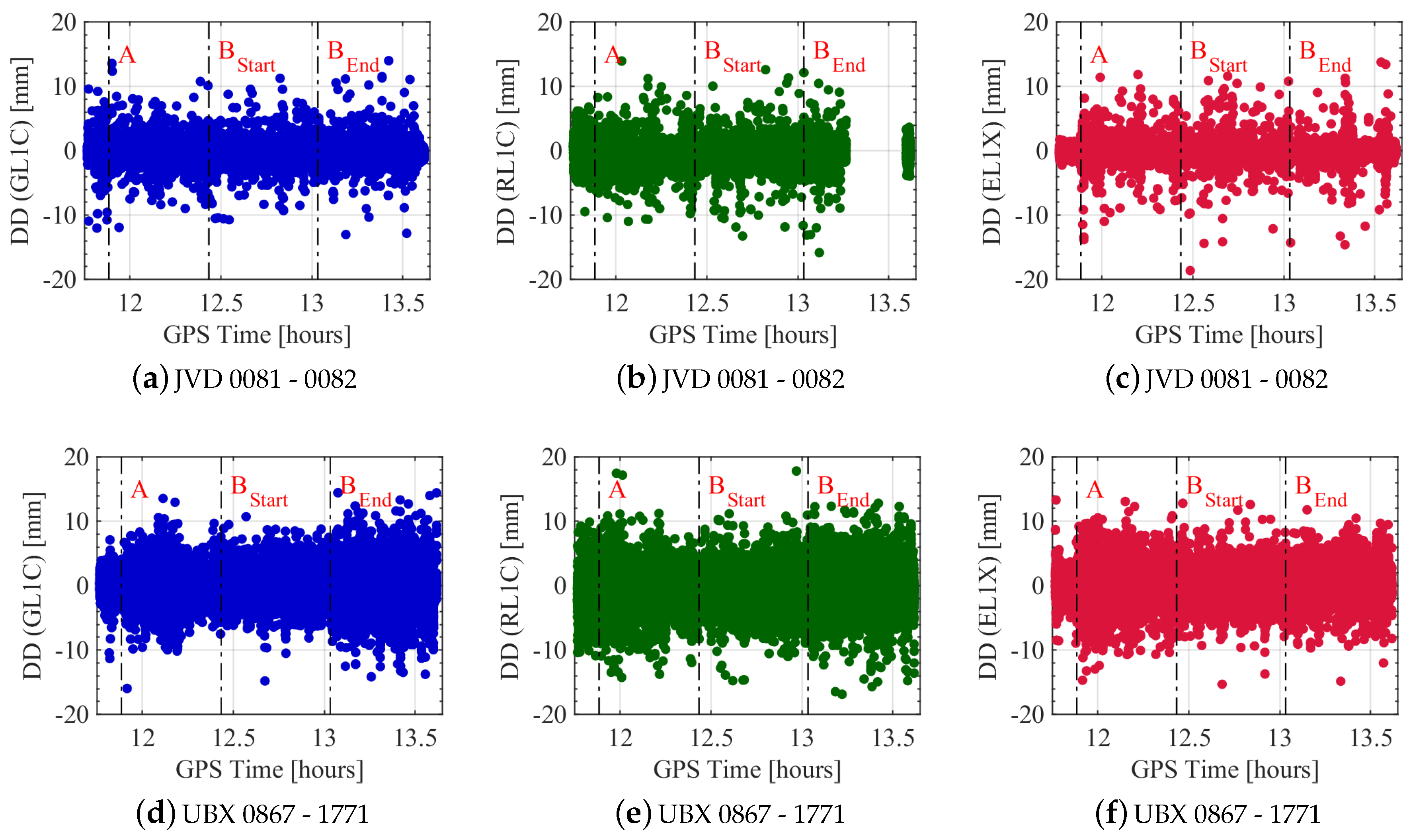
Figure 8 shows the L1 carrier phase noise of GPS, GLONASS and Galileo with respect to GPS time. The DDs of the geodetic-grade combination are depicted in the upper row while the DDs of the high sensitivity combination are depicted in the lower row. The DD noise of the different systems does not differ very much and vary roughly between ± 2 mm (
Figure 8a,c). However, there are many outliers of up to 15 mm, which affects the time series. The same applies to the DDs of the UBX receivers. The major difference is the general magnitude of noise, which is more than doubled to roughly ± 5 mm.
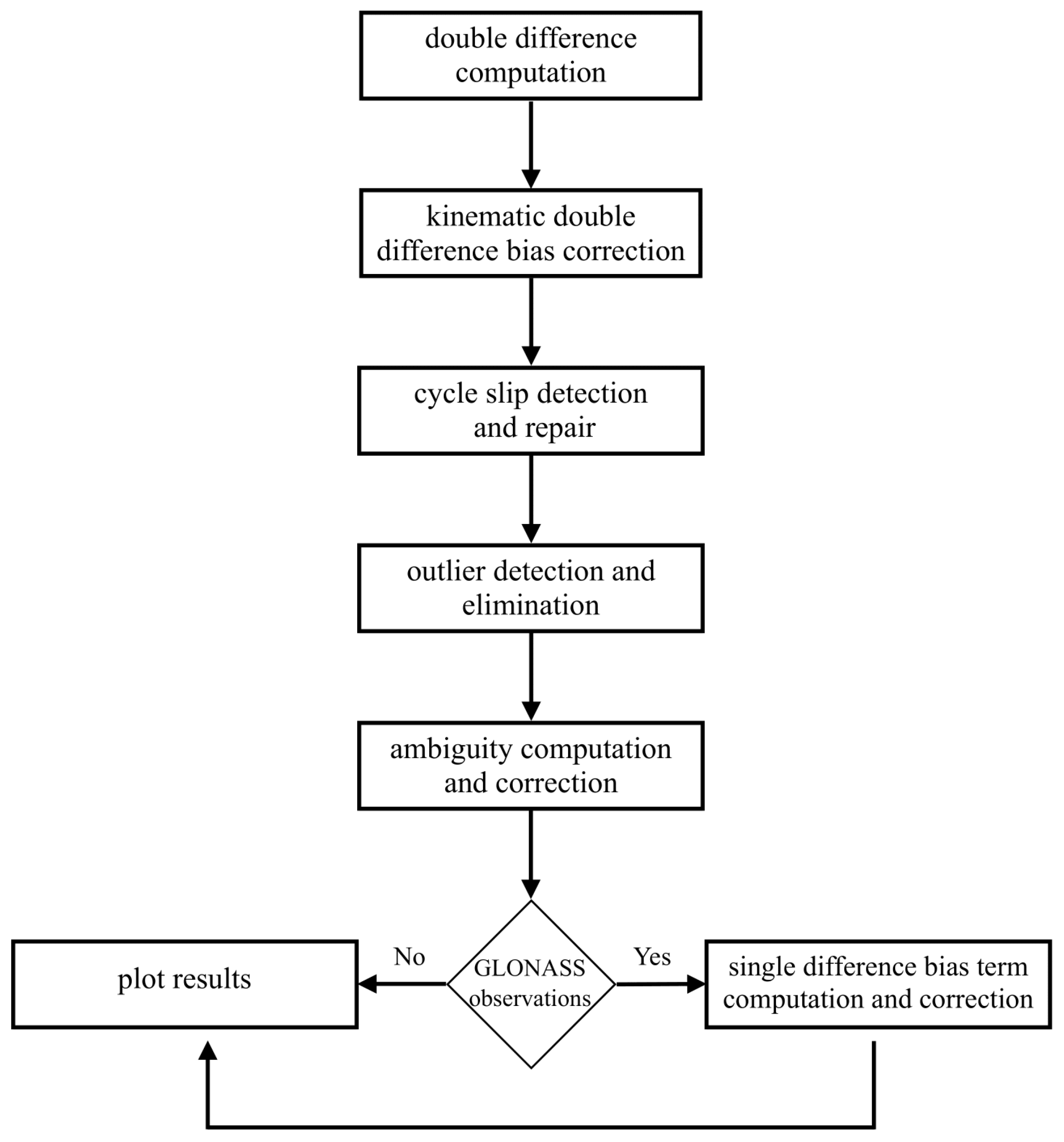
The data gap in the GLONASS time series in
Figure 8b results from the single difference bias computation (cf.
Section 3). The integer DD ambiguity can be estimated if the bias term is smaller than 0.1 cycles. In order to keep the bias term smaller than 0.1 cycles, the single difference ambiguity must be known with an accuracy of 285 cycles for the minimum wavelength difference between two satellites. Similarly, this ambiguity must be known with an accuracy of 12 cycles for the maximum wavelength difference between two satellites [
37]. This requirement for determining the single difference bias term is not met at these epochs and hence, a further analysis of the DD is not feasible. This is the reason why they are simply deleted.
Additionally noticeable is that fewer outliers appear for GPS and Galileo DDs in the stand still phase of the vehicle, which is the time until the first vertical line labelled with A. Also, the noise is lower in the static phase of the experiment. However, this does not apply to GLONASS DDs. During the repeatedly driven five rounds of the trajectory between labels B and B, neither a change in the noise level nor in the appearance of outliers is visible.
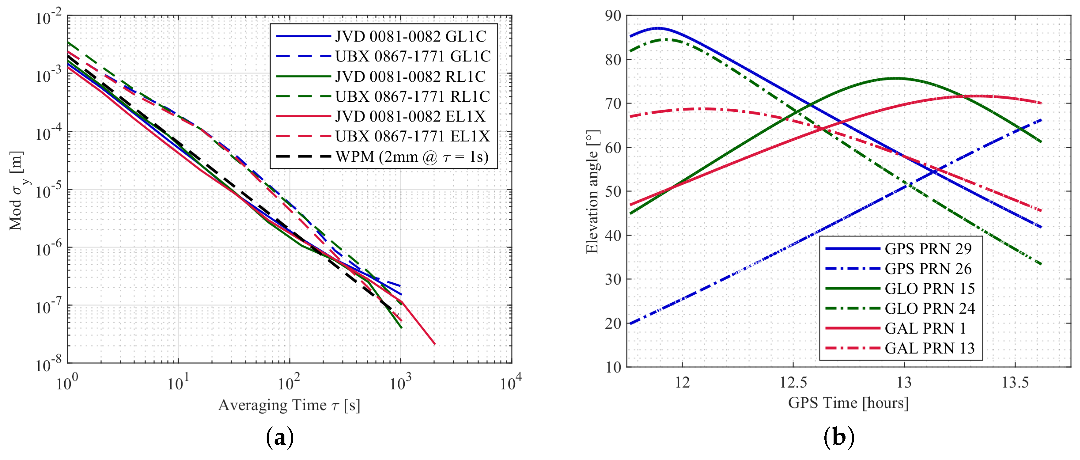
The noise characteristics of the DD time series are analysed using the Allan deviation (ADEV), which is the square root of the Allan variance [
39,
40]. To be more precise, the modified ADEV
is computed as it can distinguish between white phase noise and flicker phase noise. Since the ADEV is computed for continuous time series and this data set includes many data gaps due to signal interruptions, the DD time series from one satellite pair per system, which is almost continuous, is selected for this analysis. The modified ADEV’s are depicted in
Figure 9a. The corresponding elevation angles for these satellite pairs with respect to GPS time is shown in
Figure 9b. The noise level can be obtained at
[s]. The modified ADEV supports the statement that the noise level of the DD time series of the UBX combination is higher compared to the JVD combination; this applies to all the systems. At
[s], the values for the DDs of the geodetic combination is even below 2 mm. The slope of the respective curves is an indicator for the underlying noise process. For all combinations and signals, a white noise process for the carrier phase DDs with a slope of
is indicated in the figure for at least the first 100 s.
In order to carry out the stochastic analyses of the DDs, the computed DDs are investigated with respect to the elevation angles of the non-reference satellites (cf.,
Figure 10). A clear elevation dependency, which can be expected at least in static experiments, is not visible in any of the combinations and GNSS systems. Especially, the Galileo DDs of the JVD receivers show properties of even higher noise and more outliers for elevations between 30
and 60
. This is due to the fact that this range of elevations is particularly critical. It is shown in [
41,
42] that most of the signal reflections occur in these elevation ranges due to the building heights in the immediate vicinity of the antenna.
Since the magnitude of the DD noise is not particularly elevation dependent, the C/N
is considered as another measure to characterise the observation quality. The results are depicted in
Figure 11. Note that the x-scaling is different for the different receiver combinations. The behaviour of the DD noise with respect to the C/N
values of the non-reference satellites highly differs considering one receiver combination with the other. For the geodetic-grade combination (cf.
Figure 11a–c) there is a high C/N
dependency visible. The DD noise is increasing for low C/N
s and is decreasing when the C/N
s are increasing. This applies similarly for all three GNSS systems. Note that due to receiver-internal settings, the recording of observations is stopped when the C/N
is roughly less than 20 dB-Hz. The behaviour of the DD noise of the UBX receivers with respect to C/N
is shown in
Figure 11d–f. Note that the resolution of the C/N
is only 1 dB-Hz. A clear C/N
dependency is hardly visible. The receivers are well-known as high sensitivity equipment as it has the capability of tracking more signals even if the ray is blocked from buildings. Looking at
Table 5, this is underlined for code ranges on all L1 frequencies. The number of recorded code observations is always higher compared to the geodetic-grade receiver. Investigating the carrier phase observations on the same frequencies, the numbers reveal an opposite behaviour in most cases.
Depending on the GNSS system analysed, the UBX receivers are recording 17% to 26% less carrier phase than code observations while the JVD receivers are recording the exact same number of code and phase observations. The computed DDs are in the C/N range of 25 to 54 dB-Hz, which leads to the assumption that the analysed UBX receivers are not capable of continuously tracking carrier phase observations in challenging situations and low C/N scenarios.
Figure 12 depicts the cumulative distribution functions (CDFs) for carrier phase DDs on different frequencies. Investigating the JVD DDs, 95% of the values for GPS, GLONASS and Galileo are below 2, 2.8 and 1.7 mm, respectively. For the UBX DDs, 95% of the values for GPS, GLONASS and Galileo are below 4.8, 5.6 and 4.7 mm, respectively. To get an idea of the quality of the carrier phases on the other frequencies, the CDFs of L2 frequencies and L5 frequencies are shown in
Figure 12b,c. This is only feasible to analyse with the JVD combination, since the UBX receivers were tracking only one frequency. Compared to the L1 results, the quality of L2 and L5 DDs are relatively poor. For GPS and GLONASS L2 DD, 95% of the values are less than about 3.6 and 5.3 mm, respectively. For GPS and Galileo L5 DD, 95% of the values are below 4.8 and 3.8 mm, respectively. These results underline that the quality of GPS and Galileo carrier phase observations are similar, whereas the quality of GLONASS carrier phase observations is worse in comparison.
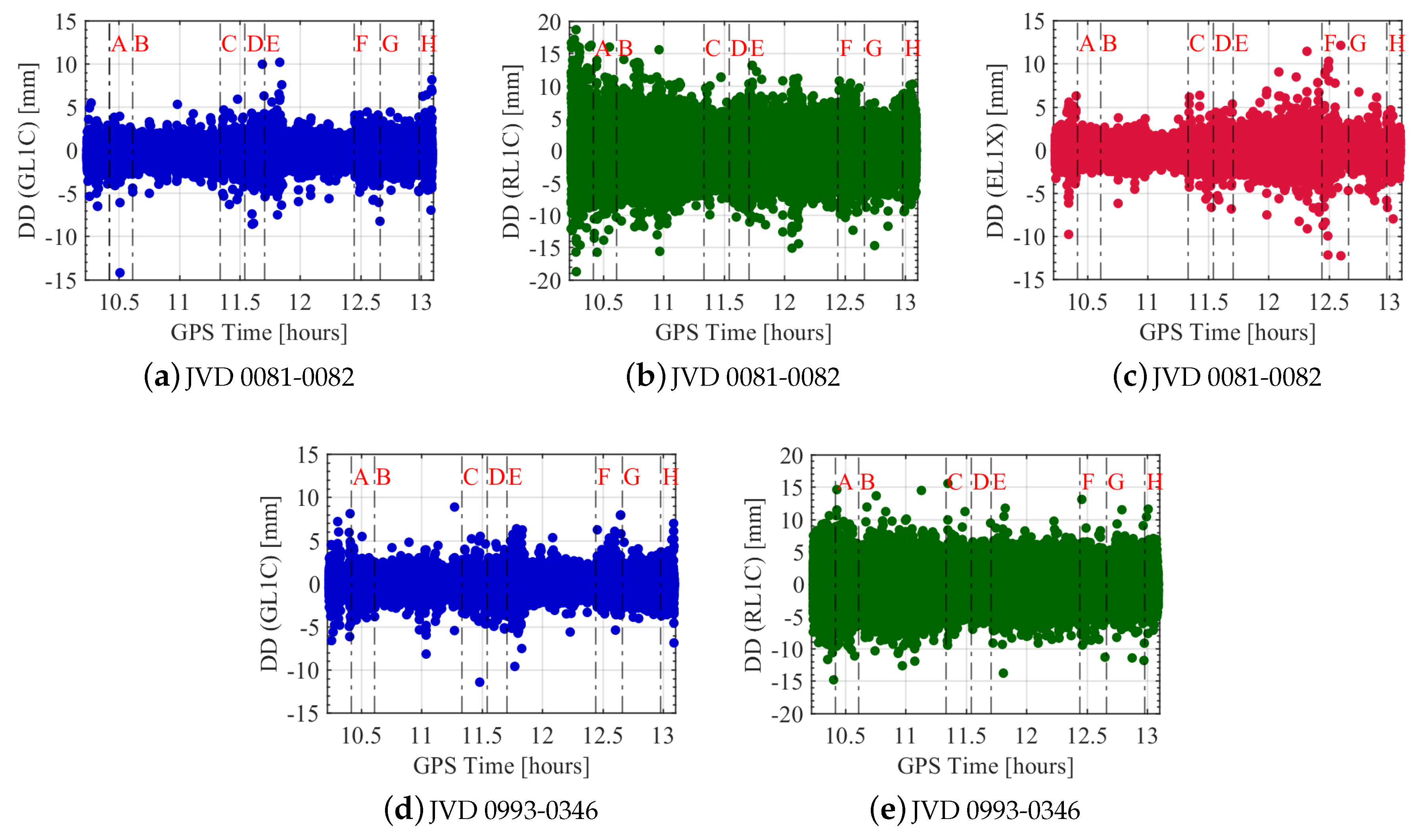
4.2. Flight Test Case
All the following analyses concerning the flight experiment were carried out using two receiver combinations operating in zero-baseline mode. The first combination is between JVD receivers 0081-0082, both of which are connected through external atomic clocks while the second combination is between JVD receivers 0993-0346, wherein receiver 0346 is driven through its internal TCXO. These two combinations were selected to observe any particular changes in the noise levels due to different clock configurations. Also, DD estimates from all the satellites in a constellation are superimposed in each subplot.
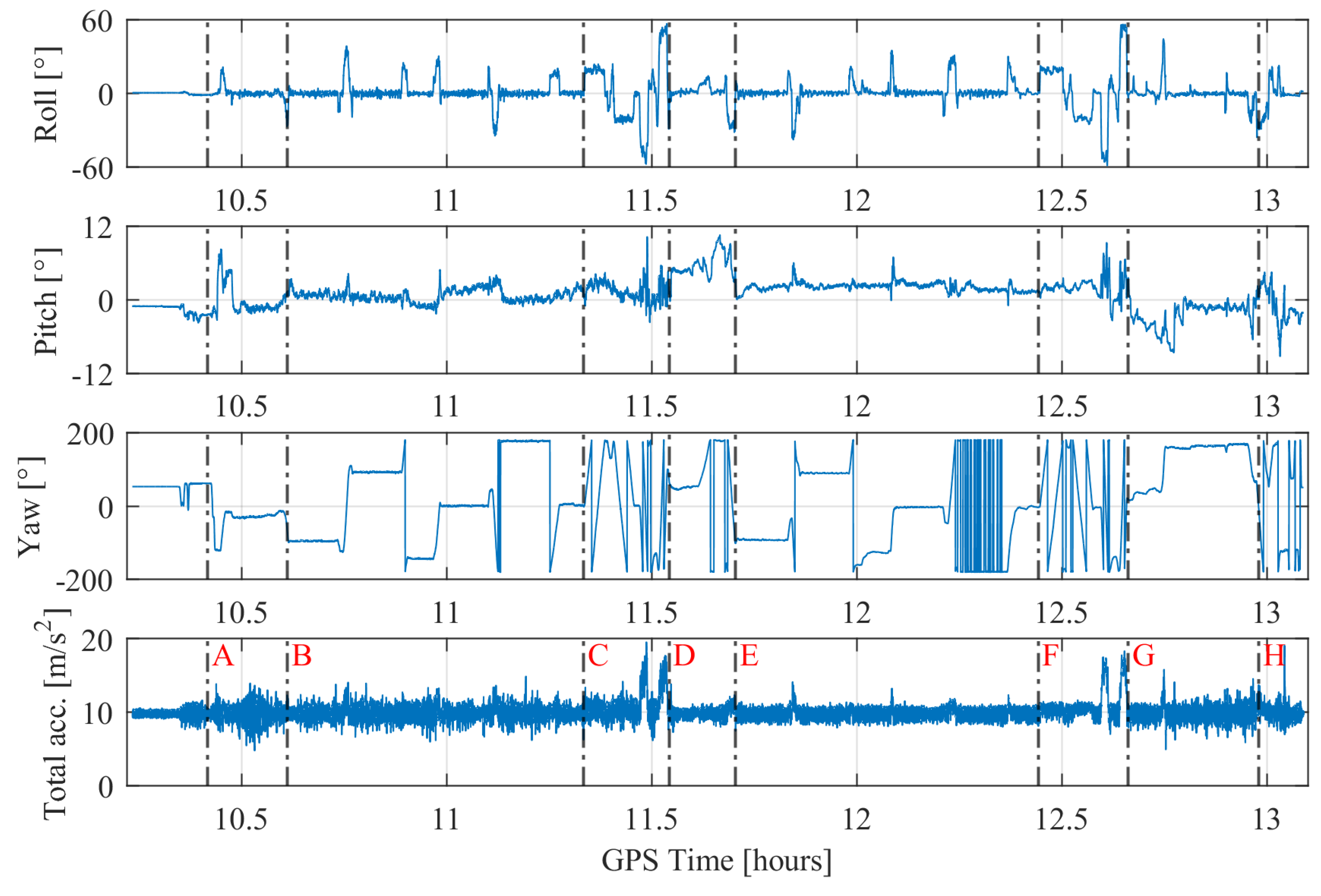
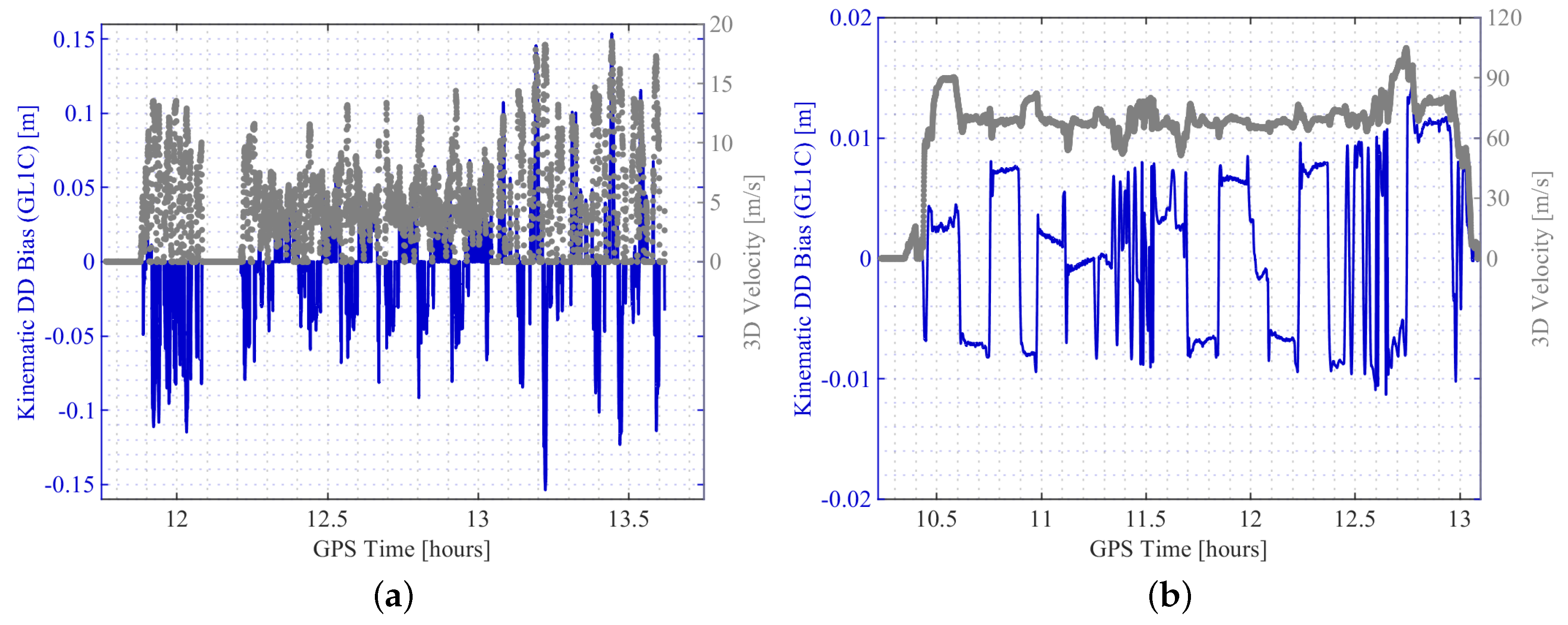
Figure 13 depicts the L1 carrier phase DDs of the moving zero-baseline for GPS, GLONASS and Galileo with respect to GPS time. They are computed as explained in
Section 3. The GNSS system specific (GPS and GLONASS) noise dispersion are almost similar for both the receiver combinations, except that the number of outliers for the first receiver combination is higher for GLONASS observations compared to the second receiver combination. This is mainly due to the large number of outliers deleted for the second receiver combination during the DD estimation process compared to the first (cf.
Table 4). Apart from a few outliers, the deviation of GPS L1 carrier phase is about 2 mm for the complete flight trajectory. In the case of the GLONASS L1 carrier phase, the noise is slightly higher during the start of the flight experiment (segment: start-A) compared to the other flight segments of the first receiver combination. During the segment (start-A), the aircraft was static for about 6 min and then was moving at a low velocity towards the runway. Along the complete trajectory, the sudden noisy spikes seen correspond to the flight turn, which resulted in a change of flight roll and heading angles. Overall, the deviation for GLONASS is about 5 mm for both receiver combinations, which is 2.5 times higher compared to GPS. For the first receiver combination, the spread of Galileo L1 carrier phase noise is about 2 mm for the complete flight trajectory, similar to GPS. It is also seen that the values of Galileo L1 phase noises are slightly higher at the upper altitude (segment E-G) compared to those at a lower altitude (segment A-D). Finally, there are no GNSS system specific significant changes that are seen in the computed noise levels during the highly dynamic manoeuvres (segments C-D, F-G).
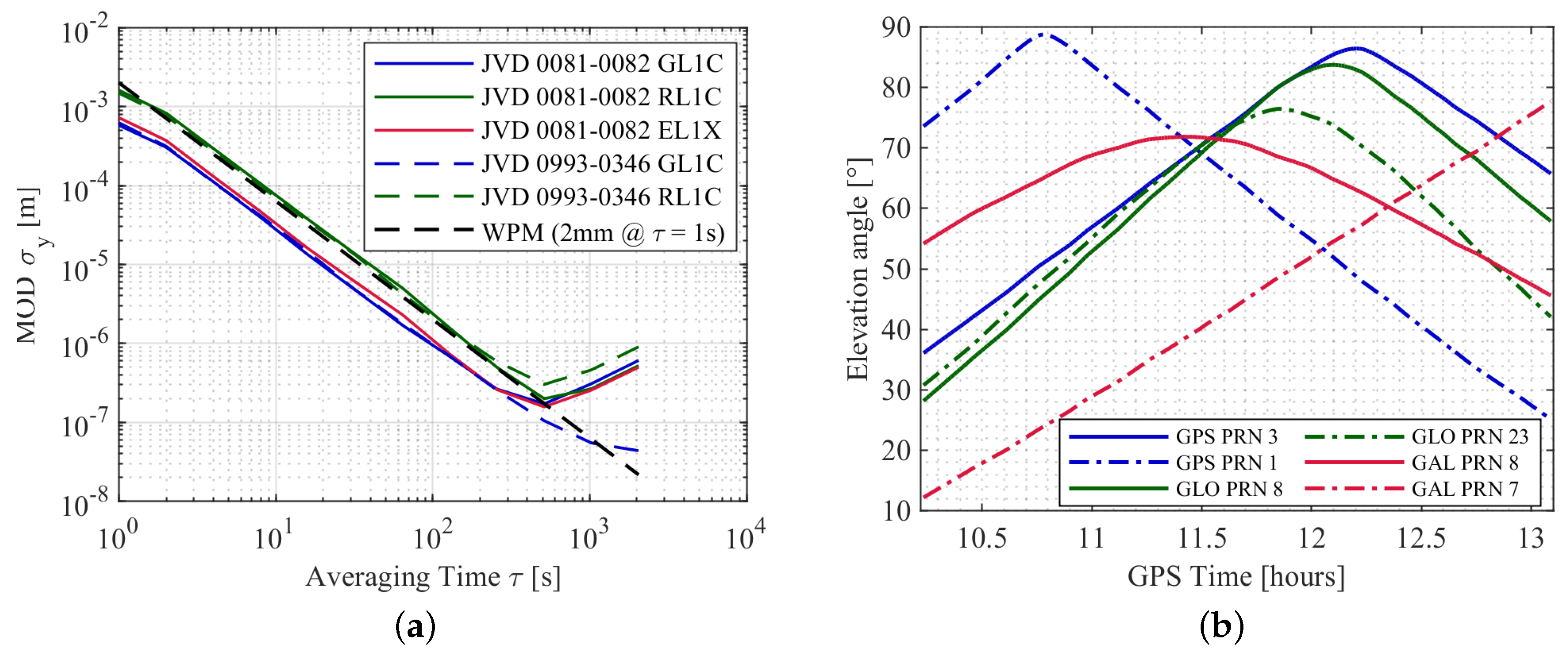
Similar to the urban case, the underlying process noise of the carrier phase observations are analysed with the modified ADEV’s. The estimated DDs from one satellite pair of each GNSS system and two different receiver combinations are used to compute the modified ADEV’s and are shown in
Figure 14a. The corresponding elevation angles of the different satellites are depicted in
Figure 14b. It is seen that the noise process of L1 carrier phase observations from different systems resembles largely white phase noise (WPM) for up to
[s]. Moreover, receiver combinations with different clock configurations does not have a large impact on the quality of the observations. Also, the higher noise level of the GLONASS L1 observation is clearly visible compared to GPS and Galileo L1.
The stochastic behaviour of GNSS L1 carrier phase DDs is analysed in connection with satellites elevation angles and the received C/N
of the corresponding signals.
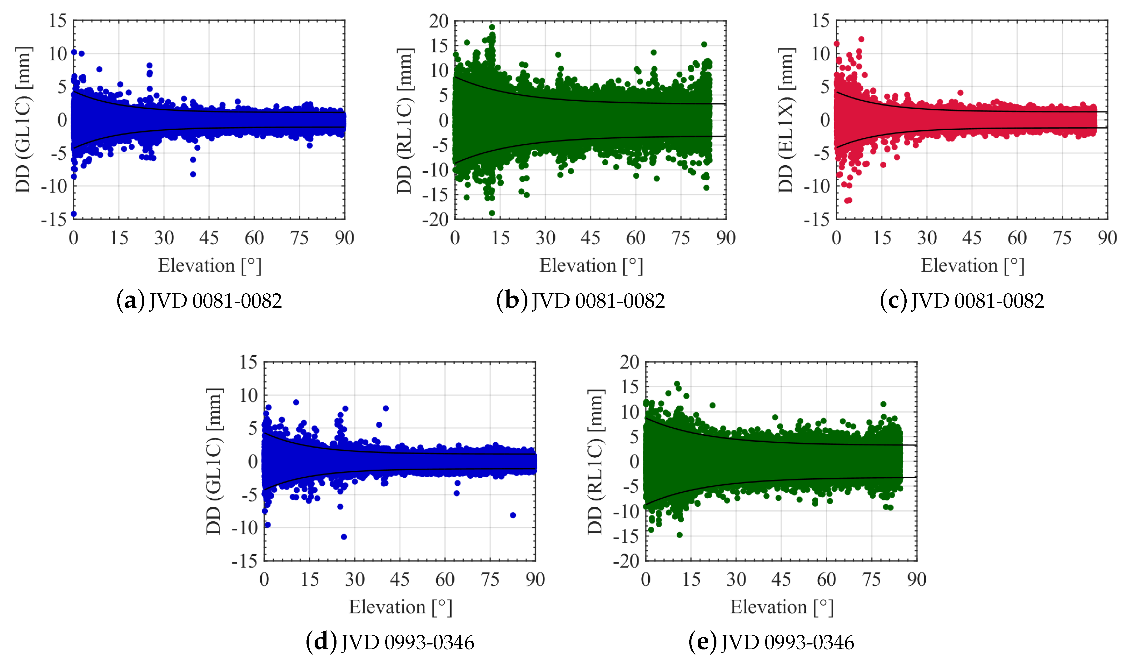
Figure 15 shows the DDs for GPS, GLONASS and Galileo L1 carrier phases with regards to the satellite elevation angles. All the sudden spikes observed in computed GNSS DD at elevation angles greater than about 10
are due to recorded data from an ascending satellite or just before the loss of visibility of a satellite already in view. An elevation dependency is observed for all the computed DDs. The standard deviation of the phase range dependent on the elevation angle
h can be approximated using the following exponential function [
13]:
where
,
are constant terms;
represents the scaling factor for the elevation angle. The values listed in
Table 6 are derived empirically to model all the estimated L1 carrier phase system specific DDs with all the receiver combinations. As examples, decreasing exponential functions for two different receiver combinations evaluated using the parameters in
Table 6 can be seen in all plots of
Figure 15. The corresponding increasing exponential function seen in
Figure 15 is equivalent to a change in the sign of decreasing exponential function. From
Figure 15, an elevation dependent weighting scheme modelled as an exponential function is justified for aerial navigation applications requiring higher accuracy and precision.
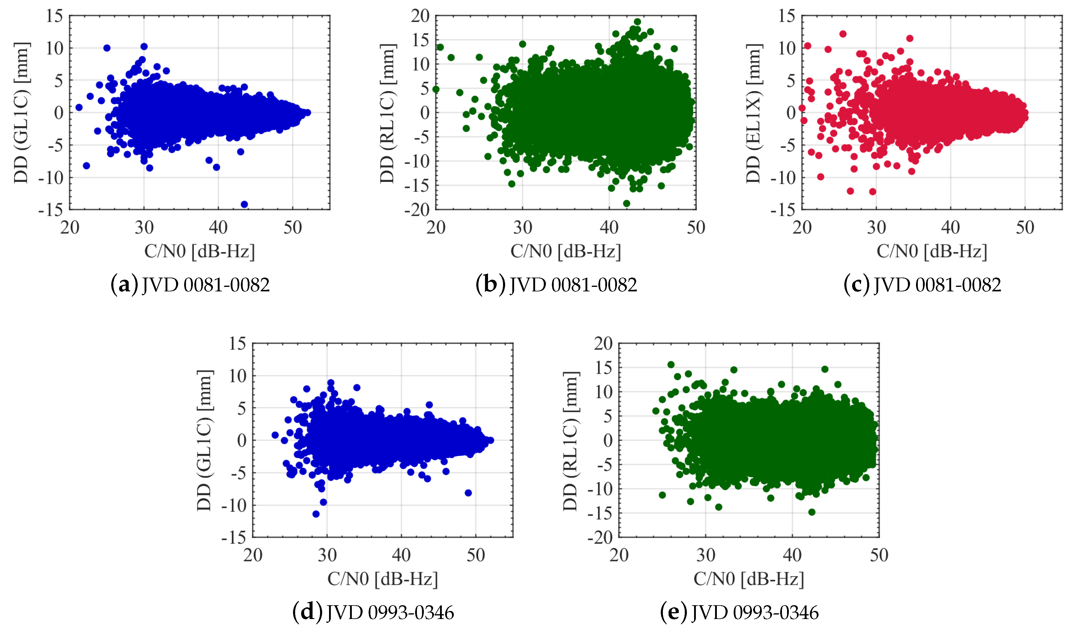
The DDs for GPS, GLONASS and Galileo L1 carrier phases in relation to the received signal’s C/N
from different satellites are shown in
Figure 16. It is observed that the behaviour of GPS L1 DDs is similar for both the receiver combinations. In the case of GLONASS, the DDs varies largely randomly with the C/N
and no correlation is observed for both receiver combinations. A C/N
dependency is visible for GPS and Galileo, wherein large C/N
leads to smaller noise levels in most cases and vice versa. As explained in the elevation dependency scenario, few outliers seen at large C/N
are due to the addition of a new visible satellite or loss of visibility of a satellite during the experimental campaign. Based on the analysis, a C/N
dependent weighting scheme is also suitable for GPS and Galileo L1 phase observations in aerial applications.
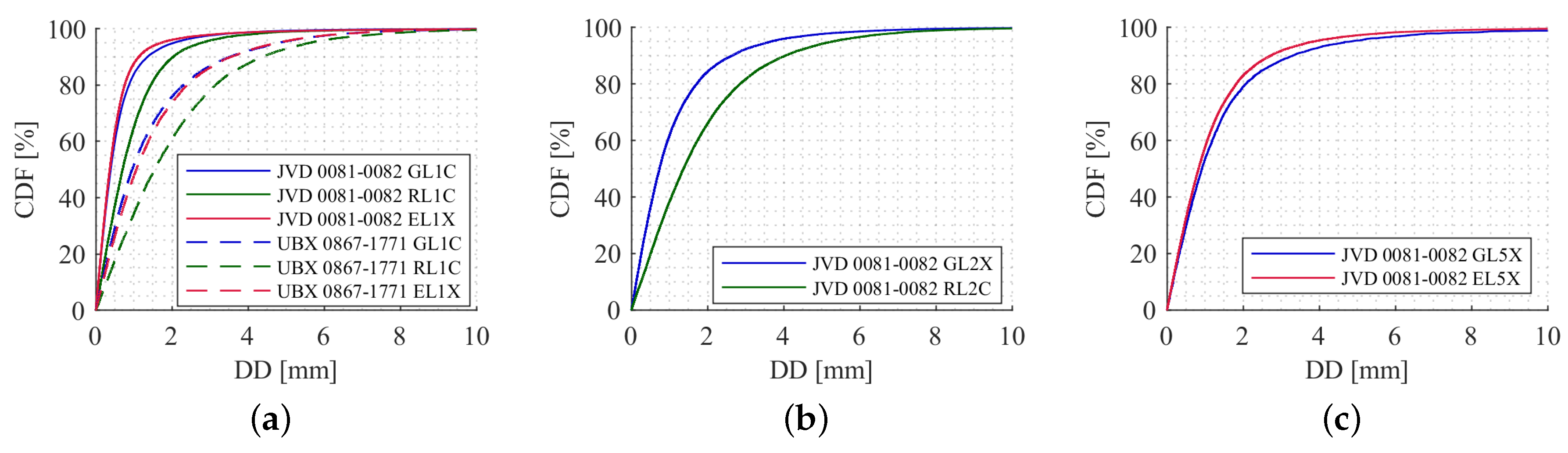
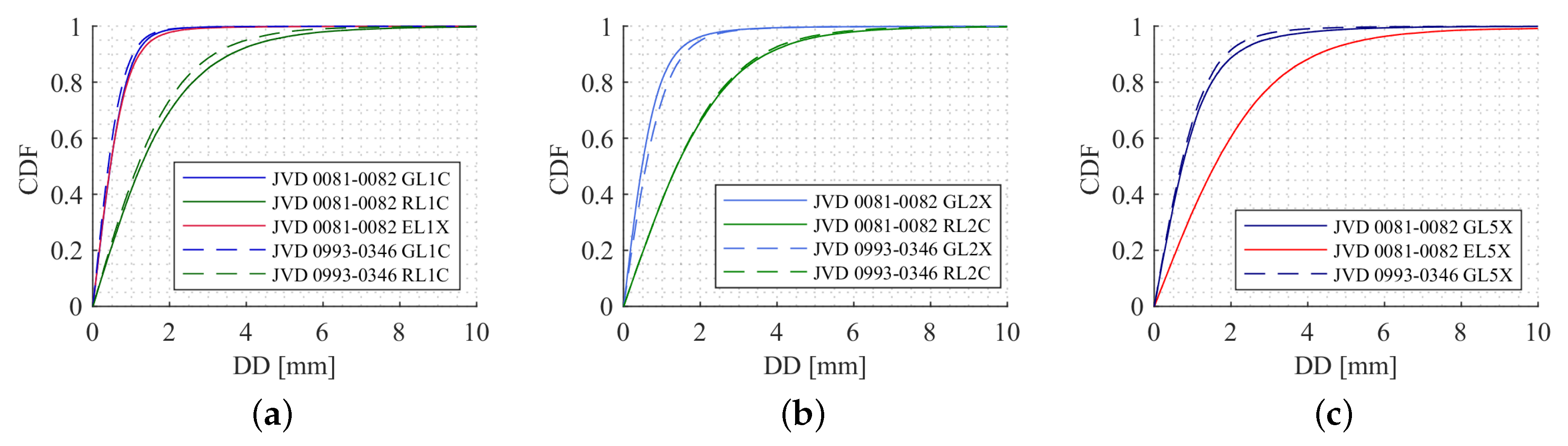
In order to see the noise behaviour of L2 and L5 carrier phase observations alongside L1, DDs are computed and analysed using CDFs.
Figure 17a–c shows the CDF for L1, L2 and L5 carrier phase observations, respectively. For both the receiver combinations, 95% of the DD values for GPS, GLONASS and Galileo L1 are less than about 1.4, 4.6 and 1.5 mm, respectively. Similarly, for GPS and GLONASS L2, 95% of the DD values are less than about 2 and 4.7 mm, respectively. Finally, for the GPS and Galileo L5 observations, 95% of the DD estimates are less than about 2.8 and 5.4 mm, respectively. For other receiver combinations, the noise levels are almost similar with regards to L1, L2 and L5 carrier phase observations. Even though the noise level is slightly higher for both L1 and L2 GLONASS DDs, the values are acceptable in the case of kinematic data processing. There is a significant increase in the noise level of Galileo L5 observation when compared to its L1 data-set.


