Prediction Corrections
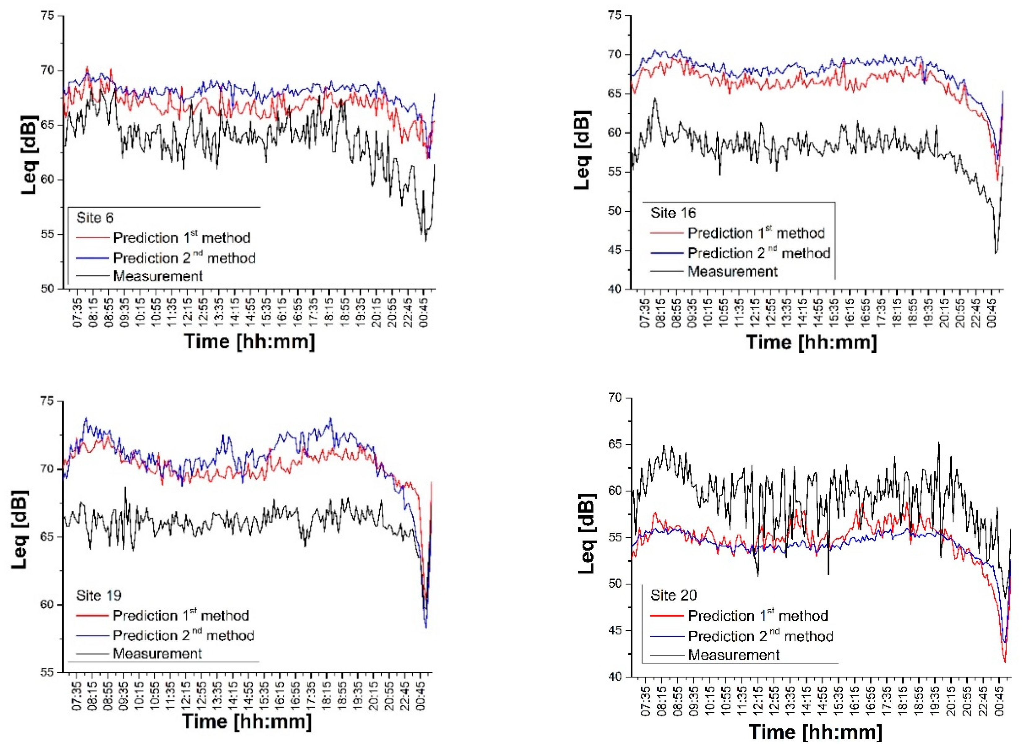
A number of selected sites have been chosen to compare the results of field measurements with the corresponding DYNAMAP predictions.
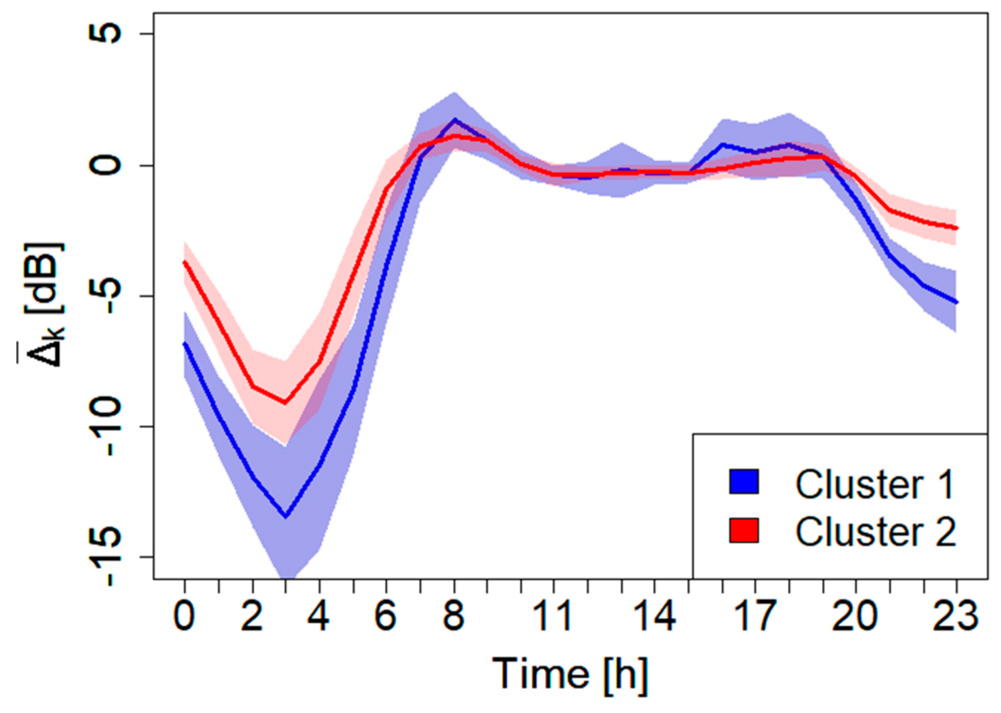
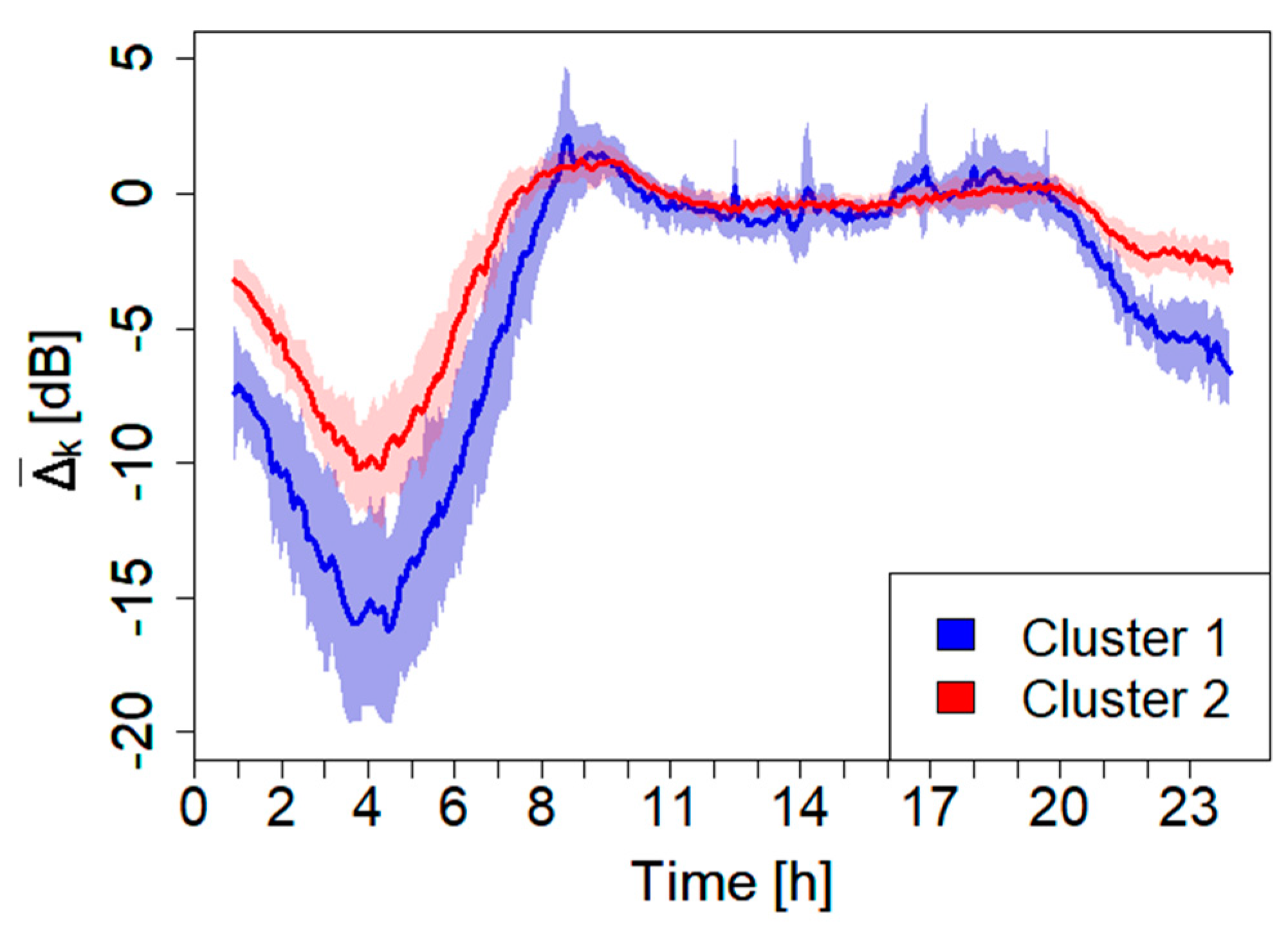
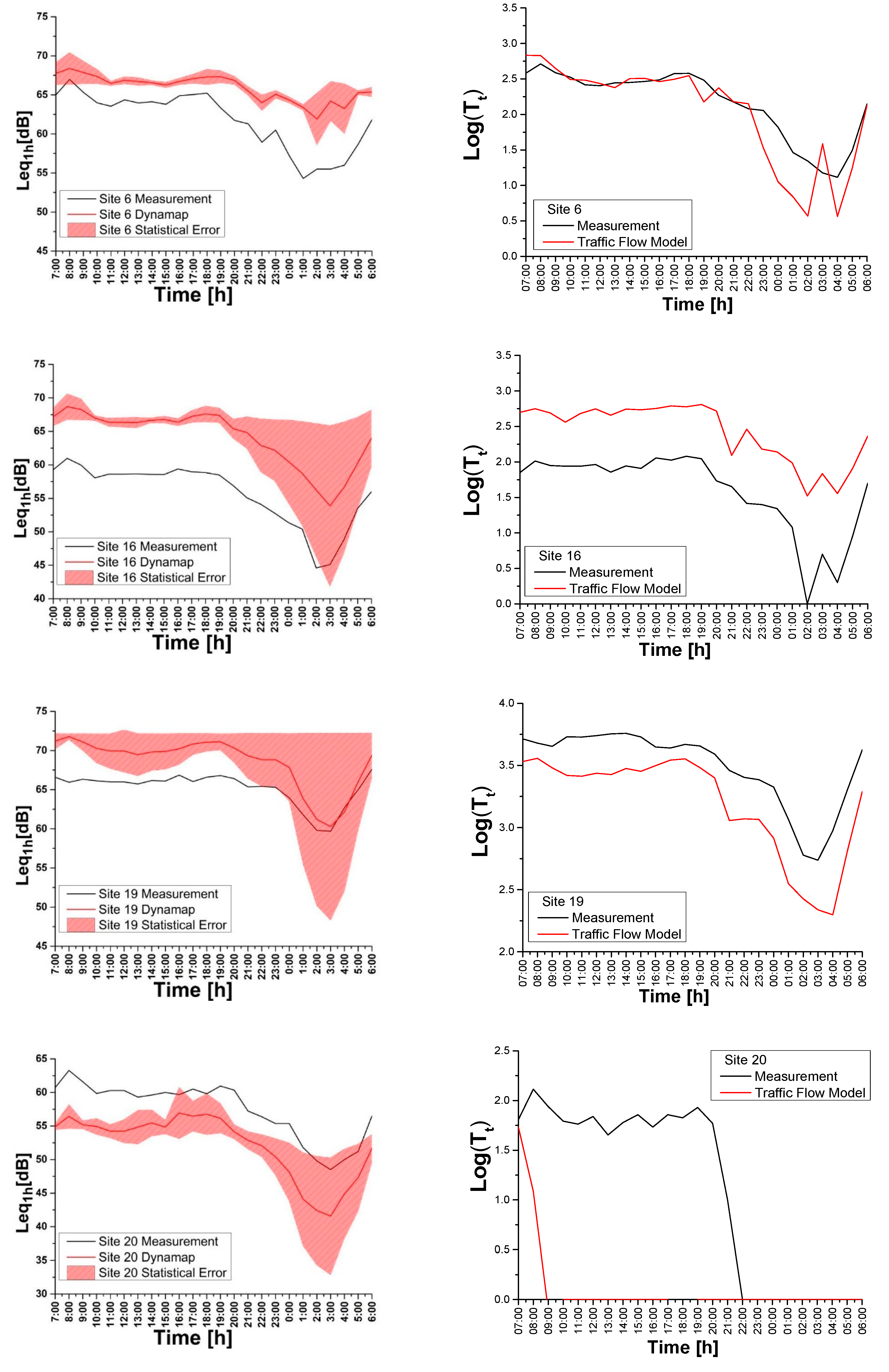
Figure 14 (left part) presents a relevant discrepancy between predictions and measurements, which can be higher during the daytime. Each figure shows the error bands obtained from the propagation error associated with the variability of
within each group
g. During the day time (07:00–21:00) the mean group discrepancy remains within 1 dB, whereas in the evening-night time (21:00–07:00) the high “volatility” of traffic noise pushes it to about (2–4) dB.
The almost constant gap between measurements and predictions in different period of the day suggested us to search for a systematic error inherent the DYNAMAP calculation method; systematic error which is most likely correlated to the vehicular flow employed in the prediction model. In fact, is calculated with respect to Leqref g, obtained from CADNA software using as input information on the number of vehicles/hour at the reference hour (8:00–9:00).
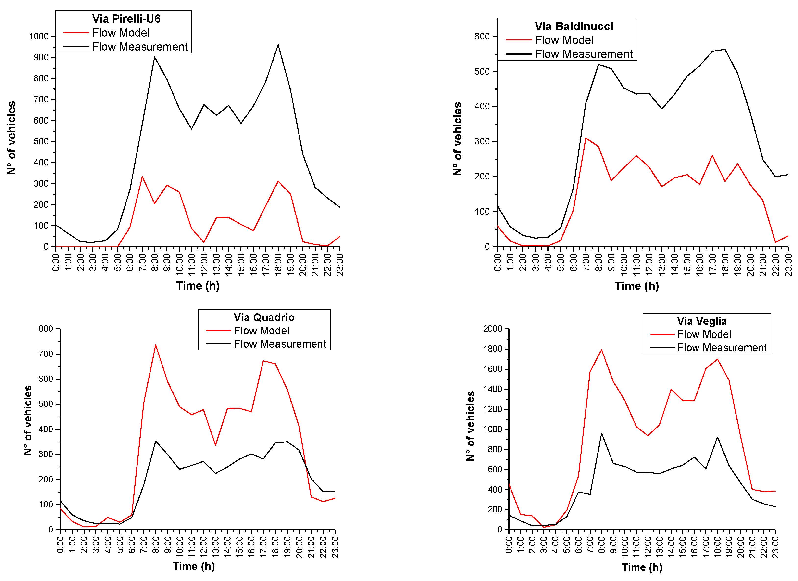
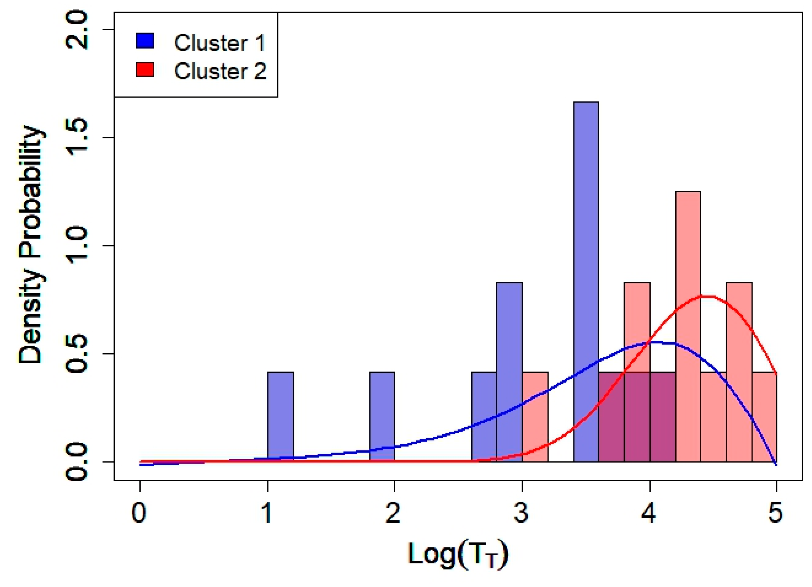
During the measurement campaign, we simultaneously recorded the traffic flows. This allowed us to compare the logarithm of traffic flow measurements with the traffic flow model calculations for Sites 6 (
g3), 16 (
g4), 19 (
g6), and 20 (
g1) as illustrated in
Figure 14 (right part), respectively. The traffic flow data have been provided by Agenzia Mobilità Ambiente Territorio (AMAT), the agency in charge of the traffic mobility at the City Hall [
46]. In the described examples, the model yields more reliable results for highly traffic roads belonging to groups
g3,
g4, and
g6, than for lower flow roads as in
g1, as already reported in a previous preliminary work [
45].
As it is apparent from
Figure 14, there is a gap between the prediction and the measurements of
. The observed constant shift might be the result of inaccuracies of the traffic model in describing the traffic flow, especially for low traffic roads. Such shift is regarded as a systematic error.
To quantify this discrepancy and try to correct it, we calculate for each site the relative mean deviation (
εL) between hourly traffic noise measurement level,
, and the corresponding hourly DYNAMAP prediction level,
, over the day and night period, defined as
where the summation index
k extends over two time zones (day 07:00–21:00 h →
N1h = 14; evening-night 21:00–07:00 h →
N1h = 10). The relative error is then averaged over all roads belonging to the same group, in order to represent the average hourly values of the road group (
). Furthermore, we consider the relative deviation (
εF) between measurement and model for the logarithm of the traffic flow at the reference time,
Log F(8:00–9:00),
where
Log(
F(8:00–9:00)Model) is the logarithm of the flows from 8:00 to 9:00 of the 2012 traffic model. Then we calculate the mean deviation of all sites belonging to the same group,
.
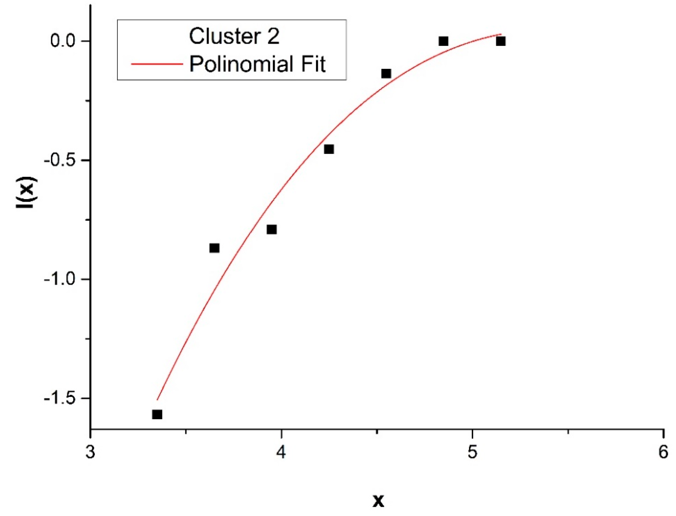
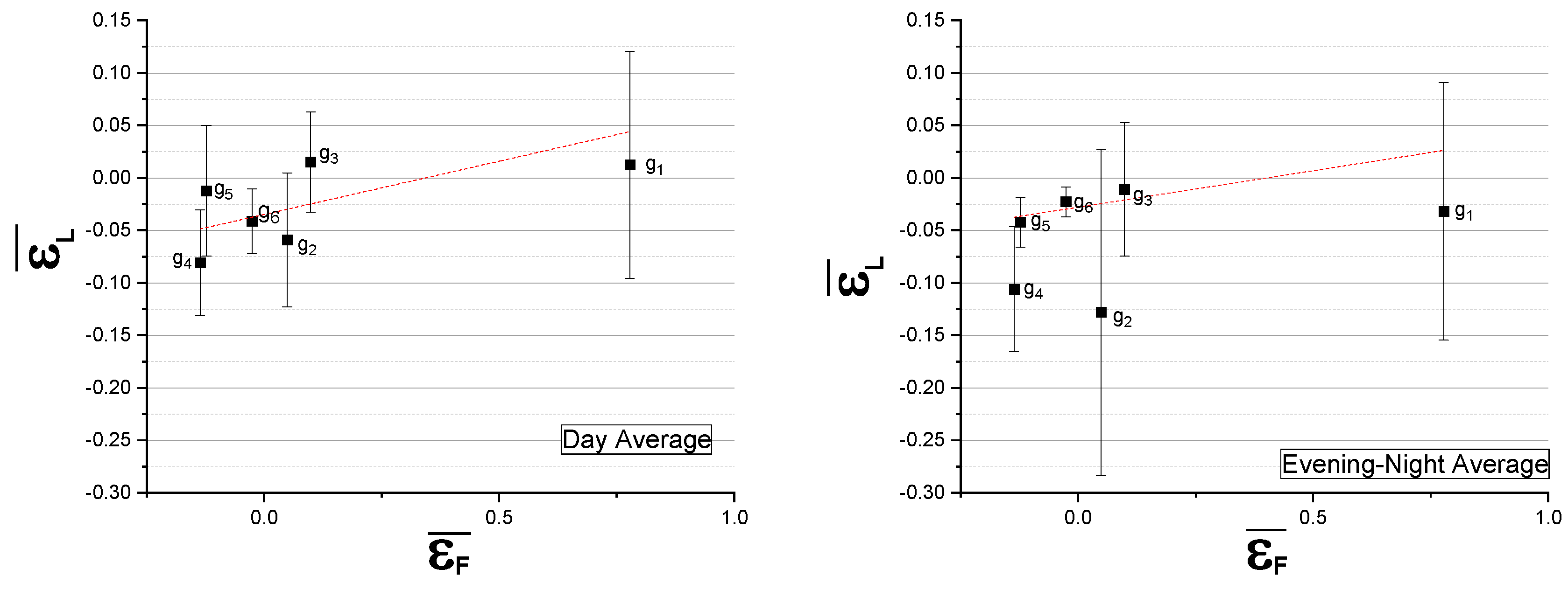
These values for
and
are plotted in
Figure 15, illustrating, to some degree, a relationship between traffic flow deviations and noise level errors. This relationship will be treated as a systematic error and taken into account within the DYNAMAP scheme.
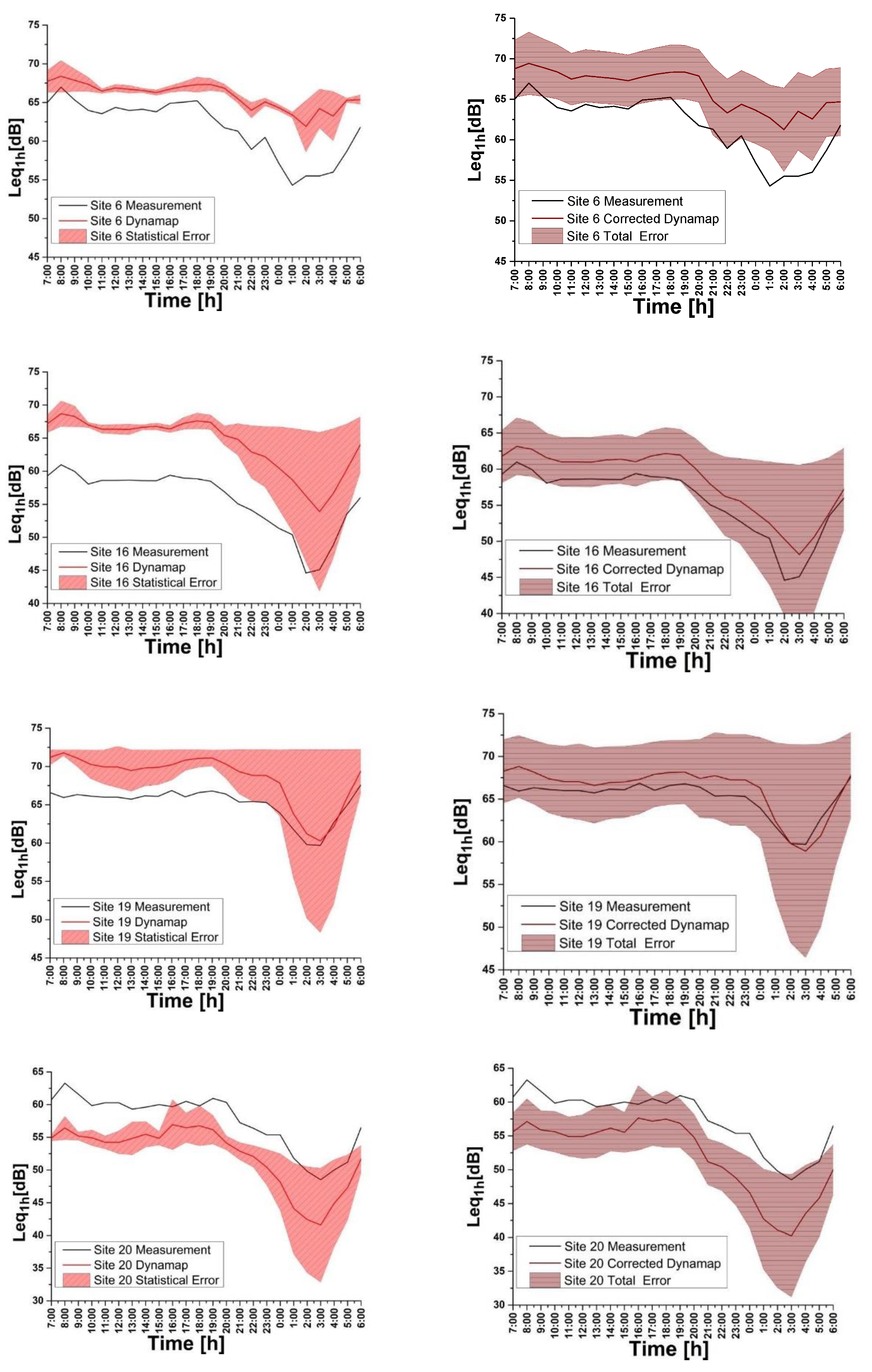
We thus obtain the corrected hourly value for the predicted noise level (
), by multiplying the different hourly values of the predicted noise level times the relative mean group deviation, expressed in percentage terms [1 +
(
g)]. The results of this operation are shown in
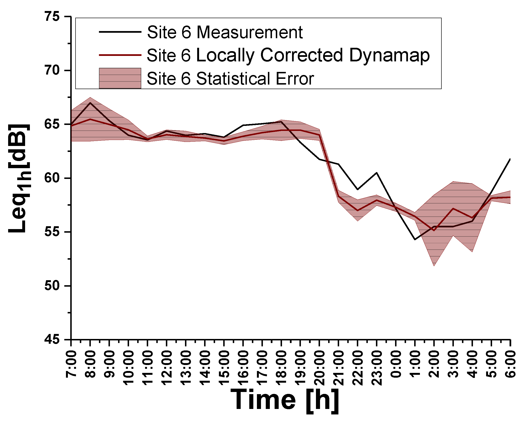
Figure 16 (Right part, red line). We observe a general improvement of the prediction for these sites. In the graphics, the uncertainty bands include both the statistical and systematic errors (total error).
In
Table 8, we report both the site mean hourly non-corrected,
<εLeq>N, and corrected prediction errors,
<εLeq>C, for all measurement sites, obtained through the comparison between the hourly non-corrected or corrected prediction levels and the hourly measurement levels, as shown in Equation (12).
The correction yields better predictions in many cases, but in others it remains poor. A median-based correction,
<εLeq>M, is also reported in
Table 8. This quantity is less sensitive to outliers and, consequently, it provides more realistic estimates of the corrections. Finally, the right column of
Table 8 shows the group mean errors calculated by averaging over the roads belonging to each group. The highest discrepancies are found for group
g1 as a consequence of the poor descriptive capabilities of the traffic flow model. Except for this, the results obtained for the group median-average error,
<εLeq>M, is below 3 dB.
Therefore, excluding group
g1, for which a specific analysis needs to be developed, the prediction error of roads belonging to other groups, upon a systematic error correction
<εLeq>C, remains below 3 dB for each site, with the exception of Sites 6 (
g3) and 7 (
g2). The latter must be treated differently if we require that the 3 dB constrains must apply to all sites belonging to a group. We took 3 dB as a reference accuracy value as retrieved from the Good Practice Guide for strategic noise mapping [
47]. As an example, consider site 6 (
g3). Correcting the predicted noise level using its own relative traffic flow deviation (not the group mean), we obtain the results reported in
Figure 17, that correspond to
<εLeq>C = 1.1 dB.
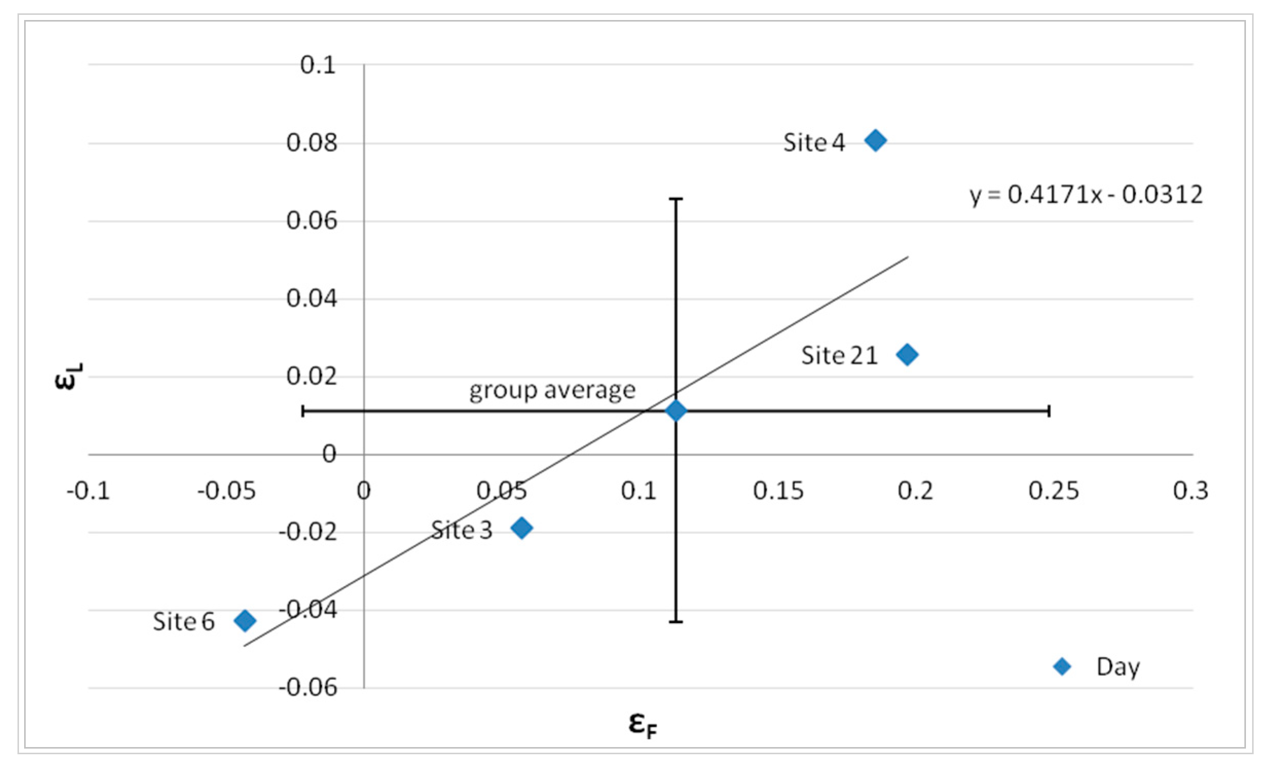
This result suggests that in order to get an effective correction, the relative error between the measured and the model traffic flow (8:00–9:00) in a given road stretch has to be bound within an interval that depends on the group it belongs to. In
Figure 18, for example, we report the relative mean hourly deviation between traffic noise measurements and the corresponding DYNAMAP predictions,
εL, against the relative deviation between the logarithm of traffic flow measurements and the corresponding model calculations at the reference hour (8:00–9:00),
εF, for each site of group
g3.
Figure 18 has been obtained assuming for simplicity that the relation between
εL and
εF is linear within group
g3. In this case, in order to get a prediction error <3 dB for each site, the relative error on the traffic flow can vary by about ±0.10 with respect to the minimum found for the single site, as it can be observed in
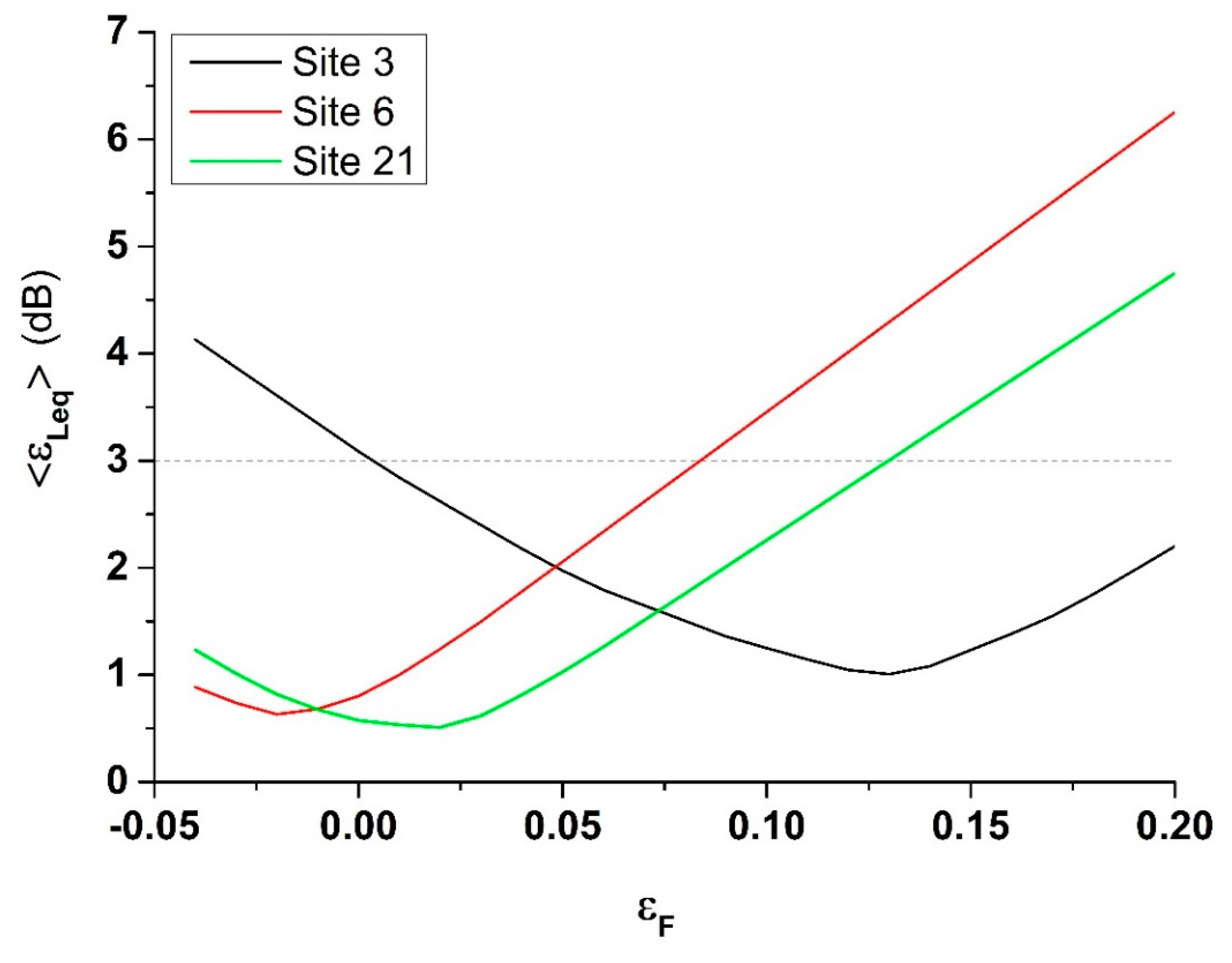
Figure 19 for Sites 3, 6, and 21.
In
Figure 19, the minimum prediction error is obtained near the corresponding site-specific flow error. It does not match exactly the value reported in
Figure 18 because we are using a linear dependence between
εL and
εF (see
Figure 18). In other words, the mean value of the relative error on the traffic flow of a given group
g,
, (the one that has been used in the correction procedure of DYNAMAP prediction) must be bound within an interval that can be determined as follows: if we take
centered at the minimum of the relative error of the site-specific traffic flow,
εF,S6m for the case of Site 6, it means that
= εF,S6m can have a maximum standard deviation σ = ±(0.10) to satisfy the condition about the mean prediction error, <
εLeq> < 3 dB. Therefore,
must belong to an interval (
εF,S6m − 0.10,
εF,S6m + 0.10). This procedure has to be repeated for each site of the group. If these conditions are met, all sites will have <
εLeq> < 3 dB. This means that the traffic model must provide flow values for the streets belonging to each group with comparable accuracy in order that the error remains within the same threshold for all sites of the group.
As for roads characterized by low traffic flows, such as those belonging to group g1, the application of the correction based only on the relative deviation of the local traffic flow is not effective, because in these cases, the noise level is not mainly determined by the local traffic, but by that of busier nearby roads. In these cases, we may think to reassign them to other groups, applying the correction of the group whose contribution in the prediction of the noise level is predominant.


