1. Introduction
The development of smart infrastructure has highlighted the need for automatic and real-time monitoring systems for critical transportation components such as bridges. The high cost associated with maintenance and reconstruction of these essential lifelines has made the implementation of such monitoring systems a pressing issue. Consequently, significant research has been conducted over the last few decades in the area of vibration-based monitoring of bridge structures using sensors installed directly on the bridges [
1,
2,
3].
Previous studies have made notable contributions to bridge health monitoring. For instance, Gonzalez and Karoumi [
4] proposed a damage detection method for bridges utilizing bridge weigh-in-motion (BWIM) data and machine learning techniques. Their approach employed an artificial neural network (ANN) to predict bridge health based on BWIM data, ensuring reliable evaluations over time. Similarly, Azim and Gül [
5] developed a data-driven damage detection framework for truss railway bridges using operational acceleration and strain response data. Feng and Feng [
6] presented a time-domain finite element (FE) model updating approach using in situ measurements of dynamic displacement responses under trainloads. Their study validated the importance of the bridge’s equivalent stiffness for accurate model updating, although extracting modal information from dynamic responses proved challenging for short-span railway bridges with high natural frequencies.
Due to the high cost of real-time monitoring of bridges using fixed sensors, recent research in structural health monitoring has explored indirect methods, called indirect bridge health monitoring (iBHM), that utilize only the vertical vibration data collected by accelerometers mounted on passing vehicles. This method, first proposed by Yang et al. [
7], has recently gained significant recognition. The main objective in this research direction is to find a reliable method to determine the vertical vibration responses of desired locations on a bridge without the need for expensive fixed sensors or with minimal sensor requirements [
8,
9]. For example, Malekjafarian and O’Brien [
10] developed a method for identifying bridge mode shapes using short time frequency domain decomposition (STFDD) of responses measured in a passing vehicle. Their approach involved segmenting the bridge and employing a multi-stage procedure using frequency domain decomposition (FDD) to estimate the mode shapes. Numerical case studies validated the performance of the method, demonstrating the accurate estimation of mode shapes under low noise levels and the presence of other traffic or signal subtraction in identical axles. Furthermore, Eshkevari et al. [
11] developed novel methods for modal identification of bridges using data collected by a large number of moving sensors (vehicles). Their study proposed matrix completion methods, specifically the alternating least squares algorithm, to extract modal properties from sparse and dynamic bridge response data. Three methods were evaluated: principal component analysis, structured optimization analysis, and the natural excitation technique (NExT). The results demonstrated accurate estimations of modal properties. However, the methods had limitations in terms of computational costs, modal leakage, sparse data, user-defined points, and accuracy for higher modes. The study showcased the potential of using mobile sensor networks for bridge health monitoring and system identification. Kong et al. [
12] proposed a method to efficiently extract bridge modal properties using a test vehicle composed of a tractor and trailers. They verified the method on an existing bridge, considering the effects of trailer mass and stiffness. Their findings demonstrated high visibility in extracted bridge frequencies, particularly when traffic flows provided additional excitation. However, limitations were identified, such as difficulties in accurately extracting mode shapes dominated by lateral bending due to the limited modeling of trailers.
To reduce the cost of monitoring using mobile sensing, researchers have also explored the use of smartphone sensors instead of expensive and commercially graded accelerometer sensors. Smartphone data have been widely used in different fields, such as indoor positioning [
13], crime prevention [
14], and even agriculture [
15]. In the structural health monitoring field, smartphone sensors have also demonstrated effectiveness in various applications, such as bridge seismic monitoring [
16], assessment of building damage from seismic events [
17], damage detection of a 3D steel frame [
18], and walking vibration analysis [
19]. Experimental investigations have demonstrated the reliability of smartphone technology for bridge monitoring, particularly in identifying natural frequencies, although this area of research is still in its early stages [
20]. For instance, Di Matteo et al. [
21] conducted a field experiment on the Corleone bridge in Palermo, Italy, to assess smartphone-based bridge monitoring through vehicle–bridge interaction. The study successfully identified the bridge’s natural frequency using smartphone data with high accuracy. Shirzad-Ghaleroudkhani and Gül [
22] developed a novel methodology for natural frequency identification of bridges using acceleration signals recorded by smartphones on passing vehicles. Their inverse filtering approach effectively removed the frequency content of the vehicle. Additionally, Sitton et al. [
23] proposed postprocessing strategies to estimate a bridge’s fundamental frequency from acceleration data recorded from a traversing vehicle without prior knowledge of bridge parameters, successfully validating their approach through finite element simulations and experimental validation on a scale-model bridge.
Despite the potential benefits of mobile sensing, challenges remain in achieving accurate bridge response prediction and mode shape identification [
9,
24]. Complicated mathematical techniques and principles of structural dynamics are often required. Therefore, this paper aims to explore the use of mobile sensors on crossing vehicles for bridge health monitoring, leveraging their ubiquity and potential cost savings, while addressing the need for accurate modal identification and practical solutions.
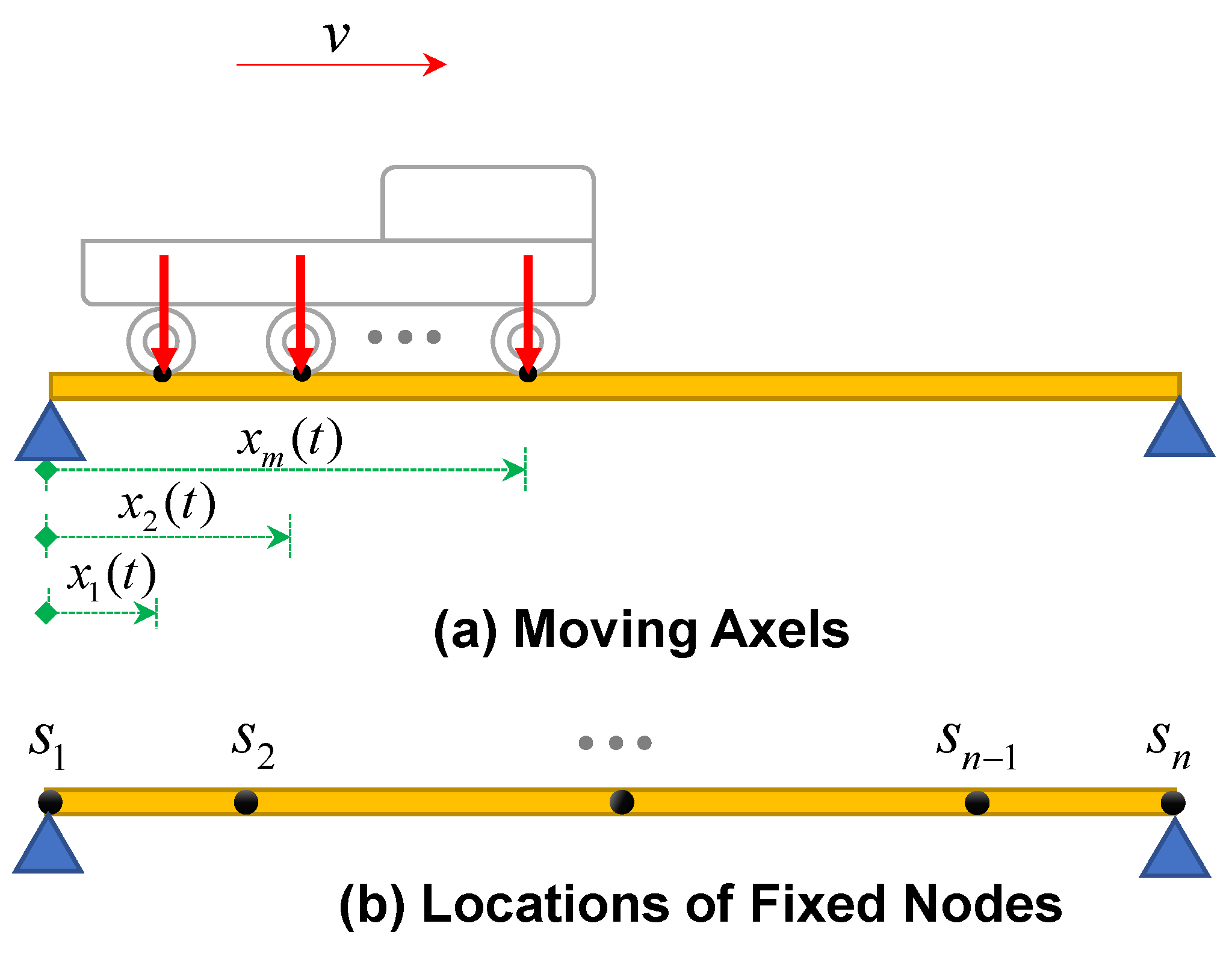
To predict the bridge response using the recorded acceleration responses from a crossing vehicle, the vehicle response needs to be spatially mapped onto some virtual fixed nodes on the bridge [
25]. These estimated responses can then be used to identify the dynamic characteristics and potential damages in the structure. However, due to the interpolation of the adjacent crossing axles (moving sensors), theoretical inverse problem solutions can only determine a limited part of the response signal for each fixed node on the bridge. This interpolation results in a sparse response matrix, where each row corresponds to the response of a particular fixed node and each column corresponds to the response vector of the fixed nodes in a time stamp. This matrix contains numerous missing values (invalid regions) that require advanced statistical, mathematical, or machine learning techniques to predict or complete the response signals for the virtual fixed nodes [
25,
26].
A few previous studies have utilized vehicle response data to identify bridge mode shapes using the sparse response data from bridges. While some of these methods have attempted to address the issue of missing values in the bridge response matrix through soft-imputing techniques [
26], short time frequency domain decomposition [
10], alternating least squares technique, and principal component analysis [
11], these approaches often rely on engineering judgment, involve time-consuming constrained optimization processes, and require manual parameter settings. Although these limited research works have made significant contributions to drive-by modal identification, there is a need for an innovative and automated framework to overcome these limitations.
This research work presents a novel technique for identifying the modal characteristics of bridges using only accelerometer sensors mounted on vehicles passing over them. The proposed framework consists of two stages. In the first stage, an inverse problem solution approach is employed to determine the acceleration and displacement response of virtual fixed nodes on the bridge. This is achieved by using the acceleration response of the vehicle axles as input, utilizing conventional linear interpolation functions to predict the bridge displacement responses, and introducing a novel cubic spline shape function to predict the acceleration response of the assumed fixed nodes on the bridge. However, the inverse problem solution approach yields response signals with missing parts, necessitating prediction. To address this issue, a new automated moving-window time series model based on auto-regressive exogenous (ARX) techniques is proposed in this paper. In the second stage, a novel approach combines the results of singular value decomposition (SVD) on the predicted displacement responses and frequency domain decomposition (FDD) on the predicted acceleration responses. This approach allows for the accurate identification of the first mode shape and higher mode shapes of the bridge, as well as the determination of natural frequencies. The main novelties of this research lie in the utilization of a cubic spline shape function within the inverse problem solution stage to predict the acceleration response of the fixed nodes and the application of moving-window time series models to complete the predicted incomplete signals obtained from the inverse problem solution procedure. Moreover, the method distinguishes itself by identifying mode shapes of the bridge using both acceleration and displacement responses, thereby enhancing the accuracy of identification for both lower and higher modes. Numerical simulations are conducted to evaluate the effectiveness of the proposed framework, considering different levels of ambient noise, number of axles, and vehicle speed. The future implementation of the framework in smartphone sensing-based applications is also discussed.
This paper is structured as follows:
Section 1 provides the introduction and review of the literature.
Section 2 focuses on the background and the inverse problem solution procedure, specifically for estimating the preliminary response signals of the bridge.
Section 3 introduces the details of the proposed framework, which encompasses a two-stage approach for predicting the missing parts of the response signals of the virtual fixed nodes on the bridge, as well as identifying the mode shapes and natural frequencies of the bridge. In
Section 4, numerical analyses are conducted to evaluate the performance of the proposed method. The results of the analyses are presented and discussed in
Section 5, where the characteristics and limitations of the proposed method are also examined. Finally,
Section 6 presents the conclusions of the study, along with recommendations for future research in this area.
3. Proposed Response Prediction and Modal Identification Methodology
The proposed framework from collecting the acceleration response of the crossing axles to identifying the modal characteristics of the bridge is summarized in
Figure 4. In this study, an inverse problem solution procedure is employed to estimate the initial displacement response signals of the bridge. Initially, a linear shape function is utilized for this purpose. However, based on numerical investigations, it has been demonstrated that incorporating a cubic spline shape function in the inverse solution procedure yields more precise results for bridge acceleration responses. The subsequent sub-section presents a detailed description of the proposed technique, which involves the use of a cubic spline interpolation function within the inverse problem solution procedure.
3.1. Continuous Cubic Spline as the Shape Function
A cubic spline is a piecewise polynomial in which the coefficients of each polynomial are fixed between joints [
29]. In this paper, an innovative approach to estimate the bridge nodal responses at the valid regions is proposed. The novelty of the proposed approach is utilizing cubic spline polynomials as the shape function for the displacement field in lieu of the conventional discontinuous linear ones (
Figure 5). Although a cubic spline interpolator is a continuous combination of some piecewise nonlinear cubic polynomials, it is shown that the linearity between the nodal responses and the response function will still be valid; the relation between the nodal responses and response field function can be written in the form of Equation (1).
It should be noted that natural spline is employed in this paper due to the fact that the first and last supports of bridges are generally roller or hinge type, which releases the moment reaction at the supports and results in zero curvature at those points (i.e.,
N″(
x = 0) and
N″(
x =
L) are considered zero).
where the matrix of coefficients
,
,
, and
are the size of
n by
n and to be calculated via the following equations and the row index,
j, can be valued from 1 to (
n − 1) [
29]:
In the previous equations, Δs is the distance between two adjacent virtual fixed nodes that can be assumed constant.
After the determination of N(x), the continuous response function of the bridge can be calculated by Equation (1).
3.2. Proposed Moving-Window ARX Model to Complete the Missing Parts of the Estimated Responses
As discussed in
Section 2, the classical method for solving the inverse problem can only estimate a small portion of the bridge displacement signal using drive-by data. In order to have the complete response for all the fixed nodes, a signal forecasting and completion approach is required.
In the present research, an innovative moving-window forecasting framework based on auto-regressive time series models with exogenous input (ARX) is introduced. The main motivation for this procedure is that the short valid part of the estimated response signal for a given fixed node can be trained by the corresponding parts of the responses of the adjacent nodes to forecast the missing response of the given node.
In other words, the proposed approach considers a unique ARX model for each of the fixed nodes. Therefore, (
n − 2) different ARX models can be established for the whole system. The proposed procedure can be utilized to forecast the missing parts of the signal in both backward and forward directions; however, it should be noted that, for training and predicting the missing parts in the backward direction, the reverse of the signals is used (see
Figure 6).
The ARX model structure is generally given by the following equation [
30]:
where
y(
t) and
u(
t) are the output and the input of the system, respectively;
, …,
and
, …,
are parameters of the model, which can be identified through the least-squares optimization approach;
e(
t) is a white-noise disturbance value.
The main reason for considering the ARX models is that the responses of two different fixed nodes located on the bridge can be decomposed to modal response components utilizing modal expansion principles for
nd modes [
31]:
In a general case, multiplying both sides of Equation (15) by the pseudoinverse of
Фs and substituting the resulting
Q(
t) in Equation (14) yields to Equation (17):
According to our numerical investigations, only the contribution of the adjacent nodes is high for the response prediction of the jth node. Therefore, we neglect the contributions of the other fixed nodes in Equation (17) and, by doing so, the pattern of the response can still be maintained.
Comparing Equation (17) with the general ARX model introduced in Equation (13), the time series model for the
jth node can be simplified as follows:
As obtained in Equation (18), the information on external force and vehicle characteristics in the proposed model is not required. The rationale behind considering a second-order ARX model is that using acceleration response in the time series model can give better accuracy.
By performing the proposed method for all the intermediate nodes, some parts of the bridge response signals can be completed according to
Figure 7. As can be seen from the figure, this approach is only able to complete the missing parts of the signal in which the input for the time series model can be provided, considering the missing gap between the two consecutive signals.
In order to complete the entire responses of the fixed nodes, the moving ARX algorithm will be applied through a straight-forward iterative procedure. The proposed signal completion framework is shown in
Figure 8 for the displacement response of an intermediate fixed node. It is important to highlight that the number of iterations needed depends on the quantity of moving axles and the number of virtual fixed nodes. For a model subjected to three-axle moving loads, a total of six iterations are required. As the number of axles increases, the number of iterations decreases due to a reduction in the valid regions. During each iteration of the algorithm, the predicted regions are combined with the initial valid regions, leading to an expansion of the valid regions within the response matrix. The iterative process continues until there are no remaining invalid regions in the response matrix.
3.3. Integrating Displacement and Acceleration Responses for Modal Identification
In this paper, a novel mode shape identification through the response of the moving wheels only is considered. To be more precise, both displacement and acceleration of the fixed nodes are first estimated with the aid of the proposed moving ARX method, then singular value decomposition (SVD) is applied on all of the nodal displacement responses to identify the first mode shape; however, for the higher modes and identification of natural frequencies, frequency domain decomposition (FDD) is utilized, considering the acceleration responses of the fixed nodes. This is based on the fact that combining displacement and acceleration responses in modal identification improves accuracy and reliability. Displacement responses are effective for identifying lower modes, while acceleration responses capture high-frequency components and higher modes more accurately [
32]. The mathematical relationship between accelerations and displacements reduces high-frequency components in dynamic displacements. This reduction is due to the fact that the integration operation acting as a low-pass filter and the accumulation of the area under the acceleration curve during integration [
33].
Since the SVD can extract the orthogonal vectors of an arbitrary matrix, it can be applied to the completed response matrix (
D) to determine
Фs:
where
U and
V are composed of the left and right singular vectors of matrix
D, respectively; they are orthogonal matrices.
Σ is a diagonal matrix containing singular values of
D.
By comparing the right side of Equations (15) and (19), identification of the mode shape can be performed with high accuracy [
25]:
We observed that SVD can identify the first mode shapes with high accuracy if applied on the displacement response matrix of the bridge.
As mentioned earlier, in order to identify the mode shapes through the acceleration response matrix of the bridge, the FDD method is employed [
34]. The basis of FDD is presented in the following paragraph.
From statistics, the correlation matrix between the response of the fixed nodes can be constructed using Equation (21):
Considering modal expansion and substituting Equation (15) in Equation (21) gives:
Then, taking Fourier transform from both sides of the latter equation produces the matrix containing cross/auto power spectrums of the response signals:
As can be understood from Equations (23) and (24), the SVD of matrix should be calculated for each frequency, ωi, in which the matrix of singular values (Σi) is a diagonal matrix containing modal FRFs and each column of the matrix of singular vectors (Ui and Vi) represents the mode shapes corresponding to the given frequency ωi.
4. Results
4.1. Model Setup
To evaluate the effectiveness of the proposed framework, a comprehensive numerical analysis is conducted on a single-span simply supported bridge using the finite element software package, ABAQUS. The bridge under consideration has a span length of 40 m and a rectangular cross-section with dimensions of 3 m wide and 1.5 m high. The material properties of the bridge are assigned based on concrete, with a density of 2400 kg/m3 and an elastic modulus of 27.5 GPa.
In the numerical model, the bridge is subjected to the loading of a three-axle moving vehicle. The distance between the axles is set to 2.5 m, as shown in
Figure 1. The natural frequencies of the bridge model are determined to be 1.44 Hz, 5.76 Hz, and 12.95 Hz for the first three modes, respectively.
A constant speed of 60 km/h is assigned to all the moving axles. The analysis is performed using a linear implicit dynamic analysis approach, considering the contacts between the moving axles and the bridge. The simulation is terminated when the foremost moving axle reaches the right end of the bridge.
For data acquisition, the accelerometers mounted on the moving vehicle have a constant sampling frequency of 200 Hz. Although a total of nine virtual fixed nodes are defined on the bridge, for the purpose of verification and comparison, only three specific fixed nodes located at ¼, ½, and ¾ of the span are selected to verify the displacement and acceleration responses.
Further details regarding the numerical model can be found in the previous work of the authors [
26]. The established numerical setup provides a realistic representation of a bridge structure and allows for the comprehensive evaluation of the proposed framework’s performance.
4.2. Interpretation of Results
As explained in
Section 2, by utilizing the measured acceleration of the moving axles in Equation (5), the valid part of the acceleration response signal of the fixed nodes on the bridge can be estimated. Similarly, to determine the displacement response signal, it is enough to double integrate the measured acceleration signals of the axles and put them in Equation (4).
In order to evaluate the proposed framework, the exact response of the fixed nodes on the bridge will be used directly from the numerical model. Although the acceleration and displacement responses of all nine fixed nodes can be determined using the proposed method, only the results from the linear and spline shape functions of three validation nodes are shown in
Figure 9 and
Figure 10.
The displacement and acceleration responses of the fixed nodes are determined using linear and spline shape functions, respectively, as outlined earlier.
Figure 9 shows that the cubic spline shape function proposed in this study provides more accurate acceleration response estimates of the fixed nodes in the valid regions compared with the conventional linear approach. On the other hand, the linear shape function provides more precise displacement response estimates compared with the cubic spline shape function (
Figure 10).
The difference observed between the linear and spline shape functions, regarding their impact on displacement response estimates, can be attributed to multiple factors. Firstly, the inherent characteristics of the displacement response itself play a significant role. Displacement responses primarily consist of low-frequency components that reflect the overall steady-state behavior of the system. The linear shape function, with its linear interpolation, aligns well with this low-frequency behavior, resulting in more precise displacement estimates.
Secondly, acceleration responses exhibit more complex dynamics and transient behaviors, often characterized by high-frequency oscillations. The cubic spline shape function, which incorporates higher-order interpolation, is better equipped to capture these intricate features, leading to more accurate estimates in the acceleration domain.
In summary, the choice between the linear and the spline shape functions depends on the specific nature of the response being analyzed. The linear shape function excels in capturing low-frequency displacement components, while the cubic spline shape function is advantageous for accurately representing the complex dynamics and high-frequency oscillations present in acceleration responses.
Hence, both responses of the fixed nodes are utilized in the proposed modal identification method. It is worth noting that higher accuracy of the determined responses in the valid regions results in higher accuracy of the predicted whole signals from the proposed moving time series model, based on the authors’ numerical observations.
The predicted displacement and acceleration responses of the bridge at the verification points, using only the measured acceleration of the moving axles and their relative amplitude errors, are presented in
Figure 11 and
Figure 12, respectively. The relative error of the predicted responses outside the valid regions is high in the case of a three-axle vehicle. However, as shown in the following sections, using more moving axles reduces these errors and, for all models, the mode shape identification accuracy is very high.
It is well known that the identification of lower modes of structures is easier using displacement responses, while higher modes can be identified using acceleration responses with higher accuracy [
33]. Accordingly, a hybrid mode shape identification framework is proposed, where SVD is applied to the predicted displacement responses of the fixed nodes (based on the linear shape function) to identify the first mode shape. On the other hand, the FDD technique is employed to identify the higher modes and natural frequencies by analyzing the acceleration responses (based on the cubic spline shape function) of the fixed nodes.
The results of the identified mode shapes and natural frequencies are presented in
Figure 13 and
Table 2, respectively. It is worth noting that the identified natural frequencies are based on the completed acceleration responses and considering the plot of the first singular value obtained from FDD.


